Towards optimal nonlinearities for sparse recovery using higher-order statistics

Abstract

We consider machine learning techniques to develop low-latency approximate solutions for a class of inverse problems. More precisely, we use a probabilistic approach to the problem of recovering sparse stochastic signals that are members of the $\ell_{p}$-balls. In this context, we analyze the Bayesian mean-square-error (MSE) for two types of estimators: (i) a linear estimator and (ii) a structured estimator composed of a linear operator followed by a Cartesian product of univariate nonlinear mappings. By construction, the complexity of the proposed nonlinear estimator is comparable to that of its linear counterpart since the nonlinear mapping can be implemented efficiently in hardware by means of look-up tables (LUTs). The proposed structure lends itself to neural networks and iterative shrinkage/thresholding-type algorithms restricted to a single iteration (e.g. due to imposed hardware or latency constraints). By resorting to an alternating minimization technique, we obtain a sequence of optimized linear operators and nonlinear mappings that converge in the MSE objective. The result is attractive for real-time applications where general iterative and convex optimization methods are infeasible.

Index Terms—  Probabilistic geometry, $\ell_{p}$-balls, compressive sensing, nonlinear estimation, Bayesian MMSE

1 Introduction

Precise error estimates and phase transitions play a crucial role in the analysis of compressed sensing recovery algorithms, where the objective is to recover an unknown $N$-dimensional real-valued vector signal $\bm{x}\in\mathbb{R}^{N}$ from a measurement vector $\bm{y}\in\mathbb{R}^{M}$ given by [1]

$${y}_{m} =\langle\bm{a}_{m},\bm{x}\rangle,\quad\forall m\in\{1,\ldots,M\},\ M<N.$$ (1)

Here and hereafter, $\langle\bm\cdot,\cdot\rangle:\mathbb{R}^{N}\times\mathbb{R}^{N}\to\mathbb{R}$ denotes the inner product in the Euclidean space $\mathbb{R}^{N}$, while the matrix $\bm{A}:=[\bm{a}_{1},\ldots,\bm{a}_{M}]^{T}\in\mathbb{R}^{M\times N}$ is a dimensionality reducing linear map that may be given or designed depending on the particular application. Motivated by the seminal work [1], we study a probabilistic approach to the above recovery problem, with the goal of assessing and optimizing the expected performance for a certain class of nonlinear estimators that can be implemented efficiently in hardware. In contrast to [1], we assume that the measurement map $\bm{A}$ is fixed and the randomness originates from a stochastic model of the estimand $\bm{x}$. It is therefore evident that the performance of any estimator (resp. recovery algorithm) will be tightly coupled to the statistical properties of the inner products in (1) with the sought sparse random vector $\bs{x}$. Among a myriad of models that have been proposed to analyze sparse/compressible signals at different layers of abstraction, the set of $k$-sparse signals $\Sigma_{k}:=\{\bm{x}:\lVert\bm{x}\rVert_{0}\leq k\}$, $k<N$, is frequent choice in the field of approximation theory (see e.g. [2]). The set $\Sigma_{k}$ is however of Lebesgue measure zero in $\mathbb{R}^{N}$, which makes the treatment within a unified probabilistic framework difficult. To overcome this limitation, we study the recovery of sparse stochastic signals from generalized unit balls $\mathcal{B}{p}$ that are equipped with the desired sparsity inducing structure for $\bm{p}<2\cdot\mathbb{1}$ and are closely related to the set $\Sigma_{k}$ [2] (see the definition of $\mathcal{B}{p}$ in Lemma 1 and Fig. 1 for an illustration). In this probabilistic $\mathcal{B}{p}$-model, the characteristic vector $\bm{p}$ adjusts the energy concentration in subsets of largest entries (in magnitude), i.e., the sparsity of realizations $\bm{x}$. In practice, we may use techniques from parametric density estimation to obtain estimates of the sparsity level in terms of $\bm{p}$ given some dataset. A review of selected existing and new results is provided in Sec. 2.

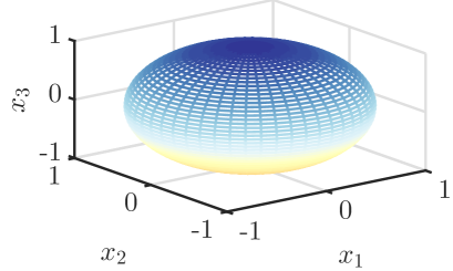
(a) $p=2$.

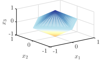
(b) $p=1$

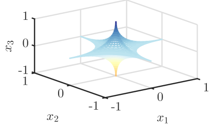
(c) $p=0.5$.

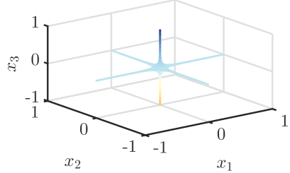
(d) $p=0.25$

Fig. 1: $\mathcal{B}{p}$ for various values of $\bm{p}=p\cdot\mathbb{1}$.

To simplify the subsequent exposition, we study the case of a uniform distribution on $\mathcal{B}{p}$, and note that more general (generalized-radial) distributions are subject to future works. Therefore, in all that follows, the probability distribution $p{x}(\bm{x})$ is assumed to be

$$p{x}(\bm{x})=\frac{1}{\mathrm{vol}(\mathcal{B}{p})}\mathds{1}_{\mathcal{B}{p}}(\bm{x}).$$ (2)

For brevity, we use $\bs{x}\sim\mathcal{U}(\mathcal{B}_{p})$ to refer to the random variable $\bs{x}$ drawn according to (2). Owing to the lack of space, we omit an in-depth discussion of stochastic models and refer an interested reader to the overview article on compressible distributions in [3] as well as the works on various sparse Lévy processes in [4]. Given the measurement model (1), we derive the Bayesian mean-squared-error (MSE) for a structured nonlinear estimator composed of a linear operator followed by a Cartesian product of univariate nonlinear mappings. For a recursive structure, a computationally much simpler approach can be found in [5] using a stochastic gradient method. While this amounts to a better scalability w.r.t. the problem dimension, the algorithm may converge slowly, or not at all, and missing error estimates may restrict its applicability. For the case of a polynomial mapping in canonical form, we analyze an alternating optimization approach that is guaranteed to converge w.r.t. the MSE objective. The latter is shown be to computable in closed-form as a function of higher-order inner product statistics.

Remark 1 (Bayesian vs. classical MMSE estimation).

We highlight that the present paper targets the Bayesian MSE as opposed to classical MSE estimation. In the Bayesian setting, an optimal estimator in the sense of an average performance criterion is obtained under the assumption of a prior pdf of the estimand. As such, the optimal Bayesian estimator for the MSE criterion is given by the conditional mean, which is in general hard to obtain and is approximated in a hardware-efficient manner in this work. On the other hand, in classical MSE estimation, a certain realization of sparse vector $\bm{x}$ is chosen and an optimal estimator for the particular given case is sought. For the latter case, the optimal estimator is often not realizable due to its dependence on the particular realization $\bm{x}$ (see also [6][Ch. 10] for additional illustrative examples).

1.1 Notation

Scalar, vector and matrix random variables are denoted by lowercase, bold lowercase and bold uppercase sans-serif letters $\ms{x}$, $\bs{x}$, $\bs{X}$, while the corresponding realizations by serif letters $x$, $\bm{x}$, $\bm{X}$. The sets of reals, nonnegative reals, positive reals, nonnegative integers and natural numbers are designated by $\mathbb{R}$, $\mathbb{R}_{+}$, $\mathbb{R}_{++}$, $\mathbb{N}_{0}$ and $\mathbb{N}$. We use $\mathbb{0}$, $\mathbb{1}$ and $\bm{I}$ to denote the vectors of all zeros, all ones and the identity matrix, where the size will be clear from the context. $\mathrm{tr}\{\cdot\}$, $\mathrm{diag}(\bm{u})$, $(\cdot)^{\odot d}$ and $\mathds{1}_{\mathcal{X}}:\bm{x}\to\{0,1\}$ denote the trace of a matrix, the diagonal matrix with elements of $\bm{u}$ on the diagonal, the hadamard (i.e. entry-wise) power and the indicator function defined as $\mathds{1}_{\mathcal{X}}(\bm{x})=1$ if $\bm{x}\in\mathcal{X}$ and $0$ otherwise. $\mathcal{U}(\mathcal{X})$ is used to denote the uniform distribution over the set $\mathcal{X}$, $\mathbb{E}\left[\cdot\right]$ is the expectation operator and $\mathcal{B}{p}$ is the generalized unit ball defined in Lemma 1.

2 A primer for signals from $\mathcal{B}{p}$

Given the probability distribution in (2) the first question is if $\mathrm{vol}(\mathcal{B}_{p})$ can be obtained in closed form for general vectors $\bm{p}$ without using multivariate approximation techniques (e.g. cubature formulae) that are known to suffer from the so-called curse of dimensionality. It is interesting to note that an affirmative answer to this question can be traced back to works by Dirichlet on the Laplace transform [7] as was noted in [8] and appeared in different works from control theory to Banach space geometry (see [9, 10]). The respective result is restated in the following Lemma.

Lemma 1 (Volume of generalized unit balls $\mathcal{B}{p}$).

Let $\bm{p}\in\mathbb{R}_{++}^{N}$, $\mathcal{B}{p}$ be given by $\mathcal{B}{p}:=\{\bm{x}:\sum_{n=1}^{N}\lvert x_{n}\rvert^{p_{n}}\leq 1\}\subset\mathbb{R}^{N}$ and

$$\Gamma(z):=\int_{0}^{\infty}t^{z-1}\exp(-t)\,dt$$ (3)

denote the Gamma function (see [11] for a review of mathematical properties). Then, it holds that

$$\mathrm{vol}(\mathcal{B}{p})=\frac{2^{N}}{\prod_{n=1}^{N}p_{n}}\frac{\prod_{n=1}^{N}\Gamma\left(\frac{1}{p_{n}}\right)}{\Gamma\left(1+\sum_{n=1}^{N}\frac{1}{p_{n}}\right)}.$$ (4)

Proof.

The proof can be found e.g. in [8]. ∎

As an extension of Lemma 1, we obtain the following result for the integral as well as expectation of a monomial over $\mathcal{B}{p}$ w.r.t. to the measure (2), which forms the basis for the subsequent analysis.

Lemma 2 (Expectation of monomials over $\mathcal{B}{p}$).

Let $\bm{x}^{\boldsymbol{\alpha}}$ denote the monomial ${x}_{1}^{\alpha_{1}}\cdots{x}_{N}^{\alpha_{N}}$ with $\bm{x}\in\mathbb{R}^{N}$ and $\boldsymbol{\alpha}\in\mathbb{N}_{0}^{N}$, $\bs{x}\sim\mathcal{U}(\mathcal{B}{p})$, and $2\mathbb{N}_{0}:=\{2\beta:\beta\in\mathbb{N}_{0}\}$ be the set of nonnegative even integers. Then, we have

$$\int_{\mathcal{B}{p}}\bm{x}^{\boldsymbol{\alpha}}\ d\bm{x} =\begin{cases}\frac{2^{N}}{\prod_{n=1}^{N}p_{n}}\frac{\prod_{n=1}^{N}\Gamma\left(\frac{\alpha_{n}+1}{p_{n}}\right)}{\Gamma\left(1+\sum_{n=1}^{N}\frac{\alpha_{n}+1}{p_{n}}\right)}&\text{for }\boldsymbol{\alpha}\in 2\mathbb{N}_{0}^{N}\\ 0&\text{otherwise},\end{cases}$$

and

$$\mathbb{E}{x}\left[\bs{x}^{\boldsymbol{\alpha}}\right]=\frac{1}{\mathrm{vol}(\mathcal{B}{p})}\int_{\mathcal{B}{p}}\bm{x}^{\boldsymbol{\alpha}}\ d\bm{x}.$$ (5)

Proof.

The proof is deferred to Appendix A. ∎

Of course, $\mathrm{vol}(\mathcal{B}{p})$ can be obtained similarly as a special case of Lemma 2 using $\boldsymbol{\alpha}=\mathbb{0}$. In the subsequent analysis, we also need to evaluate higher-order statistics of an inner product of $\bs{x}$ and some given $\bm{u}\in\mathbb{R}^{N}$, which is formalized in the following Lemma.

Lemma 3 (Higher-order inner-product statistics).

Let $\bs{x}\sim\mathcal{U}(\mathcal{B}{p})$, $\boldsymbol{\alpha}\in\mathbb{N}_{0}^{N}$, $d\in\mathbb{N}_{0}$ and $\bm{u}\in\mathbb{R}^{N}$ be a given vector. Then, using

$${d\choose\boldsymbol{\alpha}}=\frac{d!}{\prod_{n=1}^{N}(\alpha_{n}!)},$$ (6)

we obtain

$$\mathbb{E}{x}\left[\langle\bm{u},\bs{x}\rangle^{d}\right]=\sum\nolimits_{\lVert\boldsymbol{\alpha}\rVert_{1}=d}{d\choose\boldsymbol{\alpha}}\bm{u}^{\boldsymbol{\alpha}}\mathbb{E}{x}\left[\bs{x}^{\boldsymbol{\alpha}}\right],$$ (7)

$$\mathbb{E}{x}\left[\ms{x}_{i}\langle\bm{u},\bs{x}\rangle^{d}\right]=\sum\nolimits_{\lVert\boldsymbol{\alpha}\rVert_{1}=d}{d\choose\boldsymbol{\alpha}}\bm{u}^{\boldsymbol{\alpha}}\mathbb{E}{x}\left[\bs{x}^{\boldsymbol{\alpha}+\bm{e}_{i}}\right],$$ (8)

$$\mathbb{E}{x}\left[\ms{x}_{i}\ms{x}_{j}\langle\bm{u},\bs{x}\rangle^{d}\right]=\sum\nolimits_{\lVert\boldsymbol{\alpha}\rVert_{1}=d}{d\choose\boldsymbol{\alpha}}\bm{u}^{\boldsymbol{\alpha}}\mathbb{E}{x}\left[\bs{x}^{\boldsymbol{\alpha}+\bm{e}_{i}+\bm{e}_{j}}\right],$$ (9)

where $\bm{e}_{i}$ denotes the $i$-th standard Euclidean basis vector in $\mathbb{R}^{N}$.

Proof.

The Lemma follows from an application of the multinomial formula

$$\left(u_{1}\ms{x}_{1}+u_{2}\ms{x}_{2}+\ldots+u_{N}\ms{x}_{N}\right)^{d}=\sum\nolimits_{\lVert\boldsymbol{\alpha}\rVert_{1}=d}{d\choose\boldsymbol{\alpha}}\bm{u}^{\boldsymbol{\alpha}}\bs{x}^{\boldsymbol{\alpha}}$$ (10)

together with the linearity of the expectation operator. ∎

In Fig. 2 we illustrate similarities and differences of various sparse processes that can be encountered in literature. The respective probability density functions are given in Tab. 1. For a practical algorithm and implementation to generate signals from $\mathcal{B}{p}$ we refer the interested reader to [9], which was also used for the Monte-Carlo simulations in Sec. 5.

Model	$p{x}(\bm{x})$
Gaussian	$\frac{1}{(2\pi\sigma^{2})^{\frac{N}{2}}}e^{-\frac{\lVert\bm{x}\rVert_{2}^{2}}{\sigma^{2}}}$
Laplace	$\left(\frac{\lambda}{2}\right)^{N}e^{-\lambda\lVert\bm{x}\rVert_{1}}$
Compound Poisson,	$\prod_{n=1}^{N}\Big{(}e^{-\lambda}\delta(x_{n})+$
Gaussian amplitude	$+(1-e^{-\lambda})\frac{1}{\sqrt{2\pi\sigma^{2}}}\exp\left(\frac{-x_{n}^{2}}{2\sigma^{2}}\right)\Big{)}$
uniform $\mathcal{B}{p}$	$\frac{1}{\mathrm{vol}(\mathcal{B}{p})}\mathds{1}_{\mathcal{B}{p}}(\bm{x})$

Table 1: PDFs of various (sparse) processes.

3 Bayesian estimators for signals from $\mathcal{B}{p}$

3.1 MAP estimation

We start this section with a brief review of general Bayesian estimators following a standard textbook in the field [6].

Definition 1 (MAP estimator).

Let $\bm{y}$ be defined by (1) and $p{x}(\bm{x})$ be given by (2). A MAP estimate

$$\hat{\bm x}_{\mathrm{map}}\in{\mathrm{argmax}{x}}\ p_{\bs{y}|\bs{x}}(\bm{y}|\bm{x})p{x}(\bm{x})$$ (11)

is given by

$$\hat{\bm x}_{\mathrm{map}}\in{\mathrm{argmax}{x}}\ \delta(\bm{y}-\bm{A}\bm{x})p_{\bs{x}}(\bm{x}).$$ (12)

Here, $\delta(\bm{z})$ denotes the idealized dirac-delta point mass at $\bm{z}=\mathbb{0}$. We note that (12) can be equivalently written as

$$\hat{\bm x}_{\mathrm{map}}\in\left(\bm{x}_{0}+\mathrm{null}(\bm{A})\right)\cap\mathcal{B}{p},$$ (13)

where $\bm{x}_{0}$ is an arbitrary point satisfying $\bm{y}=\bm{A}\bm{x}_{0}$.

The MAP estimator provides an excellent estimation performance, but it usually amounts to solving a costly optimization problem rendering it infeasible for most real-time applications. Some relevant examples of such applications in the field of communications include sparse channel estimation [12] and sparse multiuser detection [13], where the interest is in the development of dedicated chips based on integrated circuit (IC) architectures that exploit pipelining as well as parallelism. In such settings, even a seemingly simple matrix-inverse is usually avoided as it scales cubic in the number of inputs [12].

3.2 Linear Bayesian MMSE estimation

We proceed with low-complexity linear Bayesian MMSE (LMMSE) estimators that, whilst being inferior to the MAP in terms of estimation performance, may be easily implemented and often offer acceptable performance guarantees.

Definition 2 (Linear Bayesian MMSE).

Let $\bm{y}$ and $p{x}(\bm{x})$ be given by (1) and (2). The linear Bayesian MMSE estimator $\bm{W}_{\mathrm{lmmse}}$ is the solution to

$$\bm{W}_{\mathrm{lmmse}}\in\underset{\bm{W}\in\mathbb{R}^{N\times M}}{\mathrm{argmin}}\ \mathbb{E}{x}\left[\lVert\bs{x}-\bm{W}\bm{A}\bs{x}\rVert_{2}^{2}\right],$$ (14)

where the expectation is taken w.r.t. $\bs{x}\sim\mathcal{U}(\mathcal{B}{p})$.

Theorem 1 (Linear Bayesian MMSE).

Let $\bm{y}$ be given by (1) and $p{x}(\bm{x})$ by (2). Assuming that the inverse exists, the optimal linear estimator according to Def. 2 can be obtained by

$$\bm{W}_{\mathrm{lmmse}}=\bm{C}_{\bs{x}}\bm{A}^{T}\left(\bm{A}\bm{C}_{\bs{x}}\bm{A}^{T}\right)^{-1}$$ (15)

with $\bm{C}_{\bs{x}}:=\mathbb{E}\left[\bs{x}\bs{x}^{T}\right]$ given by

$$[\bm{C}_{\bs{x}}]_{i,j}:=\mathbb{E}{x}\left[\bs{x}^{\bm{e}_{i}+\bm{e}_{j}}\right].$$ (16)

Proof.

The proof is a standard results in Bayesian MMSE estimation (see e.g. [6, p. 364]). ∎

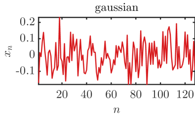
(a) Gaussian distribution (not sparse) with $\mu=0$, $\sigma=1$.

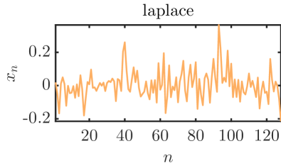
(b) Laplace distribution with $\lambda=5$.

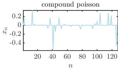
(c) Compount poisson distribution with $\lambda=0.25$, $\mu=0$, $\sigma=1$.

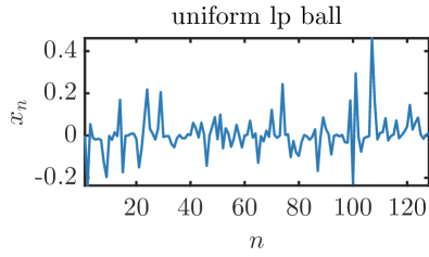
(d) Uniform $\mathcal{B}{p}$ with $\bm{p}=0.33\cdot\mathbb{1}$.

Fig. 2: Realizations of various (sparse) processes in $\mathbb{R}^{128}$. Signals are normalized to unit $\ell_{2}$-norm.

The corresponding Bayesian MSE is given by

$$\varepsilon_{\mathrm{lmse}}(\bm{W})= \mathbb{E}{x}\left[\lVert\bs{x}-\bm{W}\bm{A}\bs{x}\rVert_{2}^{2}\right]=\mathrm{tr}\left\{\bm{C}_{\bs{x}}\right\}-2\mathrm{tr}\left\{\bm{W}\bm{A}\bm{C}_{\bs{x}}\right\}$$

$$+\mathrm{tr}\left\{\bm{A}^{T}\bm{W}^{T}\bm{W}\bm{A}\bm{C}_{\bs{x}}\right\}.$$ (17)

3.3 Structured nonlinear estimation

An increasingly popular technique for recovering sparse signals consists in using a linear mapping followed by a Cartesian product of univariate nonlinearities (e.g. classical or learned iterative shrinkage-thresholding algorithms [14],[5]) in an alternating fashion. As a conceptual analogue, we propose a nonlinear Bayesian MMSE estimator using a similar structural assumption.

Proposition 1 (Structured nonlinear MMSE estimator).

Let $\mathcal{T}:=\mathcal{T}_{1}\times\ldots\times\mathcal{T}_{N}:\mathbb{R}\times\ldots\times\mathbb{R}\mapsto\mathbb{R}\times\ldots\times\mathbb{R}$ be a Cartesian product of univariate nonlinear mappings and define the sructured Bayesian MMSE (SMMSE) estimator to be of the form

$$\hat{\bm x}=\mathcal{T}\left(\bm{W}\bm{y}\right)=\mathcal{T}\left(\bm{W}\bm{A}\bm{x}\right),$$ (18)

where for ease of practical realization we further impose equality among the nonlinear mappings, i.e., $\mathcal{T}_{1}=\ldots=\mathcal{T}_{N}$.

An illustration of the SMMSE estimators’ structure is shown in Fig. 3.

\psfrag{s}[bc][bc]{$\bm{W}$}\psfrag{y1}[bc][bc]{${y}_{1}$}\psfrag{yK}[bc][bc]{${y}_{M}$}\psfrag{x1}[bc][bc]{${x}_{1}$}\psfrag{xK}[bc][bc]{${x}_{N}$}\psfrag{t1}[bc][bc]{${\hat{x}}_{1}$}\psfrag{tK}[bc][bc]{${\hat{x}}_{N}$}\psfrag{A}[bc][bc]{$\bm{A}$}\psfrag{W}[bc][bc]{$\bm{W}$}\psfrag{T}[bc][bc]{$\mathcal{T}$}\includegraphics[width=411.93767pt]{nnet_2.eps}

Fig. 3: Structured nonlinear Bayesian MMSE estimator composed of a linear map $\bm{W}$ and a Cartesian product of univariate nonlinear maps $\mathcal{T}:=[\mathcal{T}_{1}\cdots\mathcal{T}_{N}]^{T}$.

In this paper, we analyze explicitly the canonical polynomial map

$$\mathcal{T}_{i}(t):=\sum\nolimits_{d=0}^{D}a_{d}t^{d}$$ (19)

resulting in an estimate

$$\hat{\bm x}=\sum\nolimits_{d=0}^{D}a_{d}\left(\bm{W}\bm{A}\bm{x}\right)^{\odot d}.$$ (20)

Accordingly, the corresponding Bayesian MSE is given by

$$\varepsilon_{\mathrm{smse}}(\bm{a},\bm{W}) =\mathbb{E}{x}\left[\lVert\bs{x}-\bs{\hat{x}}\rVert_{2}^{2}\right]$$

$$=\mathrm{tr}\left\{\bm{C}_{\bs{x}}\right\}-2\mathrm{tr}\left\{\bm{C}_{\bs{x}\bs{\hat{x}}}\right\}+\mathrm{tr}\left\{\bm{C}_{\bs{\hat{x}}}\right\},$$ (21)

where $\mathrm{tr}\left\{\bm{C}_{\bs{x}}\right\}$ follows from Th. 1. The two other terms are equal to

$$\mathrm{tr}\left\{\bm{C}_{\bs{x}\bs{\hat{x}}}\right\} =\mathrm{tr}\left\{\mathbb{E}{x}\left[\sum_{d=0}^{D}a_{d}\mathrm{diag}^{d}\left(\bm{W}\bm{A}\bs{x}\right)\mathrm{diag}(\bs{x})\right]\right\}$$ (22)

$$=\mathbb{E}{x}\left[\mathrm{diag}(\bs{x})\bm{V}\right]\bm{a}$$ (23)

$$\mathrm{tr}\left\{\bm{C}_{\bs{\hat{x}}}\right\} =\mathrm{tr}\left\{\mathbb{E}{x}\left[\sum_{i=0}^{D}\sum_{j=0}^{D}a_{i}a_{j}\mathrm{diag}^{i+j}\left(\bm{W}\bm{A}\bs{x}\right)\right]\right\}$$ (24)

$$=\bm{a}^{T}\mathbb{E}{x}\left[\bm{V}^{T}\bm{V}\right]\bm{a},$$ (25)

where we use the convention that $\mathrm{diag}^{0}(\bm{u})=\bm{I}$ and define the Vandermonde matrix $\bm{V}$ as

$$\bm{V}:=\left[\mathbb{1},(\bm{W}\bm{A}\bs{x})^{\odot 1},\ldots,(\bm{W}\bm{A}\bs{x})^{\odot D}\right].$$ (26)

To obtain (22)-(25) we define $\bm{U}=[\bm{u}_{1},\ldots,\bm{u}_{n}]^{T}:=\bm{W}\bm{A}$ and apply Lemma 3 to compute the required expectations entrywise:

$$\left\{\mathbb{E}{x}\left[\bs{x}^{T}\bm{V}\right]\right\}_{i,j}=\mathbb{E}{x}\left[\ms{x}_{i}\langle\bm{u}_{i},\bs{x}\rangle^{j-1}\right]$$ (27)

$$\qquad\qquad\ \forall\{i,j\}\in\{1,\ldots,N\}\times\{1,\ldots,D+1\},$$

$$\left\{\mathbb{E}{x}\left[\bm{V}^{T}\bm{V}\right]\right\}_{i,j}=\sum_{n=1}^{N}\mathbb{E}{x}\left[\langle\bm{u}_{n},\bs{x}\rangle^{i+j-2}\right]$$ (28)

$$\qquad\qquad\ \forall\{i,j\}\in\{1,\ldots,N\}^{2}.$$

4 Alternating minimization of the SMSE

The aim of this section is to derive an algorithmic solution to the minimization of the Bayesian SMSE (3.3), i.e., solving (approximately) the problem

$$\underset{\begin{subarray}{c}\bm{a}\in\mathbb{R}^{D+1}\\ \bm{W}\in\mathbb{R}^{N\times M}\end{subarray}}{\min}\ \varepsilon_{\mathrm{smse}}(\bm{a},\bm{W}).$$ (29)

The reader should note that for $\bm{a}:=\bm{e}_{2}\in\mathbb{R}^{D+1}$ the problem reduces to the LMMSE setting from Th. 1. As such, the LMMSE estimator is a particular instance of the SMMSE estimator, and therefore it yields an upper bound on the achievable MSE. On the other hand, the integrand (expectation) in (3.3) is nonnegative for every $\bm{x}\in\mathcal{B}{p}$. Hence, we can write

$$0\leq\underset{\begin{subarray}{c}\bm{a}\in\mathbb{R}^{D+1}\\ \bm{W}\in\mathbb{R}^{N\times M}\end{subarray}}{\min}\ \varepsilon_{\mathrm{smse}}(\bm{a},\bm{W})\leq\underset{\bm{W}\in\mathbb{R}^{N\times M}}{\min}\ \varepsilon_{\mathrm{lmse}}(\bm{W}).$$ (30)

A widely-used algorithm for optimization problems with block partitioned arguments is the alternating minimization algorithm (AMA) [16], which is also often referred to as block coordinate descent method [15], given in Alg. 1 for Problem (29).

Input: $\bm{W}_{\star}^{(0)}$, $\bm{a}_{\star}^{(0)}$

Output: $\bm{W}^{\star}$, $\bm{a}^{\star}$

for $k=0,1,\ldots$ do  $\displaystyle\bm{a}_{\star}^{(k+1)}$ $\displaystyle\in\ \underset{\bm{a}\in\mathbb{R}^{D+1}}{\mathrm{argmin}}\ \varepsilon_{\mathrm{smse}}(\bm{a},\bm{W}_{\star}^{(k)})$ (31a) $\displaystyle\bm{W}_{\star}^{(k+1)}$ $\displaystyle\in\ \underset{\bm{W}\in\mathbb{R}^{N\times N}}{\mathrm{argmin}}\ \varepsilon_{\mathrm{smse}}(\bm{a}_{\star}^{(k+1)},\bm{W})$ (31b) end

Algorithm 1 Alternating minimization algorithm.

The algorithm generates a non-increasing sequence of objective values since

$$\forall k\in\mathbb{N}_{0}:\ \varepsilon_{\mathrm{smse}}(\bm{a}_{\star}^{(k)},\bm{W}_{\star}^{(k)}) \geq\varepsilon_{\mathrm{smse}}(\bm{a}_{\star}^{(k+1)},\bm{W}_{\star}^{(k)})\geq$$ (32)

$$\geq\varepsilon_{\mathrm{smse}}(\bm{a}_{\star}^{(k+1)},\bm{W}_{\star}^{(k+1)}).$$ (33)

Due to the monotone convergence theorem a first consequence is that Alg. 1 converges w.r.t. the MSE objective, since by (30) the objective function is bounded from below. It was shown in [16] that in convex as well as non-convex settings the generated sequence of solutions $(\bm{a}_{\star}^{(k)},\bm{W}_{\star}^{(k)})$ converges to a critical point of problem (29) (provided that the generated sequence admits limit points and for each subproblem of Alg. 1 the minimum is uniquely attained). The latter non-convex setting indeed applies to Problem (29) as can be seen from the optimization variable $\bm{W}$ being the argument of a generally non-convex polynomial map.

We highlight that from a numerical viewpoint the aforementioned convergence to critical points may not be guaranteed (i.e. we may suffice ourselves with monotone convergence w.r.t. the MSE objective) since the assumption that optimal solutions to every subproblem (31b) of Alg. 1 can be computed is usually violated. For an accompanying numerical implementation of Alg. 1, we first note that if the matrix $\mathbb{E}{x}\big{[}\bm{V}^{T,(k)}\bm{V}^{(k)}\big{]}$ is positive-definite, then the first subproblem (31a) is strictly convex and admits a closed form solution by exploiting the first-order optimality condition

$$\frac{\partial}{\partial\bm{a}}\varepsilon :=\begin{bmatrix}\frac{\partial\varepsilon}{\partial a_{0}}&\cdots&\frac{\partial\varepsilon}{\partial a_{D}}\end{bmatrix}^{T}$$ (34)

$$=-2\mathbb{E}{x}\left[\bm{V}^{(k),T}\bs{x}\right]+2\mathbb{E}{x}\left[\bm{V}^{(k),T}\bm{V}^{(k)}\right]\bm{a}\stackrel{{\scriptstyle!}}{{=}}\mathbb{0}.$$ (35)

Using (26) for some given $\bm{W}^{(k)}$ we obtain a numerical solution

$$\bm{a}_{\diamond}^{(k+1)}:=\mathbb{E}{x}\left[\bm{V}^{T,(k)}\bm{V}^{(k)}\right]^{-1}\mathbb{E}{x}\left[\bm{V}^{T,(k)}\bs{x}\right].$$ (36)

For the generally non-convex subproblem (31b) we propose a numerical implementation based on a simple steepest-descent iteration to find a critical point $\bm{W}_{\diamond}^{(k)}$ as an approximation to the optimal solution $\bm{W}_{\star}^{(k)}$ using the following result for the partial derivative defined as

$$\frac{\partial}{\partial\bm{W}}\varepsilon:=\begin{bmatrix}\frac{\partial\varepsilon}{\partial{W}_{1,1}}&\cdots&\frac{\partial\varepsilon}{\partial W_{1,M}}\\ \vdots&\ddots&\vdots\\ \frac{\partial\varepsilon}{\partial{W}_{N,1}}&\cdots&\frac{\partial\varepsilon}{\partial{W}_{N,M}}\end{bmatrix}.$$ (37)

Proposition 2.

Let $\mathrm{tr}\left\{\bm{C}_{\bs{x}\bs{\hat{x}}}\right\}$ and $\mathrm{tr}\left\{\bm{C}_{\bs{\hat{x}}}\right\}$ be given by (22) and (24). Then, it holds that

$$\frac{\partial}{\partial\bm{W}}\mathrm{tr}\left\{\bm{C}_{\bs{x}\bs{\hat{x}}}\right\}=\mathbb{E}{x}\left[\sum\nolimits_{d=1}^{D}da_{d}\mathrm{diag}^{d-1}(\bm{W}\bm{A}\bs{x})\bs{x}\bs{x}^{T}\bm{A}\right]$$ (38)

and

$$\frac{\partial}{\partial\bm{W}}\mathrm{tr}\left\{\bm{C}_{\bs{\hat{x}}}\right\}=$$ (39)

$$=\mathbb{E}{x}\left[\sum_{k=0}^{D}\sum_{\begin{subarray}{c}l=0\\ [k,l]\neq\mathbb{0}\end{subarray}}^{D}(k+l)a_{k}a_{l}\mathrm{diag}^{k+l-1}(\bm{W}\bm{A}\bs{x})\mathbb{1}\bs{x}^{T}\bm{A}^{T}\right].$$

Proof.

The proof is deferred to Appendix B. ∎

To compute the expectations in Prop. 2 we use Lemma 3 and evaluate the matrix numerically to obtain

$$\left[\frac{\partial}{\partial\bm{W}}\mathrm{tr}\left\{\bm{C}_{\bs{x}\bs{\hat{x}}}\right\}\right]_{i,j}=\sum_{d=1}^{D}da_{d}\mathbb{E}{x}\left[\ms{x}_{i}\ms{x}_{j}\langle\bm{u}_{i},\bs{x}\rangle^{d-1}\right],$$ (40)

$$\left[\frac{\partial}{\partial\bm{W}}\mathrm{tr}\left\{\bm{C}_{\bs{\hat{x}}}\right\}\right]_{i,j}=\sum_{k=0}^{D}\sum_{\begin{subarray}{c}l=0\\ [k,l]\neq\mathbb{0}\end{subarray}}^{D}(k+l)a_{k}a_{l}\mathbb{E}{x}\left[\ms{x}_{j}\langle\bm{u}_{i},\bs{x}\rangle^{i+j-1}\right]$$

$\forall\{i,j\}\in\{1,\ldots,N\}^{2}$. A further description of the numerical implementation is provided in the following Section.

5 Numerical Results

To obtain the proposed structured Bayesian MMSE estimator, we solve the optimization problem (31) using the update (36) for (31a) and a reference implementation of the steepest-descent algorithm with Armijo line-search [17] using the gradients (38), (39) for (31b). We evaluate the normalized MSE defined as

$$\mathrm{NMSE}:=\varepsilon(\bm{a}_{\diamond},\bm{W}_{\diamond})/\mathrm{tr}(\bm{C}{x})$$ (41)

for a set of structurally different sensing matrices $\bm{A}\in\mathbb{R}^{3\times 6}$ given as

1. an equiangular tight frame (i.e. $\bm{A}_{1}:=[\bm{a}_{1},\ldots,\bm{a}_{6}]$ s.t. $\lVert\bm{a}_{i}\rVert_{2}=1\ \forall i$ and $\lvert\langle\bm{a}_{i},\bm{a}_{j}\rangle\rvert={\sqrt{N-M}}/{\sqrt{M(N-1)}}$ $\forall i\neq j$),

2. a subsampled orthogonal matrix $\bm{A}_{2}$ (with $\bm{A}_{2}\bm{A}_{2}^{T}=\bm{I}$), and

3. a random matrix generated by drawing i.i.d. Gaussian entries followed by a normalization of rows.

The remaining parameters are $\bm{p}:=p\cdot\mathbb{1}$ with $p\in[0.4,2]$ and the polynomial map is set to degree $D=9$. As initial values we use $\bm{a}_{\diamond}^{(0)}=\mathbb{0}$ and a scaled Moore-Penrose pseudo-inverse $\bm{W}_{\diamond}^{(0)}=c\bm{A}^{\dagger}$, with scaling set to $c=10$ to stabilize the polynomial map, that were found experimentally. The results in terms of the $\mathrm{NMSE}$ are shown in Fig. 4 and in terms of the optimal nonlinearities of the polynomial map for $\bm{A}_{1}$ in Fig. 5. For comparison, we also show the results for $\ell_{1}$-minimization (i.e. $\bm{\hat{x}}\in\mathrm{argmin}_{\bm{A}\bm{x}=\bm{y}}\bm{x}$) for $p\leq 1$ which were obtained using CVX [18]. We note that for this case $\ell_{1}$-minimization yields an interior point in the convex-hull $\mathcal{B}_{\mathbb{1}}\supseteq\mathcal{B}_{\bm{p}\leq\mathbb{1}}$ which should be a good approximation of the MAP estimate (12). Due to the high complexity of obtaining the optimal numerical parameters $(\bm{a}_{\diamond},\bm{W}_{\diamond})$ of the structured Bayesian MMSE estimator using the described numerical approximation of Alg. 1, we limit our analysis to the low-dimensional setting and defer the high-dimensional analysis to a future study using e.g. faster approximate methods. We note, that the upper bound $0.5$ of the $\mathrm{NMSE}$ results from the compression factor $M/N$. It is interesting to see that the nonlinear Bayesian MMSE estimator in conjunction with the equiangular tight frame $\bm{A}_{1}$ resulted in the highest performance gains, with an approximate performance increase of (i) $20\,\%$, (ii) $15\,\%$ and (iii) $13\,\%$ over (i) the linear estimator (independent of the mapping $\bm{A}$), (ii) the subsampled orthogonal matrix and (iii) the normalized i.i.d. matrix. The optimization to obtain the SMMSE estimator for the predetermined set of sensing matrices and characteristic vectors was performed offline using an Amazon AWS c4.8xlarge instance and $36$ parallel threads. In terms of complexity, the estimation of $\bm{\hat{x}}$ given $\bm{A}_{i\in\{1,2,3\}}\bm{x}$ by the SMMSE estimator was observed to be more then a thousand-fold faster than $\ell_{1}$-minimization on a laptop with i7-2.9 GHz processor.

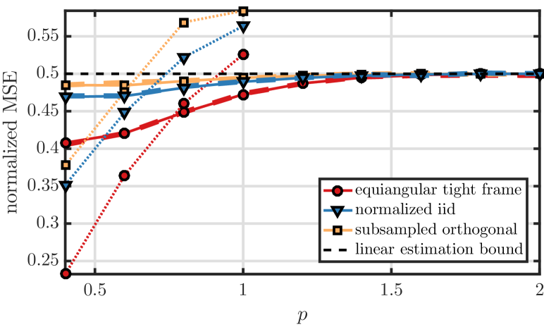
Fig. 4: Normalized MSE for the proposed estimator and varying matrices $\bm{A}$. Analytical results from (3.2) are shown in solid, Monte-Carlo results in dashed and results for $\ell_{1}$-minimization in dotted linestyle.

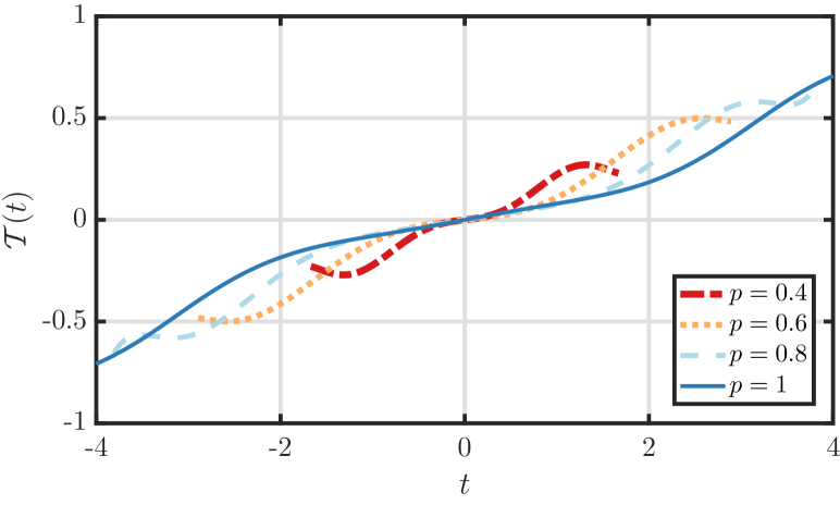
Fig. 5: Optimal nonlinearities $\mathcal{T}$ for equiangular tight frame $\bm{A}_{1}$ and varying values of $p$ plotted over $\pm\mathrm{sup}_{\bm{x}\in\mathcal{B}{p}}\lVert\bm{W}_{\diamond}\bm{A}_{1}\bm{x}\rVert_{\infty}$.

6 Conclusion

In this paper we proposed a structured nonlinear Bayesian MMSE estimator to recover sparse signals from fixed dimensionality reducing maps. By using alternating optimization to obtain the proposed estimator composed of linear mapping and a Cartesian product of polynomial nonlinearities, we obtain a real-time capable estimator, that we show is comparable to the much more complex $\ell_{1}$-decoder in the low-dimensional setting. To scale to higher dimensions, a main difficulty is to obtain faster estimates of higher-order inner-product statistics. Also, using different approximation bases with faster convergence properties like trigonometric, rational or Chebyshev polynomials, may be beneficial to achieve even better estimation performance in possibly larger dimensions.

Appendix

Appendix A Proof of expectation of monomials over $\mathcal{B}{p}$

Given the symmetry of the integration domain w.r.t. each $x_{n}$, it follows that the integral vanishes if at least one exponent $\alpha_{n}$ is odd. For the remaining part we use the fact that $\forall\boldsymbol{\alpha}\in 2\mathbb{N}_{0}^{N}$ the injective substitution $\varphi:\mathbb{R}_{+}^{N}\to\mathbb{R}_{+}^{N}:[x_{1},\ldots,x_{N}]\mapsto[y_{1}^{1/(\alpha_{1}+1)},\ldots,y_{N}^{1/(\alpha_{N}+1)}]$ has Jacobian determinant

$$\lvert\mathrm{det}(J\varphi)\rvert=\prod_{n=1}^{N}\frac{1}{\alpha_{n}+1}\left\lvert y_{n}\right\rvert^{-\frac{\alpha_{n}}{\alpha_{n}+1}}.$$ (42)

The transformed integral of (2) is then given by

$$\prod_{n=1}^{N}\frac{1}{\alpha_{n}+1}\int_{\Omega^{\prime}}\prod_{n=1}^{N}\lvert y_{n}\rvert^{\frac{\alpha_{n}}{\alpha_{n}+1}}\left\lvert y_{n}\right\rvert^{-\frac{\alpha_{n}}{\alpha_{n}+1}}\ d\bm{y}=$$ (43)

$$=\prod_{n=1}^{N}\frac{1}{\alpha_{n}+1}\int_{\Omega^{\prime}}1\ d\bm{y},$$ (44)

with transformed integration domain

$$\Omega^{\prime}=\sum_{n=1}^{N}\lvert y_{n}\rvert^{\frac{p_{n}}{\alpha_{n}+1}}=:\mathcal{B}_{\bm{p}^{\prime}}\text{ with }\ \forall n:p_{n}^{\prime}=\frac{p_{n}}{\alpha_{n}+1}.$$ (45)

Using the volume of generalized balls from (2) with the characteristic vector $\bm{p}^{\prime}$ from (45) in (44) establishes the desired result.

Appendix B Derivation of partial derivatives

Due to linearity we may exchange the roles of trace and expectation and employ the following results on derivatives of traces [19]

$$\frac{\partial}{\partial\bm{W}}\mathrm{tr}\left\{g(\bm{W})\right\}=g^{\prime}(\bm{W})^{T}$$ (46)

$$\frac{\partial}{\partial\bm{W}}\mathrm{tr}\left\{\bm{W}\bm{A}\right\}=\bm{A}^{T}.$$ (47)

Thus, for $d\in\mathbb{N}$ we have that

$$\frac{\partial}{\partial\bm{W}}\mathrm{tr}\left\{\mathbb{E}{x}\left[\mathrm{diag}^{d}(\bm{W}\bm{A}\bs{x})\mathrm{diag}(\bs{x})\right]\right\}=$$ (48)

$$=\frac{\partial}{\partial\bm{W}}\mathbb{E}{x}\left[\mathrm{tr}\left\{\bm{I}\odot(\bm{W}\bm{A}\bs{x}\mathbb{1}^{T})^{\odot d}\mathrm{diag}(\bs{x})\right\}\right]$$

$$=\mathbb{E}{x}\left[d\bm{I}\odot(\bm{W}\bm{A}\bs{x}\mathbb{1}^{T})^{\odot d-1}\mathrm{diag}(\bs{x})\frac{\partial}{\partial\bm{W}}\mathrm{tr}\left\{\bm{W}\bm{A}\bs{x}\mathbb{1}^{T}\right\}\right]$$

$$=d\cdot\mathbb{E}{x}\left[\mathrm{diag}^{d-1}(\bm{W}\bm{A}\bs{x})\bs{x}\bs{x}^{T}\bm{A}^{T}\right],$$

which proves the first part, while the second part follows along similar lines by replacing $\mathrm{diag}(\bs{x})$ with $\bm{I}$ in (48).

References

• [1] D. Amelunxen et al., “Living on the edge: A geometric theory of phase transitions in convex optimization,” arXiv preprint arXiv:1303.6672, 2013.
• [2] A. Cohen et al., “Compressed sensing and best k-term approximation,” Journal of the American mathematical society, vol. 22, no. 1, pp. 211–231, 2009.
• [3] R. Gribonval et al., “Compressible distributions for high-dimensional statistics,” IEEE Trans. on Inf. Theory, vol. 58, no. 8, 2012.
• [4] M. Unser and P. D. Tafti, An introduction to sparse stochastic processes, Cambridge University Press, 2010.
• [5] U. S Kamilov and H. Mansour, “Learning optimal nonlinearities for iterative thresholding algorithms,” arXiv preprint arXiv:1512.04754, 2015.
• [6] S. M. Kay, “Fundamentals of statistical signal processing, volume i: estimation theory,” 1993.
• [7] J. Edwards, A treatise on the integral calculus: with applications, examples and problems, vol. 2, Macmillan and Company, limited, 1922.
• [8] X. Wang, “Volumes of generalized unit balls,” Mathematics Magazine, pp. 390–395, 2005.
• [9] G.. Calafiore et al., “Uniform sample generation in l p balls for probabilistic robustness analysis,” in IEEE CDC. IEEE, 1998, vol. 3.
• [10] F. Barthe et al., “A probabilistic approach to the geometry of the pn-ball,” The Annals of Probability, vol. 33, no. 2, pp. 480–513, 2005.
• [11] P. J. Davis, “Gamma function and related functions,” Handbook of Mathematical Functions (M, 1965.
• [12] S. Rajagopal et al., “Real-time algorithms and architectures for multiuser channel estimation and detection in wireless base-station receivers,” IEEE Trans. on Wireless Comm., vol. 1, no. 3, pp. 468–479, 2002.
• [13] H. Nikopour et al., “Scma for downlink multiple access of 5g wireless networks,” in IEEE GLOBECOm. IEEE, 2014.
• [14] A. Beck and M. Teboulle, “A fast iterative shrinkage-thresholding algorithm for linear inverse problems,” SIAM journal on imaging sciences, vol. 2, no. 1, pp. 183–202, 2009.
• [15] D. P. Bertsekas, Nonlinear programming, Athena scientific Belmont, 1999.
• [16] L. Grippo and M. Sciandrone, “On the convergence of the block nonlinear gauss–seidel method under convex constraints,” Operations Research Letters, vol. 26, no. 3, 2000.
• [17] N. Boumal and B. Mishra, “The manopt toolbox,” 2013.
• [18] M. Grant and S. Boyd, “Cvx: Matlab software for disciplined convex programming, version 1.21,” 2010.
• [19] K. B. Petersen and M. S. Pedersen, The Matrix Cookbook, 2008.