Adiabatic preparation of Floquet condensates

Abstract

We argue that a Bose-Einstein condensate can be transformed into a Floquet condensate, that is, into a periodically time-dependent many-particle state possessing the coherence properties of a mesoscopically occupied single-particle Floquet state. Our reasoning is based on the observation that the denseness of the many-body system’s quasienergy spectrum does not necessarily obstruct effectively adiabatic transport. Employing the idealized model of a driven bosonic Josephson junction, we demonstrate that only a small amount of Floquet entropy is generated when a driving force with judiciously chosen frequency and maximum amplitude is turned on smoothly.

I Introduction

The study of ultracold atoms in optical lattices under the influence of time-periodic external forcing has gained tremendous momentum recently. Activities in this field include the realization of tunable gauge potentials StruckEtAl12 and topological insulators HaukeEtAl12 with ultracold atoms in periodically shaken optical lattices Eckardt15 , the simulation of effective ferromagnetic domains ParkerEtAl13 and of the roton-maxon dispersion known from superfluid helium HaEtAl15 , the realization of the topological Haldane model with ultracold fermions JotzuEtAl14 , the observation of Bose-Einstein condensation in strong synthetic magnetic fields KennedyEtAl15 , and the detection of multiphoton-like transitions with quantum gases in driven optical lattices WeinbergEtAl15 . Further theoretical proposals have addressed the creation of Majorana fermions JiangEtAl13 ; LiuEtAl13 and of topologically protected edge states ReichlMueller14 in driven cold-atom quantum systems. The diversity of this list, which is still far from complete, suggests that the addition of time-periodic forcing to the toolbox of ultracold-atoms physics may well constitute a decisive step towards efficient quantum simulation.

The common theme underlying this development is the use of the Floquet picture for periodically time-dependent quantum systems Holthaus15 . The formal content of this approach is easy to formulate: Consider a quantum system defined on some Hilbert space ${\mathcal{H}}$, be it a single-particle or a many-body system, the dynamics of which are governed by an explicitly time-dependent Hamiltonian $H(t)$ which is periodic in time with period $T$,

$$H(t)=H(t+T)\;.$$ (1)

Then Floquet’s theorem Floquet83 suggests the existence of a set of particular solutions to the time-dependent Schrödinger equation possessing the form

$$|\psi_{n}(t)\rangle=|u_{n}(t)\rangle\exp(-{\mathrm{i}}\varepsilon_{n}t/\hbar)\;,$$ (2)

where the Floquet functions $|u_{n}(t)\rangle$ inherit the $T$-periodicity of the Hamiltonian, so that

$$|u_{n}(t)\rangle=|u_{n}(t+T)\rangle\;;$$ (3)

the phase factors accompanying their time-evolution are determined by the quasienergies $\varepsilon_{n}$ Zeldovich66 ; Ritus66 . Actually the existence of square-integrable Floquet states (2) is subject to severe mathematical complications in the general case of systems possessing an infinite-dimensional Hilbert space Howland92 . Fortunately, in many cases of practical interest the dynamics remain confined to an effectively finite-dimensional ${\mathcal{H}}$, so that these complications may be neglected. Then the Floquet states form a complete system in ${\mathcal{H}}$ at each instant $t$, and every solution $|\psi(t)\rangle$ to the time-dependent Schrödinger equation can be expanded with respect to this basis,

$$|\psi(t)\rangle=\sum_{n}a_{n}|u_{n}(t)\rangle\exp(-{\mathrm{i}}\varepsilon_{n}t/\hbar)\;,$$ (4)

with coefficients $a_{n}$ remaining constant in time, since the periodic time-dependence of the Hamiltonian has already been incorporated into the basis states themselves. In other words, under conditions of perfect isolation, guaranteeing unitary evolution, the Floquet states (2) are equipped with constant occupation probabilities $|a_{n}|^{2}$.

However, in an actual experiment the time-periodic influence will not last forever. Rather, it has to be turned on at some point, and will be turned off later. That is, instead of a perfectly time-periodic Hamiltonian (1) one is more likely to encounter a Hamiltonian of the form

$$H(t)=H_{0}+H_{1}(t)\;,$$ (5)

where $H_{0}$ describes the isolated, ultracold quantum gas as long as it is left to itself, while $H_{1}(t)$ models an external force that is initially absent, then switched on in some way or other, is time-periodic only for a finite number of periods $T$, and is finally switched off. In such cases the expansion (4) holds in the middle interval, after the periodic forcing has been turned on and before it is turned off again, which may coincide with the interval during which the measurements are performed. But then the precise manner in which the forcing has been turned on is of crucial importance for the entire experiment: Unless there is a further relaxation mechanism, the preserved occupation amplitudes $a_{n}$ of the individual Floquet states during the action of the periodic force are determined solely by its turn-on.

This observation sets the stage for the current paper. We will demonstrate that it is possible to prepare a Floquet condensate, that is, a bosonic many-body Floquet state possessing the coherence properties of a macroscopically occupied single-particle Floquet state GertjerenkenHolthaus14a ; GertjerenkenHolthaus14b , if the external force is switched on in an effectively adiabatic manner, provided the forcing strength does not exceed a critical value which depends on the number of particles. Although we employ the idealized model of a periodically driven bosonic Josephson junction HolthausStenholm01 for numerical demonstration purposes, the main qualitative features derived from that model may be valid in more general settings.

We proceed as follows: In Sec. II we recapitulate the adiabatic principle for Floquet states BreuerHolthaus89a ; BreuerHolthaus89b ; DreseHolthaus99 , and show that the adiabatic transport of Floquet states is accompanied by a Berry phase. In Sec. III we then discuss numerical model calculations which clarify how this principle works in practice in a bosonic many-body system, and elucidate why it has a limited regime of applicability under conditions of rather strong forcing. In the final Sec. IV we then formulate our conclusions, aiming at model-independent predictions.

II The adiabatic principle for Floquet states

Let us assume that the Hamiltonian of an externally forced ultracold-atoms system depends on a set of slowly changing parameters

$$\bm{P}(t)=\big{(}P_{1}(t),P_{2}(t),\ldots\big{)}\;,$$ (6)

such that it is strictly periodic in time when these parameters are kept fixed at instantaneous values $\bm{P}$,

$$H^{\bm{P}}(t)=H^{\bm{P}}(t+T)\;.$$ (7)

For instance, $P_{1}(t)$ may denote the slowly changing envelope of a sinusoidal force with angular frequency $\omega=2\pi/T$, as in the example considered later in Sec. III; the term “slow” then means “slow compared to the cycle time $T$”. In principle, also the driving frequency $\omega$ may be varied in an adiabatic manner DreseHolthaus99 . The task now is to solve the time-dependent Schrödinger equation with moving parameters,

$${\mathrm{i}}\hbar\frac{{\mathrm{d}}}{{\mathrm{d}}t}|\psi(t)\rangle=H^{\bm{P}(t)}(t)|\psi(t)\rangle\;.$$ (8)

Because this parameter motion is supposed to occur slowly, it is useful to invoke the instantaneous Floquet states

$$|\psi_{n}^{\bm{P}}(t)\rangle=|u_{n}^{\bm{P}}(t)\rangle\exp(-{\mathrm{i}}\varepsilon_{n}^{\bm{P}}t/\hbar)$$ (9)

associated with the Hamiltonian operators (7) for each fixed set $\bm{P}$ encountered in the course of time. These states (9) obviously obey the equation

$${\mathrm{i}}\hbar\frac{{\mathrm{d}}}{{\mathrm{d}}t}|\psi_{n}^{\bm{P}}(t)\rangle$$ (10)

$$= \left({\mathrm{i}}\hbar\frac{{\mathrm{d}}}{{\mathrm{d}}t}|u_{n}^{\bm{P}}(t)\rangle+\varepsilon_{n}^{\bm{P}}|u_{n}^{\bm{P}}(t)\rangle\right)\exp(-{\mathrm{i}}\varepsilon_{n}^{\bm{P}}t/\hbar)$$

$$= H^{\bm{P}}(t)|u_{n}^{\bm{P}}(t)\rangle\exp(-{\mathrm{i}}\varepsilon_{n}^{\bm{P}}t/\hbar)\;,\phantom{\frac{{\mathrm{d}}}{{\mathrm{d}}t}}$$

giving

$$\left(H^{\bm{P}}(t)-{\mathrm{i}}\hbar\frac{{\mathrm{d}}}{{\mathrm{d}}t}\right)|u_{n}^{\bm{P}}(t)\rangle=\varepsilon_{n}^{\bm{P}}|u_{n}^{\bm{P}}(t)\rangle\;.$$ (11)

This is an eigenvalue equation for the time-periodic Floquet functions $|u_{n}^{\bm{P}}(t)\rangle$, providing the quasienergies $\varepsilon_{n}^{\bm{P}}$ as their eigenvalues, quite similar to a stationary Schrödinger equation which yields the energy eigenvalues and eigenfunctions of a time-independent Hamiltonian. However, this eigenvalue problem (11) is no longer posed in the system’s physical Hilbert space ${\mathcal{H}}$, because one has to incorporate the periodic boundary conditions

$$|u_{n}^{\bm{P}}(t)\rangle=|u_{n}^{\bm{P}}(t+T)\rangle\;.$$ (12)

To this end, one introduces the extended Hilbert space $L_{2}[0,T]\otimes{\mathcal{H}}$, consisting of $T$-periodic square-integrable functions, in which the time $t$ is treated on the same footing as the spatial coordinates. Accordingly, the scalar product in this extended space is given by Sambe73

$${\langle\!\langle}u|v{\rangle\!\rangle}=\frac{1}{T}\int_{0}^{T}\!{\mathrm{d}}t\,\langle u(t)|v(t)\rangle\;,$$ (13)

naturally involving integration over the “time coordinate”. Following Sambe Sambe73 , one writes $|u_{n}^{\bm{P}}(t){\rangle\!\rangle}$ with a “double ket” symbol if a Floquet function is no longer regarded as an element of ${\mathcal{H}}$, but rather of the extended space $L_{2}[0,T]\otimes{\mathcal{H}}$. Next, one introduces the quasienergy operators

$$K^{\bm{P}}=H^{\bm{P}}(t)+p_{t}\;,$$ (14)

where

$$p_{t}=\frac{\hbar}{{\mathrm{i}}}\frac{{\mathrm{d}}}{{\mathrm{d}}t}$$ (15)

denotes the momentum operator conjugate to the $t$-coordinate; observe that the periodic boundary conditions (12) make sure that this operator is hermitian on $L_{2}[0,T]\otimes{\mathcal{H}}$ . With these conventions, the eigenvalue equation (11) takes its proper form

$$K^{\bm{P}}|u_{n}^{\bm{P}}(t){\rangle\!\rangle}=\varepsilon_{n}^{\bm{P}}|u_{n}^{\bm{P}}(t){\rangle\!\rangle}\;.$$ (16)

The use of adiabatic techniques for obtaining approximate solutions to the Schrödinger equation (8) in terms of instantaneous Floquet states nows rests on the following observation BreuerHolthaus89a ; BreuerHolthaus89b ; DreseHolthaus99 : The instantaneous Floquet states are obtained by “freezing” the slowly moving parameters, while retaining the fast, periodic $t$-dependence of the operators (7). Hence, we require a further, time-like variable $\tau$ in order to monitor the protocol $\bm{P}(\tau)$ according to which these parameters are changed, and consider the Schrödinger-like evolution equation

$${\mathrm{i}}\hbar\frac{{\mathrm{d}}}{{\mathrm{d}}\tau}|\Psi(\tau,t){\rangle\!\rangle}=K^{\bm{P}(\tau)}|\Psi(\tau,t){\rangle\!\rangle}\;;$$ (17)

note that its “Kamiltonian” $K^{\bm{P}(\tau)}$ remains periodic in time $t$ for any protocol $\bm{P}(\tau)$. From the solutions to this evolution equation (17) one then finds the desired solutions to the actual Schrödinger equation (8) by restricting the “extended” functions $|\Psi(\tau,t){\rangle\!\rangle}$ to the diagonal, i.e., by equating $\tau$ and $t$: Requiring

$$|\psi(t)\rangle=|\Psi(\tau,t){\rangle\!\rangle}\Big{|}_{\tau=t}\;,$$ (18)

one immediately has BreuerHolthaus89a ; BreuerHolthaus89b

$${\mathrm{i}}\hbar\frac{{\mathrm{d}}}{{\mathrm{d}}t}|\psi(t)\rangle = {\mathrm{i}}\hbar\frac{{\mathrm{d}}}{{\mathrm{d}}\tau}|\Psi(\tau,t){\rangle\!\rangle}\Big{|}_{\tau=t}+{\mathrm{i}}\hbar\frac{{\mathrm{d}}}{{\mathrm{d}}t}|\Psi(\tau,t){\rangle\!\rangle}\Big{|}_{\tau=t}$$ (19)

$$= \left(H^{\bm{P}(\tau)}(t)-{\mathrm{i}}\hbar\frac{{\mathrm{d}}}{{\mathrm{d}}t}\right)|\Psi(\tau,t){\rangle\!\rangle}\Big{|}_{\tau=t}$$

$$+{\mathrm{i}}\hbar\frac{{\mathrm{d}}}{{\mathrm{d}}t}|\Psi(\tau,t){\rangle\!\rangle}\Big{|}_{\tau=t}$$

$$= H^{\bm{P}(t)}(t)|\psi(t)\rangle\;,\phantom{\frac{{\mathrm{d}}}{{\mathrm{d}}t}}$$

having exploited Eq. (17) in the second step.

After these somewhat painstaking preparations we are now in a position to make use of the standard quantum adiabatic theorem BornFock28 ; Kato50 : Let us stipulate that the system is initially, at $\tau=0$, in a Floquet state corresponding to the parameter set $\bm{P}(0)$, as expressed by

$$|\Psi(\tau=0,t){\rangle\!\rangle}=|u_{n}^{\bm{P}(\tau=0)}(t){\rangle\!\rangle}\;,$$ (20)

and let us assume that the technical propositions required by the adiabatic theorem are met. Then the adiabatic solution to the evolution equation (17) takes the form

$$|\Psi(\tau,t){\rangle\!\rangle}=\exp\left(-\frac{{\mathrm{i}}}{\hbar}\int_{0}^{\tau}\!{\mathrm{d}}\tau^{\prime}\,\varepsilon_{n}^{\bm{P}(\tau^{\prime})}\right){\mathrm{e}}^{{\mathrm{i}}\gamma_{n}(\tau)}|u_{n}^{\bm{P}(\tau)}(t){\rangle\!\rangle}\;,$$ (21)

where the eigenfunctions $|u_{n}^{\bm{P}}(t){\rangle\!\rangle}$ are determined by solving the instantaneous eigenvalue equations (16); note that these equations (16) do not fix the phases of the eigenfunctions. Thus, when writing down this expression (21) a certain (arbitrary, but differentiable) choice of these phases has implicitly been made for each value of $\bm{P}$. On the other hand, the overall phase of $|\Psi(\tau,t){\rangle\!\rangle}$ is uniquely fixed by the requirement that this function be a solution to the initial-value problem posed by Eqs. (17) and (20). Therefore, following Berry Berry84 , we have introduced a phase $\gamma_{n}(\tau)$ to ensure the equality of the total phase on both sides of Eq. (21). This phase $\gamma_{n}(\tau)$ then has to obey the equation

$$\dot{\gamma}_{n}(\tau)=-{\rm Im}\;{\langle\!\langle}u_{n}^{\bm{P}(\tau)}|\nabla_{\bm{P}}u_{n}^{\bm{P}(\tau)}{\rangle\!\rangle}\cdot\dot{\bm{P}}(\tau)\;,$$ (22)

as is confirmed by inserting the proposed solution (21) into Eq. (17); note that the normalization ${\langle\!\langle}u_{n}^{\bm{P}}|u_{n}^{\bm{P}}{\rangle\!\rangle}=1$ implies that ${\langle\!\langle}u_{n}^{\bm{P}}|\nabla_{\bm{P}}u_{n}^{\bm{P}}{\rangle\!\rangle}$ is imaginary. Finally, implementing the general philosophy implied by the identity (19), the desired adiabatic solution to the original Schrödinger equation (8) reads

$$|\psi(t)\rangle=\exp\left(-\frac{{\mathrm{i}}}{\hbar}\int_{0}^{t}\!{\mathrm{d}}t^{\prime}\,\varepsilon_{n}^{\bm{P}(t^{\prime})}\right){\mathrm{e}}^{{\mathrm{i}}\gamma_{n}(t)}|u_{n}^{\bm{P}(t)}(t)\rangle\;,$$ (23)

stating that, indeed, a system starting out in a Floquet state tends to remain in the “connected” Floquet state if its parameters are varied sufficiently slowly.

These rather formal considerations require two clarifications. First, there obviously is a geometrical Berry phase if the parameters $\bm{P}$ are led along a closed contour ${\mathcal{C}}$: In perfect analogy to Berry’s original work Berry84 , Eq. (22) here yields BreuerHolthaus89b

$$\gamma_{n}({\mathcal{C}})=-{\rm Im}\;\oint_{\mathcal{C}}{\langle\!\langle}u_{n}^{\bm{P}}|\nabla_{\bm{P}}u_{n}^{\bm{P}}{\rangle\!\rangle}\cdot{\mathrm{d}}{\bm{P}}\;,$$ (24)

depending only on the loop ${\mathcal{C}}$ itself, but not on the way it is traversed. As has been pointed out by Simon Simon83 , the standard adiabatic theorem provides a way of transporting a system’s eigenstate along a curve in parameter space, i.e., a connection; Berry’s phase therefore is an expression of the (an)holonomy associated with this connection. In the same sense, we now obtain a connection in $L_{2}[0,T]\otimes{\mathcal{H}}$ by parallel transport of Floquet states, formally given by the requirement that the phases of the Floquet functions occurring in Eq. (21) be chosen such that

$${\langle\!\langle}u_{n}^{\bm{P}}|\nabla_{\bm{P}}u_{n}^{\bm{P}}{\rangle\!\rangle}=0\;,$$ (25)

so that one may set $\gamma_{n}(t)\equiv 0$; note that the assignment of Floquet functions to the parameters ${\bm{P}}$ may not be single-valued then.

The second, possibly more serious clarification concerns the propositions required for the validity of the formal “solution” (23). Namely, the standard adiabatic theorem BornFock28 ; Kato50 requires that the eigenvalue of the state to be transported be separated by a certain gap from all others; this proposition cannot be fulfilled in most cases of Floquet transport. This is due to the Brillouin zone structure of the quasienergy spectrum: Suppose that we have found one solution $|u_{n}^{\bm{P}}(t){\rangle\!\rangle}$ to the eigenvalue equation (16), and define $\omega=2\pi/T$. Then one has

$$K^{\bm{P}}|u_{n}^{\bm{P}}(t){\mathrm{e}}^{{\mathrm{i}}m\omega t}{\rangle\!\rangle}=(\varepsilon_{n}^{\bm{P}}+m\hbar\omega)|u_{n}^{\bm{P}}(t){\mathrm{e}}^{{\mathrm{i}}m\omega t}{\rangle\!\rangle}\;,$$ (26)

where $|u_{n}^{\bm{P}}(t){\mathrm{e}}^{{\mathrm{i}}m\omega t}{\rangle\!\rangle}$ again is a $T$-periodic Floquet function if $m$ is any integer number, be it positive, zero, or negative. On the other hand, all these different solutions to the eigenvalue problem (16) amount to the same Floquet state (2) in the system’s physical Hilbert space ${\mathcal{H}}$, since

$$|u_{n}^{\bm{P}}(t){\mathrm{e}}^{{\mathrm{i}}m\omega t}\rangle\exp(-{\mathrm{i}}[\varepsilon_{n}^{\bm{P}}+m\hbar\omega]t/\hbar)\phantom{\sum}$$ (27)

$$= |u_{n}^{\bm{P}}(t)\rangle\exp(-{\mathrm{i}}\varepsilon_{n}^{\bm{P}}t/\hbar)\;.\phantom{\sum}$$

Therefore, for each ${\bm{P}}$ the quasienergy spectrum consists of identical Brillouin zones of width $\hbar\omega$, with each Floquet state $|u_{n}^{\bm{P}}(t)\rangle\exp(-{\mathrm{i}}\varepsilon_{n}^{\bm{P}}t/\hbar)$ leaving precisely one representative of its quasienergies $\{\varepsilon_{n}+m\hbar\omega\,|\,m=0,\pm 1,\pm 2,\ldots\}$ in each zone. Hence, even if we assume that a periodically driven ultracold-atoms system actually possesses square-integrable many-body Floquet states, which may be enforced by a suitable confinement, its quasienergy spectrum will generally cover the energy axis densely, leaving no gap that could be exploited for strictly adiabatic transport.

Because of this lack of a quasienergy gap, the question whether or not effectively adiabatic transport of a periodically driven Bose-Einstein condensate could actually be exploited in a laboratory experiment is far from trivial. In the following section we will present model calcuations which indicate that there may be a window of opportunity when the parameters are varied at speeds which, on the one hand, are so low that the usual non-adiabatic transitions are suppressed, while they still remain sufficiently high on the other hand, such that the unusual processes associated with the denseness of the quasienergy spectrum do not yet figure.

III Numerical experiments

We consider the two-site model of a bosonic Josephson junction defined by the Hamiltonian LMG65 ; ScottEilbeck86 ; MilburnEtAl97 ; Leggett01

$$H_{0} = -\frac{\hbar\Omega}{2}\left(a^{\phantom{\dagger}}_{1}a^{\dagger}_{2}+a^{\dagger}_{1}a^{\phantom{\dagger}}_{2}\right)$$ (28)

$$+\hbar\kappa\left(a^{\dagger}_{1}a^{\dagger}_{1}a^{\phantom{\dagger}}_{1}a^{\phantom{\dagger}}_{1}+a^{\dagger}_{2}a^{\dagger}_{2}a^{\phantom{\dagger}}_{2}a^{\phantom{\dagger}}_{2}\right)\;,$$

where the operators $a^{\phantom{\dagger}}_{j}$ and $a^{\dagger}_{j}$ effectuate the annihilation and creation of a Bose particle at the $j$th site, obeying the commutation relations ($j,k=1,2$)

$$\left[a^{\phantom{\dagger}}_{j},a^{\phantom{\dagger}}_{k}\right]=0\;,\quad\left[a^{\dagger}_{j},a^{\dagger}_{k}\right]=0\;,\quad\left[a^{\phantom{\dagger}}_{j},a^{\dagger}_{k}\right]=\delta_{jk}\;.$$ (29)

Both sites are coupled by a tunneling contact with single-particle tunneling frequency $\Omega$, while the particles are interacting repulsively, with each pair of Bosons sitting on a common site contributing the amount $2\hbar\kappa$ to the total energy. In a typical experimental realization GatiOberthaler07 the scaled interaction strength $N\kappa/\Omega$ is on the order of unity for $N=10^{3}$ particles.

We assume that this system is subjected to external driving of the form HolthausStenholm01 ; GertjerenkenHolthaus15

$$H_{1}(t)=\hbar\mu(t)\sin(\omega t)\left(a^{\dagger}_{1}a^{\phantom{\dagger}}_{1}-a^{\dagger}_{2}a^{\phantom{\dagger}}_{2}\right)\;,$$ (30)

so that the driving amplitude $\hbar\mu(t)$ here plays the role of the parameter $P_{1}(t)$ considered in the previous section; all other parameters will be held constant. When occupied with $N$ particles, this system lives in a merely $(N+1)$-dimensional Hilbert space ${\mathcal{H}}$, and thus is ideally suited for numerical experiments.

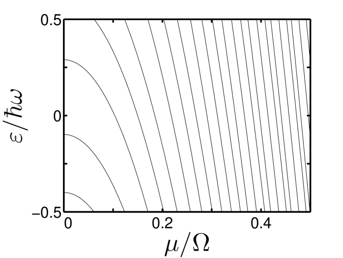
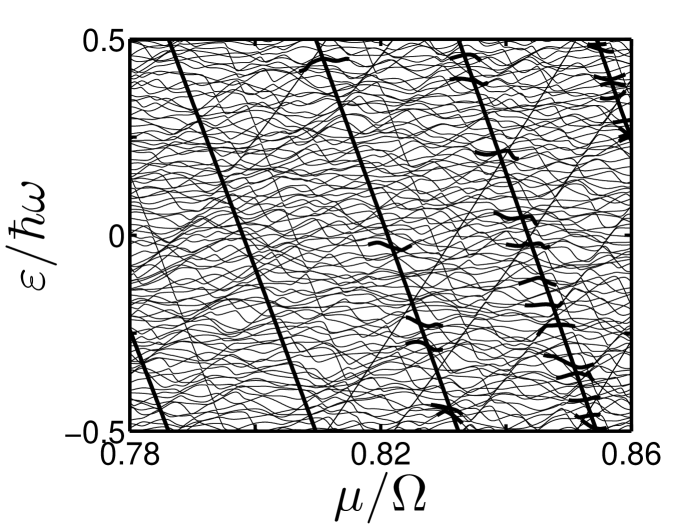
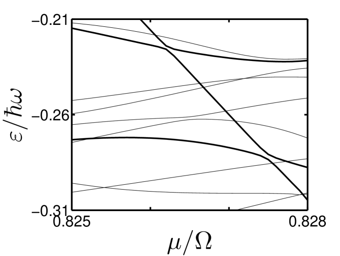
Figure 1: (a) One Brillouin zone of quasienergy eigenvalues emerging from the lowest three energy eigenstates of the undriven Josephson junction (28) with $N=100$ particles and scaled interaction strength $N\kappa/\Omega=0.95$ when subjected to forcings (30) with scaled driving frequency $\omega/\Omega=1.0$ and constant amplitude $\mu/\Omega$. On the left margin, quantum numbers $n$ are $2$, $0$, $1$ (top to bottom). (b) Magnification of a part of the quasienergy spectrum, with all eigenvalues included. The heavy line is the quasienergy emerging from the ground state of the junction (28). Short heavy line segments indicate avoided crossings with a gap larger than about $\delta\epsilon/(\hbar\omega)=10^{-3}$. (c) Further magnification confirms that the quasienergy line highlighted in (b) actually is broken by narrow avoided crossings. These anticrossings tend to become more wide with increasing driving amplitude.

In Fig. 1 we display parts of the quasienergy spectrum obtained when the system is driven with constant scaled amplitude $\mu/\Omega$, while $N=100$, $N\kappa/\Omega=0.95$, and $\omega/\Omega=1.0$; these parameters will be kept fixed in the following. The upper panel shows the quasienergies emerging from the three lowest energy eigenstates $n=0,1,2$ of the undriven junction (28), reduced to the fundamental quasienergy Brillouin zone $-1/2\leq\varepsilon/(\hbar\omega)<+1/2$, for small scaled driving amplitudes $0\leq\mu/\Omega\leq 0.5$. These quasienergy lines still appear to be smooth, providing favorable conditions for adiabatic transport. The middle panel then shows all 101 quasienergies of the system in the interval $0.78\leq\mu/\Omega\leq 0.86$; the representative associated with the ground state $n=0$ of the junction (28) has been highlighted. Actually, the corresponding Floquet state “feels” (i.e., interacts with) the “background” provided by all other states: For constant driving amplitude, the quasienergy operator

$$K^{\mu}=H_{0}+\hbar\mu\sin(\omega t)\left(a^{\dagger}_{1}a^{\phantom{\dagger}}_{1}-a^{\dagger}_{2}a^{\phantom{\dagger}}_{2}\right)+\frac{\hbar}{{\mathrm{i}}}\frac{{\mathrm{d}}}{{\mathrm{d}}t}$$ (31)

remains unchanged when swapping the two sites by interchanging the indices $1$ and $2$, and simultaneously shifting the time by half a period, $t\to t+\pi/\omega$. The Floquet functions are even or odd under this generalized parity, and eigenvalues belonging to the same parity should not cross each other, according to the von Neumann-Wigner theorem NeumannWigner29 . Therefore, about half of the apparent crossings observed in the middle panel of Fig. 1 actually are non-resolved anticrossings. This deduction is confirmed in the lower panel, which magnifies two of these avoided crossings. “Relevant” avoided crossings with a sizeable gap only occur in the strong-driving regime; avoided crossings affecting the Floquet state emerging from the ground state with a gap larger than about $\delta\varepsilon/(\hbar\omega)=10^{-3}$ have been indicated in the middle panel. Here we encounter, albeit in a relatively small system only, a pertinent consequence of the Brillouin zone structure of the quasienergy spectrum: The denseness of the quasienergies gives rise to a plethora of avoided crossings, corresponding to multiphoton-like resonances which endanger adiabatic transport. However, as long as the driving amplitude remains sufficiently small these anticrossings remain possibly even undetectably narrow, so that the Floquet state emerging from the undriven system’s many-body ground state is not strongly affected, and its quasienergy function $\varepsilon_{0}(\mu/\Omega)$ may be regarded as smooth and isolated in a coarse-grained sense Holthaus15 .

A useful means to characterize the individual many-body Floquet states is to compute their respective one-particle reduced density matrix

$$\varrho_{n}=\left(\begin{array}[]{cc}\langle a^{\dagger}_{1}a^{\phantom{\dagger}}_{1}\rangle&\langle a^{\dagger}_{1}a^{\phantom{\dagger}}_{2}\rangle\\ \langle a^{\dagger}_{2}a^{\phantom{\dagger}}_{1}\rangle&\langle a^{\dagger}_{2}a^{\phantom{\dagger}}_{2}\rangle\end{array}\right)\;,$$ (32)

and to determine the “degrees of simplicity” Leggett01

$$\eta_{n}=2N^{-2}\,{\rm tr}\,\varrho_{n}^{2}-1\;.$$ (33)

Obviously $\eta_{n}=1$ when $|u_{n}(t)\rangle$ corresponds to an $N$-fold occupied, periodically time-dependent single-particle state, i.e., to a Floquet condensate, whereas $\eta_{n}=0$ when the state is maximally fractionalized. Hence, the numerical value $0\leq\eta_{n}\leq 1$ provides a measure for the coherence of $|u_{n}(t)\rangle$.

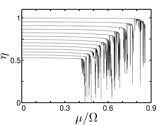
Figure 2: Degree of coherence, as defined by Eq. (33), for the Floquet states connected to the lowest energy eigenstates of the undriven junction (28) for $N=100$, $N\kappa/\Omega=0.95$, and $\omega/\Omega=1.0$. On the left margin, quantum numbers $n$ are $0,1,\ldots,12$ (top to bottom).

In Fig. 2 we depict $\eta_{n}$ for $n=0,1,\ldots,12$, again for $N=100$, $N\kappa/\Omega=0.95$, and $\omega/\Omega=1.0$. Evidently the Floquet state emerging from the undriven ground state corresponds to a periodically time-dependent Bose-Einstein condensate up to roughly $\mu/\Omega\approx 0.8$. For higher driving amplitudes the coarse-graining approach mentioned above does no longer work, the web of resonances starts to make itself felt, and the coherence is lost.

Remarkably, here the ordering of the system’s Floquet states with respect to their degree of coherence follows the quantum number $n$ of the eigenstates of the undriven junction (28). This is due to the fact that our driving frequency $\omega=\Omega$, times $\hbar$, is somewhat lower than the energy level spacing of the system (28) in the vicinity of its ground state; for other choices of $\omega$ the condensate-carrying Floquet ground state may not be connected to the unperturbed ground state $n=0$ GertjerenkenHolthaus14a ; GertjerenkenHolthaus14b .

Next, we explore the expected possibility of an adiabatic preparation of a Floquet condensate: We choose a Gaussian switch-on function

$$\mu(t)=\left\{\begin{array}[]{ll}\mu_{\rm max}\exp\left(-\frac{t^{2}}{2\sigma^{2}}\right)&,\;t\leq 0\\ \mu_{\rm max}&,\;t>0\end{array}\right.$$ (34)

with steepness parameter $\sigma$. The larger the dimensionless ratio $\sigma/T$, the longer is the time during which the system’s wave function can adjust to the changing driving amplitude.

Figure 3: Logarithm of the adiabaticity defect $1-p_{0}$, with $p_{0}=|a_{0}(0)|^{2}$, obtained when transporting the initially prepared ground state $n=0$ of the junction (28) for $N=100$ and $N\kappa/\Omega=0.95$ to the amplitude $\mu_{\rm max}/\Omega=0.8$ with the help of the switch-on function (34), again setting $\omega/\Omega=1.0$. Observe that the best adiabaticity is achieved with intermediate steepness, $\sigma/T\approx 20$. For even longer turn-on times the system undergoes sizeable Landau-Zener transitions at small avoided crossings.

We then populate the ground state $n=0$ of the undriven junction (28) at large negative times $t_{0}$, when $H_{1}(t)$ is still negligible, and solve the time-dependent Schrödinger equation with this initial condition to obtain $|\psi(t\rangle$ for $t_{0}\leq t\leq 0$, employing switch-on functions (34) with various values of the steepness $\sigma$; all calculations reported in the following start at $t_{0}=-5\sigma$. At suitable moments $t>t_{0}$ the solution $|\psi(t)\rangle$ is expanded with respect to the corresponding instantaneous Floquet states, thus obtaining their occupation probabilities $|a_{n}(t)|^{2}$. Figure 3 depicts the resulting deviation from perfect adiabaticity at $t=0$ when the final amplitude $\mu_{\rm max}/\Omega=0.8$ has been reached: If $1-|a_{0}(0)|^{2}$ were equal to zero, the initial ground state would have been transferred without loss into the connected Floquet state, in the sense of Eq. (23). Instead, one observes large deviations from adiabaticity when $\sigma$ is not longer than a few cycles; for such sudden turn-ons the wave function simply has no time to adjust itself to the forcing. As expected, these deviations are diminished rapidly when the turn-on proceeds more slowly, being smallest when the steepness parameter $\sigma$ is about $20$ cycles. However, when is $\sigma$ increased further, so that the steepness is reduced even more, the deviations from adiabaticity increase again: Now the system’s wave function does not “jump” more or less entirely over the small avoided crossings exemplified in the lower panel of Fig. 1, but undergoes sizeable Landau-Zener transitions to the anticrossing Floquet states BreuerHolthaus89b ; DreseHolthaus99 . That is, the system becomes able to resolve the multitude of avoided crossings if it is given sufficient time. Therefore, in a system with a truly macroscopic number of particles, and hence with an uncomputably dense web of anticrossing quasienergies, an “adiabatic limit” in the mathematical sence, i.e., for $\sigma/T\to\infty$, cannot be attained. Our key point is that this absence of a proper adiabatic limit does not obstruct an effectively adiabatic controllability for reasonably chosen, finite parameter speed, and moderate maximum driving amplitude.

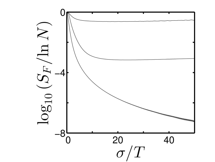
Figure 4: Floquet entropy (35), normalized to $\ln N$, resulting at $t=0$ from turn-ons (34) with $\mu_{\rm max}/\Omega=0.6$ (lower curve), $0.8$ (middle curve), and $0.9$ (upper curve). Again, $N=100$, $\omega/\Omega=1.0$, and $N\kappa/\Omega=0.95$.

To substantiate this claim, we introduce the Floquet entropy

$$S_{F}(t)=-\sum_{n}|a_{n}(t)|^{2}\ln|a_{n}(t)|^{2}$$ (35)

which is zero if only one single Floquet state is populated, and takes on its maximum value $\ln(N+1)\approx\ln N$ when all $N+1$ Floquet states are populated equally. In Fig. 4 we show the normalized entropy $S_{F}(0)/\ln N$ resulting from turn-ons with $\mu_{\rm max}/\Omega=0.6$, $0.8$, and $0.9$, respectively: As witnessed by the previous Fig. 2, for maximum driving amplitude $\mu_{\rm max}/\Omega=0.6$ the many-body wave function evolving from the undriven system’s ground state still remains in the regime where the quasienergy anticrossings cannot be resolved, so that its coherence is well preserved and the final entropy is still decreasing with increasing $\sigma$ even for “creeping” turn-ons with $\sigma/T\approx 50$; of course it has to increase eventually when $\sigma/T$ is made much larger. The curve for $\mu_{\rm max}/\Omega=0.8$ corresponds to the one plotted in Fig. 3; this case falls into the parameter regime where the system starts to “feel” the anticrossings. But for $\mu_{\rm max}/\Omega=0.9$ these anticrossings become so wide that the final Floquet entropy $S_{F}(0)$ already is comparable to $\ln N$, indicating that so many Landau-Zener transitions have taken place during the turn-on that a quite substantial fraction of the Floquet states has been populated to an appreciable degree, and the system’s coherence is destroyed more or less completely.

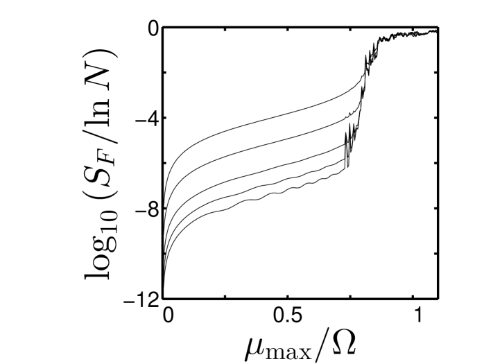
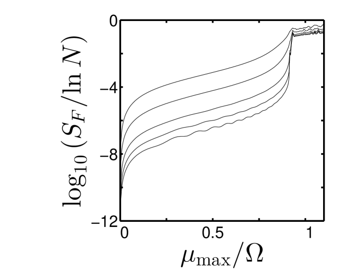
Figure 5: Floquet entropy (35), normalized to $\ln N$, resulting at $t=0$ from turn-ons (34) with steepness $\sigma/T=5$, $10$, $20$, $30$, $40$ (top to bottom). In the upper panel we have set $N=100$, as before, whereas $N=1000$ in the lower panel. In both cases, $\omega/\Omega=1.0$ and $N\kappa/\Omega=0.95$.

These three regimes of response — the effectively adiabatic regime in which the final Floquet entropy $S_{F}(0)$ is small, and decreases with increasing $\sigma$; the transition regime; and the chaotic regime in which $S_{F}(0)$ is large, and almost independent of $\sigma$ — are clearly discernible in Fig 5: Here we show $S_{F}(0)/\ln N$ as function of $\mu_{\rm max}/\Omega$ for several steepnesses $\sigma$. The upper panel, computed again for merely $N=100$ particles, allows one to identify the transition regime $0.75<\mu_{\rm max}/\Omega<0.85$; the lower panel, obtained for $N=1000$, reveals a much sharper transition at $\mu_{\rm max}/\Omega\approx 0.85$. The fact that the main features remain unchanged when going from $N=100$ to $N=1000$, while keeping $N\kappa/\Omega=0.95$ at a constant value, is not trivial, because there are two opposing tendencies GertjerenkenHolthaus14b : On the one hand, the quasienergy density in the Brillouin zone increases with $N$, leading to more avoided crossings; on the other hand, the reduction of $\kappa$ with $1/N$ implies that the individual anticrossings become more narrow. In combination, these trends still allow for an extended effectively adiabatic regime even for $N=1000$ and larger: In this regime the $N$-particle ground state of the undriven Josephson junction (28) can be adiabatically shifted, by means of a well designed, smooth turn-on of a time-periodic driving force, into the connected many-body Floquet state; according to Fig. 2, this state has the coherence properties of an $N$-fold occupied, $T$-periodic single-particle state. In short, with judiciously chosen parameters the adiabatic preparation of a Floquet condensate is possible.

IV Discussion

The exact numerical calculations presented in Sec. III refer to a highly idealized model system. Yet, they have revealed some features which we believe to be generic, and which are likely to persist in actual laboratory set-ups not necessarily involving a condensate in a driven double well. We surmise the existence of windows of opportunity, i.e., of parameter regimes enabling one to adiabatically transform a static Bose-Einstein condensate into a dynamic Floquet condensate without appreciable generation of Floquet entropy, although the denseness of the system’s quasienergy spectrum seems to forbid a naive application of the standard adiabatic theorem. This prediction, which is substantiated by Fig. 3, could be verified experimentally by subjecting a trapped Bose-Einstein condensate a to an oscillating drive with a smooth turn-on, and by swiching off the trapping potential suddenly after the maximum driving amplitude has been reached: Time-of-flight absorption images taken in the adiabatic regime then should reveal a high degree of coherence, despite the previous action of the possibly strong force.

Another observation of interest, deduced from Fig. 5, concerns the possibility that the adiabatic regime may have a rather sharp border; this is related to the recently discussed “sudden death” of a macroscopic wave function under strong forcing GertjerenkenHolthaus15 . Here we encounter a dynamically induced (instead of thermal) destruction of a condensate’s coherence which can be traced to a change of the nature of the system’s quasienergy spectrum: While the quasienergy of the state to be transported, when viewed as a function of the slowly changing parameter, is effectively smooth (that is, broken only by unresolvably narrow anticrossings) in the adiabatic regime, it becomes disrupted by a multitude of large avoided crossings in the coherence-killing chaotic regime. Thus, characteristic properties of spectra which have been investigated in great detail in the context of single-particle quantum chaos Haake10 ; Stoeckmann07 may find further, unforeseen applications in the realm of forced many-particle systems. Again, the existence of such a “chaos border” should have a clear-cut experimental signature: In a sequence of measurements of the type sketched above, performed with subsequently enhanced maximum driving strengths, one should observe a sharp coherence drop within a relatively small interval of these maximum driving amplitudes.

- (1) J. Struck, C. Ölschläger, M. Weinberg, P. Hauke, J. Simonet, A. Eckardt, M. Lewenstein, K. Sengstock, and P. Windpassinger, Phys. Rev. Lett. 108, 225304 (2012).
- (2) P. Hauke, O. Tieleman, A. Celi, C. Ölschläger, J. Simonet, J. Struck, M. Weinberg, P. Windpassinger, K. Sengstock, M. Lewenstein, and A. Eckardt, Phys. Rev. Lett. 109, 145301 (2012).
- (3) For a review, see A. Eckardt, Periodically driven lattices: From dynamic localization to artificial magnetism (in preparation).
- (4) C. V. Parker, L.-C. Ha, and C. Chin, Nature Physics 9, 769 (2013).
- (5) L.-C. Ha, L. W. Clark, C. V. Parker, B. M. Anderson, and C. Chin, Phys. Rev. Lett. 114, 055301 (2015).
- (6) G. Jotzu, M. Messer, R. Desbuquois, M. Lebrat, T. Uehlinger, D. Greif, and T. Esslinger, Nature 515, 237 (2014).
- (7) C. J. Kennedy, W. C. Burton, W. C. Chung, and W. Ketterle, Nature Physics 11, 859 (2015).
- (8) M. Weinberg, C. Ölschläger, C. Sträter, S. Prelle, A. Eckardt, K. Sengstock, and J. Simonet, Phys. Rev. A 92, 043621 (2015).
- (9) L. Jiang, T. Kitagawa, J. Alicea, A. R. Akhmerov, D. Pekker, G. Refael, J. I. Cirac, E. Demler, M. D. Lukin, and P. Zoller, Phys. Rev. Lett. 106, 220402 (2011).
- (10) D. E. Liu, A. Levchenko, and H. U. Baranger, Phys. Rev. Lett. 111, 047002 (2013).
- (11) M. D. Reichl and E. J. Mueller, Phys. Rev. A 89, 063628 (2014).
- (12) For a tutorial review, see: M. Holthaus, J. Phys. B: At. Mol. Opt. Phys. 49, 013001 (2016).
- (13) G. Floquet, Annales de l’ École Normale Supérieure 12, 47 (1883).
- (14) Ya. B. Zel’dovich, J. Exptl. Theoret. Phys. (U.S.S.R.) 51, 1492 (1966) [Sov. Phys. JETP 24, 1006 (1967)].
- (15) V. I. Ritus, J. Exptl. Theoret. Phys. (U.S.S.R.) 51, 1544 (1966) [Sov. Phys. JETP 24, 1041 (1967)].
- (16) J. S. Howland, in: Schrödinger operators: The quantum mechanical many-body problem. Lecture Notes in Physics 403, p. 100 (Springer, Berlin, 1992).
- (17) B. Gertjerenken and M. Holthaus, New J. Phys. 16, 093009 (2014).
- (18) B. Gertjerenken and M. Holthaus, Phys. Rev. A 90, 053614 (2014).
- (19) M. Holthaus and S. Stenholm, Eur. Phys. J. B 20, 451 (2001).
- (20) H. P. Breuer and M. Holthaus, Z. Phys. D 11, 1 (1989).
- (21) H P. Breuer and M. Holthaus, Phys. Lett. A 140, 507 (1989).
- (22) K. Drese and M. Holthaus, Eur. Phys. J. D 5, 119 (1999).
- (23) H. Sambe, Phys. Rev. A 7, 2203 (1973).
- (24) M. Born and V. Fock, Z. Phys. 51, 165 (1928).
- (25) T. Kato, J. Phys. Soc. Japan 5, 435 (1950).
- (26) M. V. Berry, Proc. R. Soc. Lond. A 392, 45 (1984).
- (27) B. Simon, Phys. Rev. Lett. 51, 2167 (1983).
- (28) H. J. Lipkin, N. Meshkov, and A. J. Glick, Nucl. Phys. 62, 188 (1965).
- (29) A. C. Scott and J. C. Eilbeck, Phys. Lett. A 119, 60 (1986).
- (30) G. J. Milburn, J. Corney, E. M. Wright, and D. F. Walls, Phys. Rev. A 55, 4318 (1997).
- (31) A. J. Leggett, Rev. Mod. Phys. 73, 307 (2001).
- (32) R. Gati and M. K. Oberthaler, J. Phys. B: At. Mol. Opt. Phys. 40, R61 (2007).
- (33) B. Gertjerenken and M. Holthaus, Annals of Physics 362, 482 (2015).
- (34) J. von Neumann and E. P. Wigner, Phys. Z. 30, 467 (1929).
- (35) F. Haake, Quantum Signatures of Chaos, 3rd edition (Springer-Verlag Berlin Heidelberg, 2010).
- (36) H.-J. Stöckmann, Quantum Chaos – An Introduction (Cambridge University Press, 2007).