One-dimensional frustrated plaquette compass model:
Nematic phase and spontaneous multimerization

Abstract

We introduce a one-dimensional (1D) pseudospin model on a ladder where the Ising interactions along the legs and along the rungs alternate between $X_{i}X_{i+1}$ and $Z_{i}Z_{i+1}$ for even/odd bond (rung). We include also the next nearest neighbor Ising interactions on plaquettes’ diagonals that alternate in such a way that a model where only leg interactions are switched on is equivalent to the one when only the diagonal ones are present. Thus in the absence of rung interactions the model can interpolate between two 1D compass models. The model posses local symmetries which are the parities within each $2\times 2$ cell (plaquette) of the ladder. We find that for different values of the interaction it can realize ground states that differ by the patterns formed by these local parities. By exact diagonalization we derive detailed phase diagrams for small systems of $L=4$, 6 and 8 plaquettes, and use next $L=12$ to identify generic phases that appear in larger systems as well. Among them we find a nematic phase with macroscopic degeneracy when the leg and diagonal interactions are equal and the rung interactions are larger than a critical value. By performing a perturbative expansion around this phase we find indeed a very complex competition around the nematic phase which has to do with releasing frustration in this range of parameters. The nematic phase is similar to the one found in the two-dimensional compass model. For particular parameters the low-energy sector of the present plaquette model reduces to a 1D compass model with spins $S=1$ which suggests that it realizes peculiar crossovers within the class of compass models. Finally, we show that the model can realize phases with broken translation invariance which can be either dimerized, trimerized, etcetera, or completely disordered and highly entangled in a well identified window of the phase diagram.

I Introduction

Entanglement in spin models is one of the central topics in modern condensed matter theory Ami08 . It is frequently accompanied by frustration of exchange interactions Nor09 ; Bal10 . However, frustration alone is not sufficient to generate entanglement but in many cases it triggers entangled excited or ground states. Some models without entanglement are exactly solvable in two dimensions, as for instance the fully frustrated two-dimensional (2D) Ising model of Villain Vil77 with the reversed sign of exchange interaction along every second column with respect to the unfrustrated square lattice, and its generalization with periodically distributed frustrated bonds along more distant columns Lon80 .

In contrast, the 2D compass model Nus15 , with competing $X_{i}X_{j}$ and $Z_{i}Z_{j}$ interactions between $S=1/2$ pseudospins ($X_{i}$ and $Z_{i}$ are Pauli matrices) along horizontal and vertical bonds in the square lattice, is quantum and has intrinsic entanglement which can be reliably treated only by advanced many-body methods Che07 ; Oru09 , including quantum Monte Carlo Wen08 , multi-configurational entanglement renormalization ansatz Cin10 , or tensor networks at finite temperature Cza16 . The latter approach allowed to confirm that long-range order develops in the 2D quantum compass model at finite temperature, in analogy to the 2D classical Ising model, without or with frustrated interactions Vil77 ; Lon80 . Moreover, the symmetry properties of the 2D compass model are responsible for certain relations between the correlations functions which may be viewed as hidden order You10 ; Brz10 .

Recent interest in the compass models is motivated by several developments: (i) investigating quantum phase transitions Che07 ; Oru09 ; Cin10 ; (ii) its relation to $p+ip$ superconductivity Nus05 ; (iii) recently confirmed prospect of topological quantum computing Kit03 ; Dou05 ; Dor05 ; Dus09 — it could be realized in nanoscopic systems where perturbing Heisenberg interactions do not destroy the nematic order in the lowest energy excited states Tro10 while the ground state remains ordered also at finite temperature Pla15 ; (iv) order and excitations in case of compass interactions on a frustrated checkerboard lattice Nas12 ; (v) spin-orbital physics in transition metal oxides with active orbital degrees of freedom Kug82 ; Fei97 ; Hfm ; Tokura ; Kha01 ; Ver04 ; Ole05 ; Kha05 ; Ulr06 ; Hor08 ; Kru09 ; Karlo ; Woh11 ; Ole12 ; Brz12 ; Cza15 ; Ave13 ; Brz15 ; (vi) its realization in iridates with strong spin-orbit coupling Jac09 , leading to the compass interactions on the triangular lattice Jac15 or to the exactly solvable Kitaev model on the honeycomb lattice Kit06 ; Bas07 , and (vii) its experimental realizations in optical lattices Mil07 . In case of ferromagnetic (FM) spin-orbital systems entanglement is absent Ole06 and one finds here quantum orbital models vdB04 ; vdB99 ; Fei05 ; Ish05 ; Dag08 ; Ryn10 ; Wro10 ; Dag10 ; Tro13 ; Che13 . The 2D compass model is their generic representation and its interactions stand for directional orbital interactions between $e_{g}$ or $t_{2g}$ orbitals on the 2D square or on three-dimensional (3D) cubic lattice. While both $e_{g}$ and $t_{2g}$ orbital models are distinct, none of them reduces to the compass model Nus15 ; Wen11 which is more universal and stands for the paradigm of directional interactions in the orbital physics vdB99 ; vdB04 ; Fei05 ; Ish05 ; Dag08 ; Ryn10 ; Wro10 ; Dag10 ; Tro13 ; Che13 .

In spite of their conceptual simplicity, only very few quantum orbital models are exactly solvable. Among them the Kitaev model on the honeycomb lattice is the most prominent one as it describes a spin liquid with only nearest neighbor (NN) spin correlations Kit06 ; Bas07 . Recently considerable attention attracted also the one-dimensional (1D) compass model which is exactly solvable by the mapping on the transverse Ising model Brz07 . As the 2D compass model, it includes only two spin components and the ground state is highly degenerate. This triggers various phase transitions when the interactions are tuned Sun09 . By investigating the block entanglement entropy in the four ground-state phases it has been found that the changes of entanglement signal the second-order rather than the first-order transitions Eri09 . Further insights into the mechanism of quantum phase transitions were obtained by matrix product state approach Liu12 ; Wan15 . Furthermore, the exact solution was generalized to the case with a finite transverse field Jaf11 which destabilizes the orbital-liquid ground state with macroscopic degeneracy and rather peculiar specific heat and polarization behavior of the 1D compass model follows from highly frustrated interactions You14 .

Another exactly solvable case is the compass model on a ladder with leg and rung interactions satisfying the same directional pattern as in the 2D model Brz09 . In contrast, the 1D plaquette orbital model with a topology of a ladder introduced recently Brz14 is not exactly solvable but transforms to an effective 1D spin model in a magnetic field, with spin dimers that replace plaquettes and are coupled along the chain by three-spin interactions. This model is motivated by the 2D plaquette orbital model Wen09 ; Bis10 and has very interesting properties as the quantum effects are of purely short-range nature which makes it possible to estimate the ground state energy in the thermodynamic limit from the exact diagonalization of finite clusters.

In the present paper we investigate a generalization of the 1D plaquette compass model Brz14 with the diagonal pseudospin interactions added within each plaquette. We present the phase diagrams obtained by exact diagonalization for finite systems with periodic boundary conditions (PBCs) which contain generic phases that are expected to appear for any system size. This model interpolates between two 1D compass models in absence of rung interactions. As we show below, the nematic phase found in this frustrated plaquette orbital model is similar to the one established for the 2D case Wen09 which indicates that the present model realizes the paradigm of dimensional crossover within the class of compass models.

The paper is organized as follows: in Sec. II we introduce the frustrated $Cx$-$Cz$ Hamiltonian and derive its block-diagonal form making use of its local symmetries. Its symmetry line in the parameter space is explored in Sec. III. Next we present a competition between different classical states for a single plaquette in Sec. IV.1 and show that this can be used as a guideline to understand the complex quantum phase diagram for a generic case of $L$ interacting plaquettes, as shown for $L=4$ in Sec. IV.2 where we also visualize the configurations found there. In Sec. IV.3 we present the phase diagram for $L=4$ in the anisotropic case when all the ZZ interaction are slightly weaker than the XX ones. Phase diagrams for larger systems with $L>4$ are investigated in Sec. V — in Sec. V.1 we show the detailed phase diagram for a ladder consisting of $L=$6 plaquettes and its configurations, while Secs. V.2 and V.3 concentrate on the evolution of phase diagram with increasing $L$ and identification of generic phases using large ladders with $L=8$ and $L=12$. Section VI is devoted to phase competition in the vicinity of the nematic phase and we study the behavior of the energy levels when this phase is approached using perturbative expansion up to fourth order. Finally, in Sec. VII.1 we quantify the entanglement of the effective dimers in symmetry subspaces for the systems of the sizes $L=4$ and $L=6$. In Sec. VII.2 we do the same for plaquettes in initial physical basis. The summary and conclusions are given in Sec. VIII. The paper is supplemented with one Appendix in which we show the relation between the spin transformation that we use to block-diagonalize the present model and the one which was used before for a simpler $Cx$–$Cz$ model Brz14 .

II Hamilonian and its symmetries

We consider the Hamiltonian of the 1D plaquette compass $Cx$–$Cz$ model which can be written as follows,

$${\cal H} = \sum_{i=1}^{L}\left\{J_{{\rm rung}}X_{i,2}X_{i,3}+J_{{\rm leg}}\left(X_{i,1}X_{i,2}+X_{i,3}X_{i,4}\right)\right\}$$ (1)

$$+ J_{{\rm diag}}\sum_{i=1}^{L}\left(X_{i,1}X_{i,3}+X_{i,2}X_{i,4}\right)$$

$$+ \sum_{i=1}^{L}\left\{J_{{\rm rung}}Z_{i,1}Z_{i,4}+J_{{\rm leg}}\left(Z_{i,1}Z_{i+1,2}+Z_{i,4}Z_{i+1,3}\right)\right\}$$

$$+ J_{{\rm diag}}\sum_{i=1}^{L}\left(Z_{i,1}Z_{i+1,3}+Z_{i,4}Z_{i+1,2}\right),$$

where $X_{i,p}$ and $Z_{i,p}$ are the $\sigma^{x}$ and $\sigma^{z}$ Pauli matrices for plaquette $i=1,\dots,L$ at site $p=1,2,3,4$, see Fig. 1. We consider all exchange interactions positive, i.e., antiferromagnetic (AF). A simpler $Cx$–$Cz$ model considered in Ref. Brz14 can be recovered by setting $J_{{\rm rung}}=J_{{\rm leg}}$ and $J_{{\rm diag}}=0$. Here and below we assume PBCs of the form $Z_{L+1,2}=Z_{1,2}$ and $Z_{L+1,3}=Z_{1,3}$.

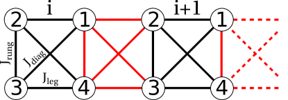
Figure 1: Schematic view of the Hamiltonian of the 1D plaquette compass $Cx$–$Cz$ model, see Eq. (1). Black (red) lines stand for the XX (ZZ) bonds connecting first and second neighbors. The system is naturally divided into four-site cells (plaquettes) that are labeled by $i=1,2,\dots,L$ and which carry internal site index $p=1,2,3,4$.

There are two types of the symmetry operators specific to the model (1), namely

$$P_{i}^{z} = Z_{i,1}Z_{i,2}Z_{i,3}Z_{i,4},$$

$$P_{i}^{x} = X_{i,1}X_{i,4}X_{i+1,2}X_{i+1,3}.$$ (2)

Following the spin transformations derived in Ref. Brz14 we can find a block-diagonal form of the Hamiltonian ${\cal H}$ (1) in the common eigenspace of the symmetry operators. Here we will use an alternative form of such transformation, as we consider it more suitable to treat the present frustrated (generalized) problem, namely:

$$X_{i,1} = r_{i}^{\star},$$

$$X_{i,2} = r_{i}^{\star}s_{i}\tau_{i,2}^{x}\tau_{i,3}^{x},$$

$$X_{i,3} = r_{i}^{\star}s_{i}\tau_{i,3}^{x},$$

$$X_{i,4} = r_{i}^{\star}s_{i}\tau_{i+1,2}^{x},$$ (3)

and

$$Z_{i,1} = s_{i}^{\star}\tau_{i,3}^{z},$$

$$Z_{i,2} = s_{i-1}^{\star}\tau_{i,2}^{z},$$

$$Z_{i,3} = s_{i-1}^{\star}r_{i}\tau_{i,2}^{z}\tau_{i,3}^{z},$$

$$Z_{i,4} = s_{i}^{\star}.$$ (4)

Here $\tau_{i,2/3}^{x/z}$ are new Pauli operators at plaquette $i$ and sites $2$ and $3$ within the plaquette and $r_{i}$ and $s_{i}$ are the symmetry operators, namely

$$r_{i}\equiv P_{i}^{z} = Z_{i,1}Z_{i,2}Z_{i,3}Z_{i,4},$$

$$s_{i}\equiv P_{i}^{x} = X_{i,1}X_{i,4}X_{i+1,2}X_{i+1,3},$$ (5)

and $r_{i}^{\star}$ , $s_{i}^{\star}$ are the anticommuting partners of these operators that can be expressed in terms of initial Pauli operators as,

$$r_{i}^{\star} = X_{i,1},$$

$$s_{i}^{\star} = Z_{i,4}.$$ (6)

These operators will not be needed: $r_{i}^{\star}$ and $s_{i}^{\star}$ do not appear in the block-diagonal form of the Hamiltonian and $r_{i}$ and $s_{i}$ are good quantum numbers taking the values of $\pm 1$. The transformations of Eqs. (3) and (4), whatever complicated they may be, are reversible. The inverse transformations read:

$$\tau_{i,2}^{x} = X_{i,2}X_{i,3},$$

$$\tau_{i,3}^{x} = X_{i,3}X_{i,4}X_{i+1,2}X_{i+1,3},$$ (7)

and

$$\tau_{i,2}^{z} = Z_{i,2}Z_{i-1,4}$$

$$\tau_{i,3}^{z} = Z_{i,1}Z_{i,4},$$ (8)

completed by the relations of Eqs. (5) and (6). Note that however $r_{i}$ and $s_{i}$ can be alternatively called $r_{i}\equiv\tau_{i,1}^{z}$ and $s_{i}\equiv\tau_{i,4}^{x}$, as they commute with the pseudospins $\tau_{i,2}^{x/z}$ and $\tau_{i,3}^{x/z}$. This does not automatically imply that $r_{i}^{\star}$ and $s_{i}^{\star}$ can be indeed identified with $\tau_{i,1}^{x}$ and $\tau_{i,4}^{z}$, we find that $r_{i}^{\star}$ anticommutes with $\tau_{i,3}^{z}$ and $s_{i}^{\star}$ with $\tau_{i,3}^{x}$. The block diagonal Hamiltonian has the following form:

$${\cal H} = \sum_{i=1}^{L}\left\{J_{{\rm rung}}\tau_{i,2}^{x}+J_{{\rm leg}}\left(s_{i}\tau_{i,2}^{x}\tau_{i,3}^{x}+\tau_{i,3}^{x}\tau_{i+1,2}^{x}\right)\right\}$$ (9)

$$+ J_{{\rm diag}}\sum_{i=1}^{L}\left(s_{i}+\tau_{i,2}^{x}\tau_{i+1,2}^{x}\right)\tau_{i,3}^{x}$$

$$+ \sum_{i=1}^{L}\left\{J_{{\rm rung}}\tau_{i,3}^{z}+J_{{\rm leg}}\left(r_{i}\tau_{i,2}^{z}\tau_{i,3}^{z}+\tau_{i,3}^{z}\tau_{i+1,2}^{z}\right)\right\}$$

$$+ J_{{\rm diag}}\sum_{i=1}^{L}\left(1+r_{i}\tau_{i-1,3}^{z}\tau_{i,3}^{z}\right)\tau_{i,2}^{z}.$$

From the computational point of view it is worth to notice that thanks to the symmetries we reduce the number of quantum degrees of freedom by half, i.e., instead of four initial Pauli operators $\left\{X_{i,1},X_{i,2},X_{i,3},X_{i,4}\right\}$ and their anticommuting partners per each plaquette (see Fig. 1), we now have only two of them, $\left\{\tau_{i,2}^{z},\tau_{i,3}^{z}\right\}$, with anticommuting partners and two good quantum numbers $\left\{r_{i},s_{i}\right\}$ taking values $\pm 1$. Thus instead of plaquettes with internal site index $p=1,2,3,4$ we now deal with dimers with $p=2,3$. From the fundamental point of view the specific pattern of the $\left\{r_{i},s_{i}\right\}$ Ising spins is an important characterization of model’s ground state at given values of the interactions, as we shall see further on.

Note that in the absence of diagonal interaction, i.e., at $J_{{\rm diag}}=0$, the model is equivalent to the 1D XY model in the external XY field. To see it clearly one can redefine the Pauli operators to get rid of $p=2,3$ indices and gauge away the $r_{i}$ and $s_{i}$ phase from the interaction term (strictly speaking this can be done completely only for an open chain so we neglect here the closing $\langle L,1\rangle$ bond). To do this we use a following transformation:

$$\tau_{i,2}^{x} = s_{1}s_{2}s_{3}\dots s_{i-1}\tau^{\prime}{}_{2i-1}^{x},$$

$$\tau_{i,3}^{x} = s_{1}s_{2}s_{3}\dots s_{i}\tau^{\prime}{}_{2i}^{x},$$ (10)

and

$$\tau_{i,2}^{z} = r_{1}r_{2}r_{3}\dots r_{i-1}\tau^{\prime}{}_{2i-1}^{z},$$

$$\tau_{i,3}^{z} = r_{1}r_{2}r_{3}\dots r_{i}\tau^{\prime}{}_{2i}^{z},$$ (11)

to get

$${\cal H}^{\prime}_{{\rm OBC}}\!\left(J_{{\rm diag}}\!=\!0\right) \!=\! J_{{\rm rung}}\!\sum_{i=1}^{L}\left(R_{i}\tau^{\prime}{}_{2i}^{z}\!+\!S_{i-1}\tau^{\prime}{}_{2i-1}^{x}\right)$$ (12)

$$\!+\! J_{{\rm leg}}\!\sum_{i=1}^{2L-1}\!\left(\tau^{\prime}{}_{i}^{z}\tau^{\prime}{}_{i+1}^{z}\!+\!\tau^{\prime}{}_{i}^{x}\tau^{\prime}{}_{i+1}^{x}\right)\!,$$

with

$$R_{i} \equiv r_{1}r_{2}r_{3}\dots r_{i}.$$

$$S_{i-1} \equiv s_{1}s_{2}s_{3}\dots s_{i-1}.$$ (13)

Here the chain has open boundary conditions (OBC). Clearly the interaction part is the XY model that can be solved by a Jordan-Wigner transformation to get a solution in terms of free fermions with cosine dispersion. On the other hand, the linear part makes the model unsolvable as it becomes nonlocal and of infinite order in the thermodynamic limit after the transformation. Nevertheless, we find the $Cx$–$Cz$ model written in this form simpler than in the original form introduced in Ref. Brz14 — see the Appendix A for the transformation linking these two forms.

Another interesting limit is when $J_{{\rm rung}}=0$ and either $J_{{\rm leg}}=0$ or $J_{{\rm diag}}=0$. Looking at Fig. 1 one can easily see that in this limit the system splits into two independent subsystems and each of them is described by the so-called 1D compass model Brz07 , with XX and ZZ interactions alternating on even/odd bonds. Away from these points the two 1D compass models start to interact in a very complex way.

III High symmetry line

Apart from the local parities which are the symmetries of the model for any choice of its exchange parameters $J$’s, there is a special line in the parameter space, namely

$$J_{{\rm leg}}=J_{{\rm diag}},$$ (14)

where the model has extra symmetries. These are interchanges of the two spins located at every rung of the ladder in Fig. 1 — it is easy to notice that such an operation done on a single rung will interchange leg and diagonal bonds within the two plaquettes adjacent to this rung. When Eq. (14) is obeyed, this has no effect on Hamiltonian (1). Such interchange for a $(2,3)$ rung can be realized by a spin-interchange operator known from the so-called Kumar model Kum13 , i.e.,

$${\cal X}_{i}^{2,3}=\frac{1}{2}\left(1+\vec{\sigma}_{i,2}\cdot\vec{\sigma}_{i,3}\right),$$ (15)

where $\vec{\sigma}_{i,p}=\{X_{i,p},Y_{i,p},Z_{i,p}\}$. Similarly one can define the spin interchange operator ${\cal X}_{i}^{1,4}$ for rungs $(1,4)$.

If Eq. (14) applies, the Hamiltonian commutes with ${\cal X}_{i}^{2,3}$ and ${\cal X}_{i}^{1,4}$ for every $i$, whose spectrum consists of one eigenvalue $\lambda_{s}=-1$ for a spin singlet on a rung and three eigenvalues $\lambda_{t}=1$ for a spin triplet. This knowledge can be used to rewrite the Hamiltonian of Eq. (1) at constraint Eq. (14) in the form of ${\cal H}_{{\rm sym}}\equiv{\cal H}(J_{{\rm leg}}=J_{{\rm diag}})$ given by a following equation,

$${\cal H}_{{\rm sym}} = 2J_{{\rm rung}}\sum_{i=1}^{L}\left\{\left(S_{i,2}^{x}\right)^{2}+\left(S_{i,1}^{z}\right)^{2}-1\right\}$$ (16)

$$+ 4J_{\rm leg}\sum_{i=1}^{L}\left(S_{i,2}^{x}S_{i,1}^{x}+S_{i,1}^{z}S_{i+1,2}^{z}\right),$$

where $S_{i,3/4}^{x/z}$ are the spin $S=1$ or $S=0$ operators being the sums of two $S=1/2$ spin operators on every rung, i.e.,

$$S_{i,2}^{x}=\frac{1}{2}\left(X_{i,2}+X_{i,3}\right) ,\quad S_{i,2}^{z}=\frac{1}{2}\left(Z_{i,2}+Z_{i,3}\right),$$

$$S_{i,1}^{x}=\frac{1}{2}\left(X_{i,1}+X_{i,4}\right) ,\quad S_{i,1}^{z}=\frac{1}{2}\left(Z_{i,1}+Z_{i,4}\right).$$ (17)

The spin-interchange symmetry present in ${\cal H}_{{\rm sym}}$ guarantees that the total spin $S$ on every site $(i,2)$ and $(i,1)$ is a good quantum number. Note that in analogy to the previous Section we mapped a ladder Hamiltonian onto a model of dimerized chain but here the building blocks are $S=1$ or $S=0$ spins. This new Hamiltonian still has the parity symmetries which are now given by

$$P_{i}^{z} = \left(2\left(S_{i,2}^{z}\right)^{2}-1\right)\left(2\left(S_{i,1}^{z}\right)^{2}-1\right),$$ (18)

$$P_{i}^{x} = \left(2\left(S_{i,1}^{x}\right)^{2}-1\right)\left(2\left(S_{i+1,2}^{x}\right)^{2}-1\right),$$ (19)

whose meaning is now the parity of number of $S_{i}^{z}=0$ or $S_{i}^{x}=0$ eigenvalues on every $(2,1)$ or $(1,2)$ bond respectively.

Note that ${\cal H}_{{\rm sym}}$ has a degenerate manifold of very simple eigenstates with energy $E_{0}=-2J_{rung}L$ and degeneracy $d=2^{2L}$. These states we construct by putting on every site $(i,2)$ either total spin $S=0$ or spin $S=1$ with $S_{i,2}^{x}=0$ and on every site $(i,1)$ either total spin $S=0$ or spin $S=1$ with $S_{i,1}^{z}=0$. For the original ladder this means that on every rung $(2,3)$ we put a spin singlet or a spin triplet with zero projection on $x$ spin axis and on every rung $(1,4)$ we put a spin singlet or a spin triplet with zero projection on $z$ spin axis. Equivalently one can take a symmetric or antisymmetric combination of singlet and triplet and then for every rung $(2,3)$ we can choose between states $\left|\leftarrow\rightarrow\right\rangle$ and $\left|\rightarrow\leftarrow\right\rangle$ and for every rung $(1,4)$ we can have either $\left|\uparrow\downarrow\right\rangle$ or $\left|\downarrow\uparrow\right\rangle$. In this way we can produce $2^{2L}$ rung-product states with energy $E_{0}$. Such states belong to the ground state manifold of the model with the constraint Eq. (14) and large enough $J_{{\rm rung}}$, and we will call them nematic in the following Sections.

Finally, we note that by setting $J_{{\rm rung}}=0$ in Eq. (16), we get a Hamiltonian whose low-energy sector realizes a 1D compass model with spins $S=1$. Combining Eqs. (9) and (16) at $J_{{\rm rung}}=0$ we see that the present plaquette model realizes a crossover within a class of 1D compass models — setting $J_{{\rm leg}}=1$ and increasing $J_{{\rm diag}}$ from 0 to 1 changes spins $S=1/2$ to spins $S=1$. We note that the $S=1$ 1D compass model was studied before You13 and it was shown that for such a choice of parameter values as here the ground state of the model is unique, disordered and gapped. We also found that it is strongly dimerized, i.e., looking at two-point correlation functions only the correlations that enter the Hamiltonian (16) are non-vanishing.

IV Possible quantum phases

IV.1 A single plaquette with frustration

The ground state of the model given by the block-diagonal Hamiltonian of Eq. (9) can occur in different subspaces of the symmetry operators (i.e., different diagonal blocks) labeled by the quantum numbers $\left\{r_{1},\dots,r_{L},s_{1},\dots,s_{L}\right\}$, depending on the values of exchange parameters, $\{J_{{\rm rung}},J_{{\rm leg}},J_{{\rm diag}}\}$. This is a more complex situation than in the case of unfrustrated $Cx$–$Cz$ model where the ground state was found always in the subspace $r_{i}\equiv s_{i}\equiv 1$ Brz14 . The difference is a manifestation of the intrinsic frustration induced by the diagonal bonds.

Let us consider first a single (open) $Z$-plaquette shown in Fig. 1, described by a $4$-site Hamiltonian of the form,

$${\cal H}_{\Box} = J_{{\rm rung}}Z_{2}Z_{3}+J_{{\rm leg}}\left(Z_{1}Z_{2}+Z_{3}Z_{4}\right)$$ (20)

$$+ J_{{\rm diag}}\left(Z_{1}Z_{3}+Z_{2}Z_{4}\right),$$

where pseudospins at sites $i=1$ and $i=4$ do not interact as this bond belongs to the next plaquette, see Fig. 1. We set a constraint in the parameter space,

$$J_{{\rm diag}}=2-J_{{\rm leg}},$$ (21)

and we change $J_{{\rm leg}}$ in the interval $0\leq J_{{\rm leg}}\leq 2$ to interpolate between the two unfrustrated $Cx$–$Cz$ models. Equation (21) serves also to determine the units of dimensionless exchange parameters. Plaquette frustration vanishes when $J_{{\rm diag}}=0$, or in the equivalent limit when $J_{{\rm leg}}=0$ (but $J_{{\rm diag}}=2$) — in both limits the plaquette spins form an open chain and one recovers a unit of the unfrustrated $Cx$–$Cz$ model of Ref. Brz14 . All eigenstates are classical and have degeneracy $d=2$ (with equivalent configurations obtained by reversing all spins).

One can easily check that three distinct configurations exist which become ground states in various regions of parameters:
(i) In the area of $J_{{\rm rung}}\leq 2\left(1-\left|1-J_{{\rm leg}}\right|\right)$, the pseudospin configuration in the ground state is the one that satisfies leg and diagonal bonds but the rung bond is frustrated. This state is,

$$\left|\psi_{0}\right\rangle=\left|\uparrow\right\rangle_{1}\left|\downarrow\right\rangle_{2}\left|\downarrow\right\rangle_{3}\left|\uparrow\right\rangle_{4}.$$ (22)

(ii) For stronger $J_{{\rm rung}}>2\left(1-\left|1-J_{{\rm leg}}\right|\right)$ and $J_{{\rm leg}}<1$, one finds the ground state that optimizes only rung and diagonal bonds, namely

$$\left|\psi_{-1}\right\rangle=\left|\downarrow\right\rangle_{1}\left|\downarrow\right\rangle_{2}\left|\uparrow\right\rangle_{3}\left|\uparrow\right\rangle_{4}.$$ (23)

(iii) Finally, for $J_{{\rm rung}}>2\left(1-\left|1-J_{{\rm leg}}\right|\right)$ and $J_{{\rm leg}}>1$ we find the ground state that optimizes only rung and leg bonds which is

$$\left|\psi_{1}\right\rangle=\left|\uparrow\right\rangle_{1}\left|\downarrow\right\rangle_{2}\left|\uparrow\right\rangle_{3}\left|\downarrow\right\rangle_{4}.$$ (24)

The states (23) and (24) are degenerate along the line $J_{{\rm leg}}=1$ for $J_{{\rm rung}}>2$ in Fig. 2. The lines between the $|\psi_{0}\rangle$ and $|\psi_{1}\rangle$ ($|\psi_{-1}\rangle$) states set the stage and different phases of a ladder consisting of $Z$ and $X$ plaquettes presented in Fig. 1 develop around them, as we show below. We can expect that in the quantum many-body regime the intracell frustration discussed here will result in very non-trivial configurations.

IV.2 Phase diagram for a ladder of $L=4$ plaquettes

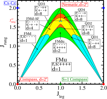
Figure 2: Ground state phase diagram for a $L=4$ plaquette ladder with PBCs as function of $J_{{\rm leg}}$ and $J_{{\rm rung}}$. The exchange on diagonal bonds $J_{{\rm diag}}$ is set following Eq. (21). The ground states (phases) are shaded in color or white and labeled according to their symmetry patterns $\left\{r_{1},\dots,r_{4};s_{1},\dots,s_{4}\right\}$, which are indicated together with their degeneracies $d$. Red dots are the 1D compass points, blue dots indicate the simple $Cx$–$Cz$ states and green dot is $S=1$ 1D compass point. The critical value $J_{{\rm rung}}^{{\rm cr}}$ for a nematic state is indicated by horizontal line at $J_{{\rm leg}}=1.0$. The boundaries separating classical states $\{\psi_{0},\psi_{-1},\psi_{1}\}$ obtained for a single frustrated $Z$-plaquette (20) are indicated by thin dashed lines.

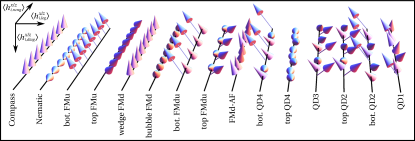
Figure 3: Visualization of the configurations which characterize different types of order in the phase diagram of Fig. 2. The solid lines indicate both the system itself and different phases or different domains of one phase which are labeled below. Arrows show the strength of the XX or ZZ interactions within consecutive plaquettes of the ladder such that their 3D components correspond to the ground-state average of the rung, leg and diagonal interactions denoted as $\langle h_{i,{\rm rung}}^{x/z}\rangle$, $\langle h_{i,{\rm leg}}^{x/z}\rangle$, and $\langle h_{i,{\rm diag}}^{x/z}\rangle$, respectively. The reference frame is given in the left top corner. Arrows along the solid lines mean that only rung interactions are non-zero, vertical arrows mean diagonal interactions, and horizontal ones on the legs only.

Indeed, in Fig. 2 we find a complex phase diagram found for a system of $L=4$ plaquettes with PBCs, containing $10$ different pseudospin configurations. All the phase boundaries mark the level crossings between the ground states from the different invariant subspaces of the Hamiltonian (1) labeled by the quantum numbers $\{r_{i},s_{i}\}$. The phase diagrams were obtained in the following way: first the phase space was discretized by a sufficiently dense lattice of points (typically $100\times 100$ points for $0\leq J_{{\rm leg}}\leq 1$ and $0\leq J_{{\rm leg}}\leq 2.2$) and for every point all the symmetry-nonequivalent subspaces were searched for the ground state to found the one with the lowest energy. Then, knowing what the phases are and how approximately they are located, the bisection algorithm was used to establish smooth boundaries between them. The dominant one was found before in the unfrustrated $Cx$–$Cz$ model, where $r_{i}\equiv s_{i}\equiv 1$. This phase we call FMu because $\{r_{i}\}$ and $\{s_{i}\}$ variables can be seen as Ising spins that are here in the FM configuration, all pointing up. This phase consists of two parts, the bottom and the top one. These parts are separated by a window of other configurations that stem from the compass points located in the bottom corners of the phase diagram. This window contains the classical phase boundaries discussed for a single plaquette in Sec. IV.1 and ends exactly at its critical point $(J_{{\rm leg}},J_{{\rm rung}})=(1.0,2.0)$.

Firstly, we note that the diagram is symmetric around the high-symmetry line $J_{{\rm leg}}=1$ starting from the $S=1$ compass point at $J_{{\rm rung}}=0$, which is deeply embedded in the FMu phase. Going up from this point we increase the values of the quadrupolar external fields in the high-symmetry Hamiltonian (16) and in the end we leave the FMu phase. Note that the ground state remains gapped along the whole $J_{{\rm leg}}=1$ line as it was at $J_{{\rm rung}}=0$. Moving left or right from this line we lower the symmetry of the problem - the $S=1$ or $S=0$ spins placed on every rung of the ladder dissociate into pairs of spins $S=1/2$ up to extreme case of compass points with exponential degeneracy at $J_{{\rm leg}}=0$ and $J_{{\rm rung}}=0$. This ’quenching’ of pairs of spins $S=1/2$ is similar to the formation of $J=0$ singlets out of spins $S=1/2$ and orbital moments $L=1/2$ in presence of strong spin-orbit coupling Jac09 .

In the narrow shoulders of the window starting from $J_{{\rm rung}}=0$ and either $J_{{\rm leg}}=0$ or $J_{{\rm leg}}=2.0$ we find two wedges of the FMd phase being exactly opposite to the FMu configuration, where all the symmetries have $-1$ eigenvalues. This phase is stable for not too large $J_{{\rm rung}}$ and away from the high symmetry point $J_{{\rm leg}}=J_{{\rm diag}}=1.0$. Quite surprisingly tiny bubbles of this phase can be found at the onset of the phase that we call nematic, exactly at $J_{{\rm leg}}=J_{{\rm diag}}=1.0$ and $J_{{\rm rung}}=J_{{\rm rung}}^{\rm cr}\simeq 1.664$. Centrally around $J_{{\rm leg}}=1$ at the very top and bottom of the window we find a phase which is partially FMu and FMd, where $r_{i}\equiv-1$ and $s_{i}\equiv 1$, namely the FMdu phase. This configuration is doubly degenerate because here is is permitted to uniformly interchange $r_{i}$ and $s_{i}$ quantum numbers and set $r_{i}\equiv 1$ and $s_{i}\equiv-1$.

More generally, the main source of degeneracies found in the phase diagram of Fig. 2 is the invariance of the block diagonal Hamiltonian of Eq. (9) with respect to translations and to $\{r_{i}\}\leftrightarrow\{s_{i}\}$ interchange. Because of this we are always allowed to cyclically translate the symmetry quantum numbers, i.e., going from the subspace $\left\{r_{1},\dots,r_{L};s_{1},\dots,s_{L}\right\}$ to $\left\{r_{L},r_{1}\dots,r_{L-1};s_{L},s_{1},\dots,s_{L-1}\right\}$ will not affect the energies. Similarly, we are allowed to translate the initial ladder of Fig. 1 by a one lattice spacing along the ladder legs provided that we also interchange all $X$ operators with the $Z$ ones. Thus going from the subspace $\left\{r_{1},\dots,r_{L};s_{1},\dots,s_{L}\right\}$ to $\left\{s_{L},s_{1},s_{2}\dots,s_{L-1};r_{1},\dots,r_{L}\right\}$ will not affect the energies as long as the $X$- and $Z$-bonds are equivalent. For simplicity this operation on the $\left\{r_{i},s_{i}\right\}$ subspace labels will be called the $r\leftrightarrow s$ interchange, keeping in mind that there is also a translation of the $s_{i}$ quantum numbers involved. Note that a very similar discussion concerns the analogous $\{r_{i},s_{i}\}$ quantum numbers in the 2D compass model, see Refs. Brz10 .

Going further towards the center of the window in the phase diagram of Fig. 2 we find the last ordered phase which is the FMd-AF one. In this phase the $\{r_{i}\}$ quantum numbers are all equal to $-1$ as in FMd phase but the $s_{i}$ ones are alternating as in the AF state, hence we use the label AF. This phase has a degeneracy of $d=8$ coming both from translation and the $r\leftrightarrow s$ interchange discussed above. In the similar area of the phase diagram we find a phase with no particular order in the eigenvalues of the symmetries which we call QD4, meaning quantum disorder. There are three other phases of this type, QD1-QD3, but all of them are stable only in tiny regions of the phase diagram, i.e., close to quantum critical points where three different phases meet.

Finally, we find special phases of measure zero in the phase diagram which have macroscopic degeneracy that cannot be explained only by the translation and the $r\leftrightarrow s$ interchange symmetry. These are the already mentioned compass points where we recover the degeneracy of two independent 1D compass models $d=\left(2^{L-1}\right)^{2}$ Brz07 , and less expected nematic phase with degeneracy $d=2^{2L}$. In the latter phase the degeneracy comes from the fact that both leg and diagonal interactions in this phase have zero expectation value and only the rungs give finite contribution to the ground state energy. Thus according to Eq. (9) the quantum numbers $\{r_{i}\}$ and $\{s_{i}\}$ do not affect the energy and can be arbitrary. Quite remarkably the onset of the nematic phase does not coincide with the classical value of $J_{{\rm rung}}=2.0$ but is placed much lower at $J_{{\rm rung}}^{{\rm cr}}\simeq 1.664$. This is clearly the effect of frustration which is not included in a single $Z$-plaquette, see Sec. IV.1 and comes from the competition between the XX and ZZ bonds that want to order pseudospins along two perpendicular directions.

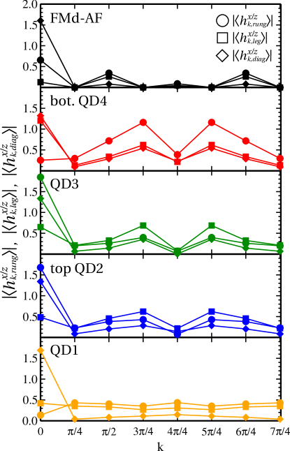
Figure 4: Absolute values of the Fourier transforms of the bond averages $\langle h_{i,{\rm rung}}^{x/z}\rangle$, $\langle h_{i,{\rm leg}}^{x/z}\rangle$, and $\langle h_{i,{\rm diag}}^{x/z}\rangle$, shown in Fig. 3 in the phases FMd-AF, bot. QD4, QD3, top QD2 and QD1. Different symbols — circles, squares, diamonds correspond to rung, leg and diagonal bonds respectively.

The different ground state configurations (phases) realized by the model can be conveniently characterized by a 3D vector field living on one leg of the initial ladder. In three components of such vectors we can encode the average values of three different bonds outgoing from the point at which the vector is anchored — these are leg, rung and diagonal bonds. Because the two legs of the ladder are perfectly equivalent, it is enough to check the following bond operators labeled by a site index $j$ along a single leg, $1\leq j\leq 2L$,

$$h_{j,{\rm rung}}^{x/z}=\begin{cases}X_{i,2}X_{i,3}\equiv\tau_{i,2}^{x}&j=(2i-1)\\ Z_{i,1}Z_{i,4}\equiv\tau_{i,3}^{z}&j=2i\end{cases},$$

$$h_{j,{\rm leg}}^{x/z}=\begin{cases}X_{i,1}X_{i,2}\equiv s_{i}\tau_{i,2}^{x}\tau_{i,3}^{x}&j=(2i-1)\\ Z_{i,1}Z_{i+1,2}\equiv\tau_{i,3}^{z}\tau_{i+1,2}^{z}&j=2i\end{cases},$$

$$h_{j,{\rm diag}}^{x/z}=\begin{cases}X_{i,1}X_{i,3}\equiv s_{i}\tau_{i,3}^{x}&j=(2i-1)\\ Z_{i,1}Z_{i+1,3}\equiv\\ r_{i+1}\tau_{i,3}^{z}\tau_{i+1,2}^{z}\tau_{i+1,3}^{z}&j=2i\end{cases},$$

where $i$ labels the plaquettes, $1\leq i\leq L$. Here we keep in mind that these bonds are of the XX(ZZ) type for odd(even) points along the ladder’s leg. In this way such vector fields tell us all about the NN interactions in a given phase. In this context we can consider a periodicity of a given phase. If the XX and ZZ interactions are perfectly balanced then we can expect that for simplest ground states the bond averages will be the same for every point along the leg and consequently all the vectors will be the same. Such configuration respects the translational and the $r\leftrightarrow s$ interchange symmetry of the initial ladder, as one could expect from the ground state.

To understand better the physical meaning of phases found in the phase diagram of Fig. 2 we present the ground-state values of all different bonds of the initial Hamiltonian shown in Fig. 1. In Fig. 3 we show a 3D representation of the ground-state averages of the above operators as functions of the position $i$ at 15 representative points in the phase diagram. These points are placed in all different phases but also in two pieces of one phase; for instance we have bottom and top part of the FMu phase meaning simply the low- and high-$J_{{\rm rung}}$ parts visible in the phase diagram. This terminology we also apply to few other phases and concerning the FMd phase we write ’wedge’ and ’bubble’ to distinguish between the tiny piece of FMd close to $J_{{\rm leg}}=1.0$ and $J_{{\rm rung}}=J_{{\rm rung}}^{\rm cr}$ and the rest of it.

Figure 2 first shows particular limits, like that: (i) in the nematic phase only the rung bonds are non-zero, or (ii) one has only diagonals or legs non-zero at the compass points, or (iii) the bottom FMu differs from the top FMu phase by the polarization of the rung bonds; in the bottom part the rungs can be neglected but in the top part they are satisfied. Further on, we can see that the wedge part of the FMd phase looks very similar to the compass point from which it stems and in the bubble FMd phase the rung bonds are much more favored. The combined FMdu phase exhibits a strong period $2$ alternation of the bond values whereas in the FMd-AF one the period is $4$. Thus we say that the FMdu phase is dimerized in the sense that going along the ladder we will observe stronger/weaker alternation of a given type of a bond, i.e., leg, rung or diagonal one. Analogously, the FMd-AF is tetramerized. Finally, we find why the QD phases are really disordered as they exhibit no periodicity. This means that translational invariance is completely broken in these phases. Of course, if we average over the degenerate $\left\{r_{i},s_{i}\right\}$ configurations then the translational invariance will be recovered but the system will not gain any energy by forming such a superposition.

Finally, in Fig. 4 we show the Fourier transforms of the bond averages $\langle h_{i,{\rm rung}}^{x/z}\rangle$, $\langle h_{i,{\rm leg}}^{x/z}\rangle$, and $\langle h_{i,{\rm diag}}^{x/z}\rangle$ in the phases with longest periods, namely FMd-AF, bot. QD4, QD3, top QD2 and QD1. These are defined as,

$$\langle h_{k,{\rm bond}}^{x/z}\rangle\equiv\frac{1}{\sqrt{2L}}\sum_{j=1}^{2L}e^{ikj}\langle h_{j,{\rm bond}}^{x/z}\rangle,$$ (25)

with ${\rm bond}={\rm rung},{\rm leg},{\rm diag}$, $k=\frac{2\pi}{2L}n$ and $n=0,1,\dots,2L-1$. In all phases shown in Fig. 4 we see a dominant ferromagnetic order at least for one type of bond meaning large $k=0$ Fourier component. In case of FMd-AF phase we have four non-vanishing Fourier components for any type of bond which indicates a four-site unit cell order. In case of the QD phases all the components are non-vanishing indicating no translational symmetry.

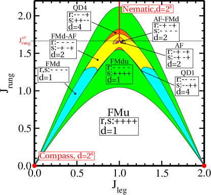
Figure 5: Ground state phase diagram for a system with $L=4$ plaquettes and all $Z$-bonds rescaled by a factor of $\gamma=0.9$ as function of $J_{{\rm leg}}$ and $J_{{\rm rung}}$. The exchange on diagonal bonds $J_{{\rm diag}}$ is set following Eq. (21). The ground states are shaded in color or white and labeled according to their symmetry patterns, $\left\{r_{1},\dots,r_{4},s_{1},\dots,s_{4}\right\}$, which are indicated together with their degeneracies $d$. Red dots are the compass points. The critical value $J_{{\rm rung}}^{{\rm cr}}$ for a nematic state is indicated by horizontal line.

IV.3 A ladder of $L=4$ plaquettes with anisotropic interactions

In the previous Section we studied the phase diagrams of the model given by Eq. (1) with balanced XX and ZZ terms, i.e., they enter with exactly the same exchange interactions. It is interesting to consider as well the present model with unbalanced interactions. In Fig. 5 we show the phase diagram obtained for a ladder of $L=4$ plaquettes in case where all the ZZ interactions are reduced by a factor of $\gamma=0.9$ — of course this does not affect the symmetries that we used so far to get the block-diagonal Hamiltonian. From the point of view of symmetries we loose the $r\leftrightarrow s$ interchange so typically the degeneracies that we find will be reduced by a factor of 2. In the phase diagram we see that first of all the range of stability of FMdu phase is strongly enlarged and that the window between the two pieces of the FMu phase is enlarged too. Now it goes above the classical threshold of $J_{{\rm rung}}=2$ and goes lower at the high symmetry point of $J_{{\rm leg}}=J_{{\rm diag}}=1$.

The enhanced stability of the FMdu phase is clearly due to the fact that the anisotropic interactions brake the symmetry between the $\{r_{i}\}$ and $\{s_{i}\}$ quantum numbers and the FMdu configuration is compatible with such a symmetry breaking. We also notice that the quantum disorder phases are less stable now and two of them are completely absent compared with Fig. 2. On the other hand, we gain two more ordered phases, namely AF-FMd and AF which appear as bubbles instead of bubble FMd phase which is now gone (and the wedge FMd phase is now smaller). This shows clearly that the disordered phases were triggered by frustration caused by the incompatibility of the XX and ZZ interactions. The nematic phase is again unaffected.

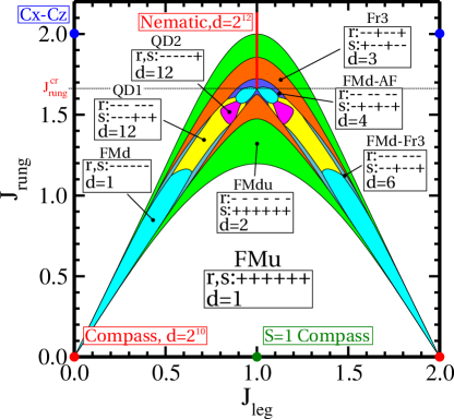
Figure 6: Ground state phase diagram for a ladder consisting of $L=6$ plaquettes as function of $J_{{\rm leg}}$ and $J_{{\rm rung}}$. The exchange on diagonal bonds $J_{{\rm diag}}$ is set following Eq. (21). The ground states are shaded in color or white and labeled according to their symmetry patterns, $\left\{r_{1},\dots,r_{6};s_{1},\dots,s_{6}\right\}$, which are indicated for each phase together with their degeneracies $d$. Red dots are the 1D compass points, blue dots indicate the simple $Cx$–$Cz$ states and green dot is $S=1$ 1D compass point. The critical value $J_{{\rm rung}}^{{\rm cr}}$ for a nematic state is indicated by horizontal line.

V Generic phases for large $L$

V.1 Phase diagram for a ladder of $L=6$ plaquettes

We now increase the system size to identify generic phases in the phase diagram of Fig. 2, and to check which ones could follow from finite-size effects. Figure 6 confirms that several phases we have found for a short ladder of $L=4$ plaquettes reappear for $L=6$. These are FMu, FMd, FMdu and FMd-AF phases. The disordered phases found before are gone but there are others appearing instead. There are also other ordered phases with a longer period $3$, namely Fr3 (ferrimagnetic with period 3) which is stable in a large area of the central region of the window and FMd-Fr3 which replaces former QD1 phase. Period $3$ is now allowed by the system size and we anticipate that it is favorable from the point of view of the three-site terms in the block-diagonal Hamiltonian so we can expect such phases whenever $L$ is divisible by $3$.

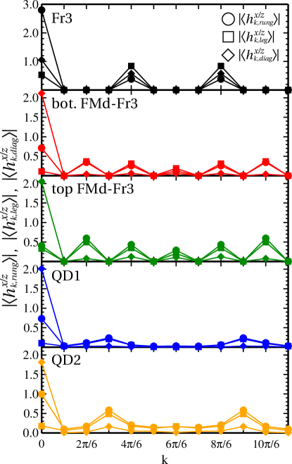
Figure 7: Absolute values of the Fourier transforms of the bond averages $\langle h_{i,{\rm rung}}^{x/z}\rangle$, $\langle h_{i,{\rm leg}}^{x/z}\rangle$, and $\langle h_{i,{\rm diag}}^{x/z}\rangle$, shown in Fig. 8 in the phases FMd-AF, bot. QD4, QD3, top QD2 and QD1. Different symbols - circles, squares, diamonds correspond to rung, leg and diagonal bonds respectively.

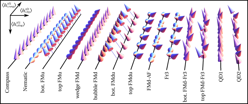
Figure 8: Visualization of the configurations present in the phase diagram of Fig. 6. The solid lines indicate both system itself and different phases or different pieces of one phase which are labeled below. Arrows show the strength of the XX or ZZ interactions within consecutive plaquettes of the systems such that their 3D components correspond to ground-state average of the rung, leg and diagonal interactions denoted as $\langle h_{i,{\rm rung}}^{x/z}\rangle$, $\langle h_{i,{\rm leg}}^{x/z}\rangle$, and $\langle h_{i,{\rm diag}}^{x/z}\rangle$, respectively. The reference frame is given in the left top corner. Arrows along the solid lines mean that only rung interactions are non-zero, vertical arrows mean only diagonal interactions and horizontal ones only along the legs.

Again, we find quantum disordered (QD) phases, this time QD1 and QD2. QD1 phase takes the most of the area where FMd-AF one is stable for $L=4$, whereas the QD2 phase appears in the form of bubbles that stem from the bubbles of FMd phase which are now much larger than for $L=4$. The degeneracy is twice larger in QD2 phase (and also some others) than predicted only by a translation argument, i.e., for a label $\vec{r}=\vec{s}=\left(-----+\right)$ we can generate only five other distinct ground states by a translation by moving simply the $+$ spin, suggesting $d=6$, whereas the degeneracy is de facto $d=12$. Now we can check the action of the $r\leftrightarrow s$ inversion; we take the configuration $\vec{r}=\vec{s}=\left(-----+\right)$ and we get $\vec{r}=\left(+-----\right)$ and $\vec{s}=\left(-----+\right)$ ones. Note that quite counter-intuitively we go from the configuration with $\vec{r}=\vec{s}$ to the one with $\vec{r}\not=\vec{s}$ keeping the energy spectrum unchanged. Then by performing translations once again we can get the other five configurations which explains the total degeneracy of $d=12=2\times(1+5)$. Quite remarkably, all these changes in the phase diagram do not affect the nematic phase which occurs for the same parameters as before.

Figure 7 presents the Fourier transforms of the bond averages $\langle h_{i,{\rm rung}}^{x/z}\rangle$, $\langle h_{i,{\rm leg}}^{x/z}\rangle$, and $\langle h_{i,{\rm diag}}^{x/z}\rangle$ (defined by Eq. 25) in the phases with the longest periods, namely Fr3, bot. FMd-Fr3, QD3, top FMd-Fr3, QD1 and QD2. As for $L=4$ we see that in all phases there is a dominant ferromagnetic component at least for one type of bond meaning large contribution at $k=0$. In case of Fr3 phase we have three non-vanishing Fourier components for any type of bond which indicates a three-site unit cell order. In case of mixed, FMd-Fr3 phases, top and bottom, the number of non-vanishing components is six which corresponds to a six-site unit cell order. As expected in the QD phases all the Fourier components are non-vanishing indicating disorder, however for QD1 most of them are small apart from dominant $k=0$ contribution.

Finally, in Fig. 8 we visualize the bond averages for different phases in the phase diagram of Fig. 6. The phases that were present before (for $L=4$) look here in a similar way as in Fig. 3 so we focus on period-$3$ and disordered phases. We see that indeed phase Fr3 has a periodicity $3$ and every three sites there is a strong increase in diagonal correlations which are weak otherwise and the dominant contribution to the energy comes from the rungs. The mixed FMd-Fr3 phase doubles the period $3$ and favors the diagonals (or legs if $J_{{\rm leg}}>1$). Thus we see that there is a spontaneous trimerization occurring in the phase Fr3 whereas the FMd-Fr3 one is hexamerized. The disordered QD1 phase is very weakly disordered and similar to the wedge FMd phase or the compass one. The disorder in the QD2 phase seems to be stronger than in the QD1 one and is qualitatively similar to the top part of the FMd-Fr3 phase.

V.2 Larger ladder of $L=8$ plaquettes

To check the generality of the phase diagrams shown in previous Sections we explored the cases of larger plaquette ladders, $L=8$ and $L=12$. In Fig. 9 we show the phase diagram for $L=8$. The diagram was obtained in the following way: First the $J_{{\rm leg}}-J_{{\rm rung}}$ parameter plane was discretized as a lattice of $40\times 20$ points and in each point all $4116$ symmetry-distinct $\left\{r_{1},\dots,r_{L};s_{1},\dots,s_{L}\right\}$ subspaces were searched for the ground state and then the subspaces with lowest energy were selected as stable configurations for every lattice point. In this way we identified eight different phases which are realized by the $L=8$-plaquette ladder, shown in Fig. 9. Note that unlike in the previous cases we did not refine the boundaries between the phases by a bisection algorithm but we used a higher-resolution lattice of $100\times 200$ points looking only at these eight subspaces found before. Thus every pixel in the plot of Fig. 9 symbolizes a lattice point with a color determined by the optimal $\left\{r_{1},\dots,r_{L};s_{1},\dots,s_{L}\right\}$ configuration.

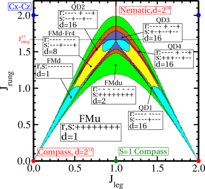
Figure 9: Ground state phase diagram for a ladder consisting of $L=8$ plaquettes as function of $J_{{\rm leg}}$ and $J_{{\rm rung}}$. The exchange on diagonal bonds $J_{{\rm diag}}$ is set following Eq. (21). The ground states are shaded in color or white and labeled according to their symmetry patterns, $\left\{r_{1},\dots,r_{8};s_{1},\dots,s_{8}\right\}$, which are indicated for each phase together with their degeneracies $d$. Red dots are the 1D compass points, blue dots indicate the simple $Cx$–$Cz$ states and green dot is $S=1$ 1D compass point. The critical value $J_{{\rm rung}}^{{\rm cr}}$ for a nematic state is indicated by horizontal line.

Looking at the phase diagram of Fig. 9 we observe an overall similarity to the phase diagrams obtained for $L=4$ and $L=6$ (shown in Figs. 2 and 6), i.e., the number of eight distinct phases is the same as in these two cases. The main difference is the absence of the FMd-AF phase which is here replaced by the FMd-Fr4 one. This can be seen as a generalization of FMd-AF where the period-$2$ AF order is replaced by Fr4 with a period-$4$. As $L=8$ is not a multiplicity of $3$, the phases with period $3$ are absent here and the diagram resembles more the one for $L=4$. Instead of Fr3 phase one finds now two QD phases: QD2 and QD4. We remark that QD2 phase looks quite similar to Fr3 if we analyze the values of $r_{i}$ and $s_{i}$. In addition, FMd-Fr3 phase found before at $L=6$ becomes here QD1 phase for the same reason as above, and again certain similarity between these phases is observed.

In fact, one may also start from a larger $L=8$ system, and one finds that phase FMd-Fr4 is replaced at $L=6$ by two QD phases: QD1 and QD2. These phases arise as a finite size effect but are similar to the original FMd-Fr4 which is incompatible with the length of $L=6$. More generally, we emphasize that the phase FMd-Fr($L/2$) is generic and appears for any length $L=4n$, as demonstrated below by $L=12$ accessible in our analysis. Quite surprisingly, FMd-AF phase found at $L=6$, does not survive for $L=8$ and is there replaced by QD3, cf. Figs. 6 and 9. This suggests that FMd-AF phase is gradually destabilized with increasing size $L$, and indeed it is found only is a very narrow parameter range for $L=12$, see below.

V.3 Largest ladder of $L=12$ plaquettes

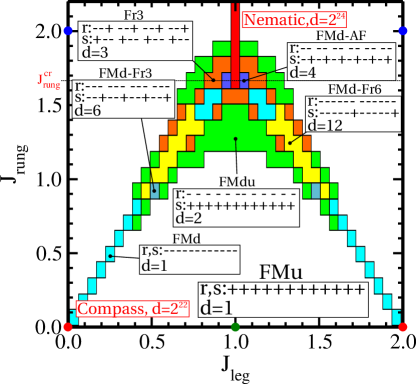
Figure 10: Restricted ground state phase diagram for a ladder consisting of $L=12$ plaquettes as function of $J_{{\rm leg}}$ and $J_{{\rm rung}}$ comparing stability of seven different $\left\{r_{1},\dots,r_{12};s_{1},\dots,s_{12}\right\}$ configurations with degeneracy $d$ indicated by color shading or white. The exchange on diagonal bonds $J_{{\rm diag}}$ is set following Eq. (21). Red dots are the 1D compass points, blue dots indicate the simple $Cx$–$Cz$ states and green dot is $S=1$ 1D compass point. The critical value $J_{{\rm rung}}^{{\rm cr}}$ for a nematic state is indicated by a horizontal line.

Finally we may ask what happens to the phases with period-$2$ and -$4$ in case when also period-$3$ ones are allowed by the system size $L$. This is a case when $L$ is divisible both by $4$ and by $3$ and the lowest possible $L$ satisfying these condition is $L=12$. In Fig. 10 we can see a restricted phase diagram for this case in low resolution. This follows from a lattice of $40\times 20$ points in the $J_{{\rm leg}}-J_{{\rm rung}}$ plane for which we compare the ground state energies of the eight configurations with translational symmetry obtained for lower $L$, namely: FMd, FMu, FMdu, FMd-AF, Fr3, FMd-Fr3, FMd-Fr4, and FMd-Fr6 phase. The latter one is another generalization of FMd-AF phase with a longer period. Indeed, the FMd-Fr6 phase is stable in a region between wedge and bubble FMd phase, see the phase diagram of Fig. 10, and seems to be analogous of the FMd-Fr4 phase found for $L=8$ and FMd-AF one found for $L=4$. Note that the FMd-Fr4 phase is absent here, and the FMd-AF one appears only in two points in the phase diagram close to the onset of the nematic phase. We anticipate that it occurs in place of some QD phase which was not considered here.

Thus we can conclude that for general $L$ divisible by $4$ an FMd-Fr$(L/2)$ phase appears in this part of phase diagram, with $r_{i}\equiv-1$ and with most of $s_{i}=-1$ except for $s_{L/2}=s_{L}=1$. For smaller system sizes a similar phase was less robust. For instance, the phase diagram for $L=6$, see Fig. 6, suggests in this parameter range a QD1-like phase which has similar properties as the FMd-Fr3 one — all $r_{i}\equiv-1$ and almost all $s_{i}=-1$ except for two sites placed irregularly. Concerning the period-3 phases, namely Fr3 and FMd-Fr3, we see that they appear in similar positions as in the $L=6$ phase diagram, so we argue that they are generic for $L$ divisible by $3$. Moreover, it seems that QD phases observed at smaller system sizes appear because ordered characteristic of large $L$ cannot yet develop.

VI Perturbative expansion around nematic phase

The nematic phase is the exact eigenstate of the Hamiltonian and thus it is a good starting point of a perturbative expansion around the high-symmetry line Eq. (14) characterized in Sec. III. For high enough value of $J_{{\rm rung}}$ we start by taking the Hamiltonian in the form of Eq. (9) and dividing it into the unperturbed part ${\cal H}_{0}$ proportional to $J_{{\rm rung}}$ and the rest which will be treated as perturbation, ${\cal V}={\cal H}-{\cal H}_{0}$, we get,

$${\cal H}_{0} = J_{{\rm rung}}\sum_{i=1}^{L}\left(\tau_{i,2}^{x}+\tau_{i,3}^{z}\right),$$ (26)

$${\cal V} = \sum_{i=1}^{L}\left(\tau_{i,2}^{z}{\cal A}_{i}+\tau_{i,3}^{x}{\cal B}_{i}\right),$$ (27)

where,

$${\cal A}_{i} \!\equiv\! J_{{\rm leg}}\!\left(r_{i}\tau_{i,3}^{z}\!+\!\tau_{i-1,3}^{z}\right)\!+\!J_{{\rm diag}}\left(1\!+\!r_{i}\tau_{i-1,3}^{z}\tau_{i,3}^{z}\right)\!,$$ (28)

$${\cal B}_{i} \!\equiv\! J_{{\rm leg}}\!\left(s_{i}\tau_{i,2}^{x}\!+\!\tau_{i+1,2}^{x}\right)\!+\!J_{{\rm diag}}\left(s_{i}\!+\!\tau_{i,2}^{x}\tau_{i+1,2}^{x}\right).$$ (29)

Note that both ${\cal A}_{i}$ and ${\cal B}_{i}$ commute with ${\cal H}_{0}$ so the only terms in ${\cal V}$ that will make the excitations in the eigenstates of ${\cal H}_{0}$ are $\tau_{i,2}^{z}$ and $\tau_{i,3}^{x}$ that play the role of transverse fields. In the zeroth order the ground state is a product state of the form $|\psi_{0}^{(0)}\rangle=\bigotimes_{i}\left|\leftarrow\right\rangle_{i,2}\otimes\left|\downarrow\right\rangle_{i,3}$, and with ground-state energy $E_{0}^{(0)}=-2LJ_{{\rm rung}}$. We remark that for $J_{{\rm leg}}=J_{{\rm diag}}$ and any $r_{i}$ and $s_{i}$ operators ${\cal A}_{i}$ and ${\cal B}_{i}$ annihilate the ground state $|\psi_{0}^{(0)}\rangle$, i.e., ${\cal A}_{i}|\psi_{0}^{(0)}\rangle\equiv{\cal B}_{i}|\psi_{0}^{(0)}\rangle\equiv 0$, so at $J_{{\rm leg}}=J_{{\rm diag}}$ $|\psi_{0}^{(0)}\rangle$ becomes an exact ground state of the full Hamiltonian ${\cal H}$. Using the textbook perturbative expansion we easily find that the first order correction vanishes, i.e., $E_{0}^{(1)}=0$ and the second order correction has a form of,

$$E_{0}^{(2)}=-\frac{(\delta J)^{2}}{J_{{\rm rung}}}\sum_{i=1}^{L}\left(2+r_{i}+s_{i}\right),$$ (30)

with $\delta J\equiv J_{{\rm leg}}-J_{{\rm diag}}$. Note that the correction gives lowest energy for $r_{i}\equiv s_{i}\equiv 1$ which means that for large enough $J_{{\rm rung}}$ close to high symmetry line $\delta J=0$ the optimal configuration (phase) is FMu. This agrees with all the phase diagrams shown in previous Sections. We also easily notice that for fixed $J_{{\rm rung}}$ the energy gap around nematic phases closes as $(\delta J)^{2}$.

Now it is interesting to see what happens in higher orders of the expansion. The next non-vanishing order is the fourth order. Doing the expansion one gets four types of contributions to the fourth order energy correction $E_{0}^{(4)}$ but only one is of the order of $(\delta J)^{2}$ and the rest is of higher orders in $\delta J$. Since we are interested in the neighborhood of the nematic phase, only this lowest order contribution is relevant. We get,

$$E_{0}^{(4)}\!=\!-\frac{(\delta J)^{2}(\sigma J)^{2}}{J_{{\rm rung}}^{3}}\sum_{i=1}^{L}\left(2\!-r_{i}s_{i}\!-r_{i+1}s_{i}\right)+{\cal O}\!\left(\delta J^{3}\right)\!,$$ (31)

with $\sigma J\equiv J_{{\rm leg}}+J_{{\rm diag}}$. This correction contains an AF interaction term between classical spins $r_{i}$ and $s_{i}$ so the optimal configuration for $E_{0}^{(4)}$ is FMdu. We see now that the effective fourth-order Hamiltonian for the classical spins around the nematic phase, namely

$$H_{{\rm eff}}\equiv E_{0}^{(0)}+E_{0}^{(2)}+E_{0}^{(4)},$$ (32)

describes a competition between FMu and FMdu phases. In the upper part of the phase diagram ($J_{\rm rung}>2.0$) FMu phase wins in the large $J_{{\rm rung}}$ limit whereas FMdu phase is stable for lower values of $J_{{\rm rung}}$. We found that the transition point is $J_{{\rm rung}}^{\star}\simeq 1.42$ and that these two phases are the only ones that are stable. The value of $J_{{\rm rung}}^{\star}$ however does not agree with the upper boundary $J_{{\rm rung}}=2$ between FMdu and FMu phases around $\delta J=0$, found in the phase diagrams of Figs. 2, 6, 9, and 10. This shows that the phase competition around the nematic phase in the low $J_{{\rm rung}}$ regime is very complex indeed and requires higher orders of the expansion to resolve the question of stability.

VII Entanglement in the ladders with $L=4$ and $L=6$ plaquettes

VII.1 Dimer-dimer entanglement

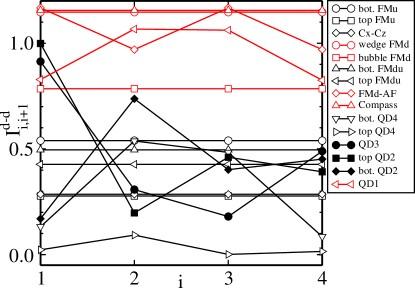
Figure 11: Mutual information $I_{i,i+1}^{d-d}$ (33) between the NN dimers as a function of $i$ for a ladder of $L=4$ plaquettes obtained in different phases and pieces of one phase shown in the phase diagram of Fig. 2. The (top) red lines are for phases in which $I_{i,i+1}^{d-d}$ is on average high ($I\simeq 1$) and the black (bottom) lines are for those in which $I_{i,i+1}^{d-d}$ is on average low ($I\lesssim 0.55$).

To quantify the entanglement of the states described in Figs. 3 and 8 we will evaluate the mutual information $I_{i,i+1}^{d-d}$ of the neighboring dimers (with PBCs) in each of these states as function of the site index $i$. By a dimer we understand pairs of transformed pseudospins $\{\tau_{i,2},\tau_{i,3}\}$ that appear in the block diagonal Hamiltonian of Eq. (1). The mutual information is defined by the von Neumann entropies of the individual dimers $i$ and $i+1$ and the pair of dimers $\left\{i,i+1\right\}$ as follows,

$$I_{i,i+1}^{d-d}=S_{i}^{d}+S_{i+1}^{d}-S_{i,i+1}^{d,d},$$ (33)

where the von Neumann entropy $S_{A}$ of any subsystem $A$ is given by the formula Ami08 ; Tho10 ; Lun12 ,

$$S_{A}=-\mbox{Tr}\rho_{A}\log_{2}\rho_{A},$$ (34)

with $\rho_{A}$ being the reduced density matrix of the subsystem $A$ (i.e., the density matrix $\rho$ of the whole system is traced over all degrees of freedom outside the subsystem $A$). Note that the subsystem $A$ can also stand for a part of degrees of freedom in the entire system as done in the spin-orbital systems You15 . In practice, it is convenient to express $\rho_{A}$ in terms of ground-state correlation functions. For instance $\rho_{i}^{d}$ for a single dimer $i$ can be written as,

$$\rho_{i}^{d}=\frac{1}{2^{2}}\sum_{{\alpha,\beta=\atop 0,x,y,z}}\tau_{i,2}^{\alpha}\tau_{i,3}^{\beta}\left\langle\tau_{i,2}^{\alpha}\tau_{i,3}^{\beta}\right\rangle,$$ (35)

where $\tau_{i,p}^{0}\equiv 1$ and $\tau_{i,p}^{y}\equiv-i\tau_{i,p}^{z}\tau_{i,p}^{x}$ and where the two $\tau$ operators in front of the average live in a local Hilbert space of a single dimer ($\rho_{i}$ is a $4\times 4$ matrix). Similarly, for a pair of dimers we can calculate $\rho_{i,i+1}^{d,d}$ from a formula,

$$\rho_{i,i+1}^{d,d}\!=\!\frac{1}{2^{4}}\!\!\sum_{{\alpha,\beta,\gamma,\delta=\atop 0,x,y,z}}\!\!\tau_{i,2}^{\alpha}\tau_{i,3}^{\beta}\tau_{i+1,2}^{\gamma}\tau_{i+1,3}^{\delta}\!\left\langle\!\tau_{i,2}^{\alpha}\tau_{i,3}^{\beta}\tau_{i+1,2}^{\gamma}\tau_{i+1,3}^{\delta}\!\right\rangle\,.$$ (36)

In Fig. 11 we show the mutual information $I_{i,i+1}^{d-d}$ (33) for the ground states of the ladder of $L=4$ plaquettes shown in Fig. 3 and for ground state at the $Cx$–$Cz$ point as function of $i$. The $Cx$-$Cz$ point is taken to compare the entanglement in the present cases to the one found for the unfrustrated $Cx$–$Cz$ model in Ref. Brz14 which was found to be characterized by $I_{Cx-Cz}=0.28464$. Here we recover this value working in a different basis and we find that typically the phases not obtained before in the unfrustrated case are more entangled. Note that the nematic phase is not shown here because its ground state in terms of operators $\tau_{i}$ is a classical product state and by the definition of Eq. (33) it has a vanishing mutual information.

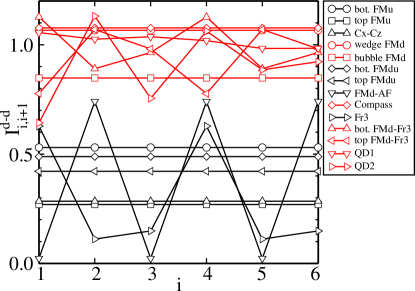
Figure 12: Mutual information $I_{i,i+1}^{d-d}$ (33) between the NN dimers as a function of $i$ for a ladder of $L=6$ plaquettes obtained in different phases and pieces of one phase shown in the phase diagram of Fig. 6. The red (top) lines are for phases in which $I_{i,i+1}^{d-d}$ is on average high ($I\simeq 1$) and the black (bottom) ones are for those in which $I_{i,i+1}^{d-d}$ is on average low ($I\lesssim 0.55$).

In Fig. 11 we marked the phases in which $I_{i,i+1}^{d-d}$ is high ($I\simeq 1.0$) on average and we find that these are both wedge and bubble FMd phases but also FMd-AF and compass ones, together with QD1 phase which is a tiny scrap at the interface of FMd and FMd-AF phases (see Fig. 2). All these phases can be seen as an evolution of the compass phase for finite $J_{{\rm leg}}$ and $J_{{\rm rung}}$ and indeed altogether they connect the two compass points. The entanglement seems to decrease when $J_{{\rm rung}}$ is strongly increased, for instance in the bubble FMd phase. Quite surprisingly the quantum disordered phase apart from QD1 do not seem to be strongly entangled although in QD2 and QD3 phases the mutual information $I_{i,i+1}$ (33) can be enhanced locally to rather high values.

As we can see from Fig. 12, for the larger ladder of $L=6$ plaquettes division between more and less entangled phases seems to be clearer. Again we observe that the phases which can be seen as continuation of the compass points in the phase diagram of Fig. 6 are highly entangled. These are FMd, FMd-AF, QD1, QD2, and FMd-Fr3 phases and the compass states themselves. This suggests that the two compass points are the sources of entanglement in the phase diagram of the extended $Cx$–$Cz$ model, and the phases that are realized are always such that it is possible to move continuously from one point to another keeping the entanglement high. This could be seen as some kind of a conservation law, as if the entanglement played a role of charge here.

Finally, we note that quite counterintuitively at the $S=1$ compass point, i.e., $J_{{\rm rung}}=0$ and $J_{{\rm leg}}=J_{{\rm diag}}$, the dimer-dimer mutual information is not big a for any of these two systems and takes value of $I_{S=1}\simeq 0.45$. Naively one could expect that it should be even higher than at the compass point $J_{{\rm leg}}=0$ because frustration seems to be enhanced by perfectly balanced leg and diagonal bonds. Nevertheless it is smaller and it grows monotonously both when moving horizontally and vertically from the $S=1$ compass point, as long as one stays within the FMu phase.

VII.2 Plaquette-plaquette entanglement

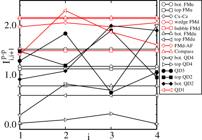
Figure 13: Mutual information $I_{i,i+1}^{p-p}$ (33) between the NN plaquettes as a function of $i$ for a ladder of $L=4$ plaquettes obtained in different phases and pieces of one phase, shown in the phase diagram of Fig. 2. The line colors and characters are the same as in Fig. 11.

Intuitively one expects that the dimer-dimer entanglement described in the previous Subsection should be equivalent to the plaquette-plaquette entanglement of the original ladder shown in Fig. 1. However, this is not so obvious because mutual information is not a basis-independent quantity. The basis dependence comes from taking the partial trace in order to obtain a reduced density matrix. This is why we decide to examine the question of plaquette-plaquette entanglement in the initial, physical basis. Similarly as before we define the mutual information of the NN plaquettes as,

$$I_{i,i+1}^{p-p}=S_{i}^{p}+S_{i+1}^{p}-S_{i,i+1}^{p,p},$$ (37)

where by a plaquette $i$ we understand a subsystem composed of four initial spins $\{X_{i,p},Y_{i,p},Z_{i,p}\}$ with $p=1,2,3,4$. To calculate this quantity we express the relevant reduce density matrices in terms of correlation function as,

$$\rho_{i}^{p}=\frac{1}{2^{4}}\sum_{{A,B,C,D=\atop 1,X,Y,Z}}A_{i,1}B_{i,2}C_{i,3}D_{i,4}\left\langle A_{i,1}B_{i,2}C_{i,3}D_{i,4}\right\rangle,$$ (38)

for a single plaquette and for two plaquettes the expression is analogous but with eight Pauli operators. Our ground state is expressed in terms of spins $\tau_{i,2}$ and $\tau_{i,3}$ so we need to use the transformations of Eqs. (3) and (4). The sum contains $4^{4}$ terms but because of the fixed parities $r_{i}$ and $s_{i}$ only 32 ground-state averages are non-zero. One has to be careful with the signs because operators under average contain $r_{i}^{\star}$ and $s_{i}^{\star}$ which anticommute not only with $r_{i}$ and $s_{i}$ but also with $\tau_{i,3}^{z}$ and $\tau_{i,3}^{x}$. Note that the average will be non-zero only if all $r_{i}^{\star}$ and $s_{i}^{\star}$ appear even number of times to cancel each other since $(r_{i}^{\star})^{2}\equiv(s_{i}^{\star})^{2}\equiv 1$. In case of the reduce density matrix of a pairs of plaquettes the situation is even more complicated. For non-neighboring plaquettes the number of non-vanishing averages is simply $32^{2}$ because these plaquettes can be treated ’independently’. In case of NN plaquettes this number grows to $2\times 32^{2}$.

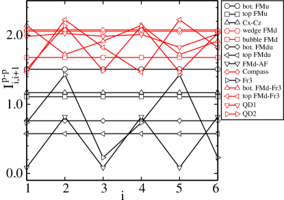
Figure 14: Mutual information $I_{i,i+1}^{p-p}$ (33) between the NN plaquettes as a function of $i$ for a ladder of $L=6$ plaquettes obtained in different phases and pieces of one phase, shown in the phase diagram of Fig. 6. The line colors and characters are the same as in Fig. 11.

In Figs. 13 and 14 we show the results obtained for the mutual information of two NN plaquettes for $L=4$ and $L=6$ for the same points in the phase diagrams as in case of dimers. Note that the vertical scale is twice as large as for pairs of dimers because von Neumann entropy and hence mutual information are extensive quantities. From these plots we can draw analogical conclusions as before because qualitatively they are similar to Figs. 11 and 12. This shows that the entanglement between dimers can be treated as qualitatively equivalent to the entanglement of initial plaquettes. Consequently, the nematic phase exhibits no plaquette-plaquette entanglement.

VIII Summary and conclusions

We have investigated the consequences of frustration in the 1D plaquette compass $Cx$–$Cz$ model with additional frustration due to finite antiferromagnetic exchange on plaquette diagonals. We have used a systematic approach based on the symmetry properties and demonstrated that different possible ground states of this model are characterized by the eigenvalues of the local parity operators being the symmetries of the model. A similar approach was used before for the 2D compass model Brz10 and the 1D plaquette $Cx$–$Cz$ compass model Brz14 , but in these cases the ground state was always found in the simplest possible subspace where all the symmetry eigenvalues (parities) are positive. Here we have seen that due to frustration caused by next nearest neighbor compass interactions along diagonal bonds in the ladder, there is a window in the parameter space $\{J_{\rm leg},J_{\rm rung}\}$ where such a highly symmetric ground state, called here FMu, becomes unstable and one finds instead more exotic phase patterns containing negative parities. Examples of such phases are an anti-FMu configuration, namely FMd where all the parities are negative, or various configurations where the parities alternate. Furthermore, we have shown that some of these states can be stable for arbitrary system size whereas others are strongly related to small system sizes, i.e., ladders of $L=4$ or $L=6$ plaquettes.

We argue that the window of exotic phases stems from the frustration that one already finds for a single plaquette with ZZ interactions only. Especially, the window for perfectly balanced XX and ZZ bonds never goes above $J_{{\rm rung}}=2$, which is a value predicted by a single plaquette study, and its shoulders cover the phase transition lines encountered for a single plaquette. We have shown, however, that it can become broader (exceeding $J_{{\rm rung}}=2$) when the anisotropy between XX and ZZ bonds is introduced. We note that in any case the window of exotic phases in the phase diagram connects two points in the phase diagram where the model is equivalent to the 1D compass model, namely $J_{{\rm rung}}=0$ and $J_{{\rm leg}}=0(2)$, with $J_{{\rm diag}}$ given by Eq. (21). It suggests that these phases are a continuation of the degenerate manifold of ground states of this peculiar 1D model Eri09 ; Liu12 .

One could expect that the ground states always respect the symmetries of the initial ladder: (i) translational ones and (ii) the $r\leftrightarrow s$ interchange invariance. However, we have observed that for ladders of up to $L=12$ plaquettes, the ground states exhibit lower symmetry than that of the initial ladder in the highly frustrated window in the phase diagram, and this manifests itself by ordered states with a longer period, i.e., spontaneous multimerization. In particular, we have obtained four phases that seem to be stable for any even $L$, two of them (FMu and FMd) preserve full translational invariance while one (FMdu) is dimerized and one (FMd-AF) is tetramerized. We note that a similar dimerization due to purely quantum fluctuations was recently found in the Kumar-Heisenberg model gang4 , but in contrast to it here the transition to the dimerized state is discontinuous. In addition, we have found that for a system size $L$ being a multiplicity of three (and even), two other configurations can be stabilized, one with a unit cell of three — Fr3 — and for the cell of six sites — FMd-Fr3. These are examples of trimerized and hexamerized ground states. We argue that the trimmers are compatible with the three-site interactions in the effective Hamiltonian that stem from the diagonal bonds. Apart from these rather regular phases we have also found configurations that we called quantum disordered in the sense that their periodicity was equal to the system length $2L$. These phases were different for $L=4$ and $L=6$, and we suggest that they occur only in so small systems while they are gradually destabilized by ordered phases with longer periods when the system size increases.

Finally, for high enough $J_{{\rm rung}}$, here $J_{{\rm rung}}\geq J_{{\rm rung}}^{{\rm cr}}\simeq 1.664$, and maximal frustration of leg and diagonal interactions, i.e., $J_{{\rm leg}}=J_{{\rm diag}}=1$, we have observed a nematic phase from $L=4$ to $L=12$ and in the anisotropic ladder of $L=4$ plaquettes as well. Nematicity here means that the state is an eigenstate of all rung bonds of the ladder optimizing their energies but in the same time it is an eigenstate with zero energy of the ladder Hamiltonian without rungs. This means that effectively only the rung bonds contribute to the ground-state energy. We note that this state is similar to the nematic state of the 2D compass model Dou05 ; Dor05 . This observation together with the 1D compass points found in the phase diagrams makes us claim that the present ladder model realizes indeed the paradigm of dimensional crossover within the class of compass models.

Quite surprisingly, the vertical onset of the nematic phase is always well within the window of exotic phases, below the classical boarder of $J_{{\rm rung}}=2$ where the window typically closes. In this area of the phase diagram there is clearly a very subtle competition of several energy scales that results in what we call bubble phases being attached to the line of nematic phase. These bubbles seem to be generic as they are present for $L=4$, 6, and 8, as well as in the anisotropic ladder of $L=4$ plaquettes. In absence of anisotropy these are pieces of the FMd phase which is typically stable in the wedges touching the compass points.

The nematic phase is characterized by a macroscopic degeneracy of $d=2^{2L}$ related to the fact that the values of local parity operators do not affect the energy here and there are $2L$ of them. But in contrast to the compass model on the checkerboard lattice Nas12 , the high degeneracy in the nematic phase and at the compass points is not removed by quantum fluctuations. The nematic phase appears as a highly singular part of the plaquette model where the continuum of states is squeezed to one point. By a perturbative expansion around the nematic phase we have demonstrated a competition between FMu and FMdu phases. FMu (FMdu) phase wins in the large (small) $J_{{\rm rung}}$ limit. In all phase diagrams we have identified a special point of 1D $S=1$ compass model which gives a gapped and unique disordered ground state at $J_{\rm rung}=0$ and $J_{\rm diag}=J_{\rm leg}$.

As stated before, we argue that the window of exotic phases connecting the two compass points in the phase diagram is an evolution of the manifold of compass ground states for finite $J_{{\rm rung}}$. Quite remarkably, this evolution seems to preserve the entanglement that manifests itself by a high mutual information of the neighboring dimers in the effective block-diagonal Hamiltonian or, equivalently, high mutual information of the neighboring plaquettes in the original ladder Hamiltonian. The mutual information seems to be the highest at the compass points whereas it is low in the most prolific FMu phase (including the ground state of the $Cx$–$Cz$ model Brz14 ). However, in the window of exotic phases the entanglement is typically high and comparable to the compass points. We argue that this high entanglement originates from high frustration that can be, to some extent, understood in terms of a single-plaquette study.

Summarizing, we would like to emphasize that the results presented for larger systems of $L=8$ and $L=12$ plaquettes provide enough information to anticipate the possible phases for any $L$. We have shown that phases FMd, FMu, FMdu appear always, as well as FMd-Fr($L/2$) for $L$ divisible by 4, while in other cases when $L$ is divisible by 3 phases Fr3 and FMd-Fr3 appear instead, together with a similar QD1 phase. We have observed that quantum disordered phases appear usually when the system size $L$ is not compatible with the actual unit cell of an ordered phase, favored otherwise in a given range of parameters. We suggest that the obtained phase diagram for $L=12$ plaguettes is already quite close to the ultimate phase diagram in the thermodynamic limit. The presented analysis of so complex phase diagrams proves that the model is challenging enough to address the relevant phases by carrying out an extensive density matrix renormalization group study for relatively large system size $L$ at the level of the original ladder Hamiltonian, as probing of all $\{r_{i},s_{i}\}$ configurations is too demanding beyond the system sizes considered here.

Appendix A Different form of the $Cx$–$Cz$ Hamiltonian

For a simple $Cx$–$Cz$ Hamiltonian of Ref. Brz14 we used the following transformation to $\sigma_{i,2/3}^{x/z}$ Pauli operators to get its block-diagonal form,

$$X_{i,1} = r_{i}^{\star},$$

$$X_{i,2} = r_{i}^{\star}s_{i}\sigma_{i,2}^{x}\sigma_{i,3}^{x}\left(\sigma_{i+1,2}^{x}\right),$$

$$X_{i,3} = r_{i}^{\star}s_{i}\sigma_{i,3}^{x}\left(\sigma_{i+1,2}^{x}\right),$$

$$X_{i,4} = r_{i}^{\star}s_{i}\left(\sigma_{i+1,2}^{x}\right),$$ (39)

and

$$Z_{i,1} = s_{i}^{\star}\sigma_{i,3}^{z},$$

$$Z_{i,2} = s_{i-1}^{\star}\left(\sigma_{i-1,3}^{z}\right)\sigma_{i,2}^{z},$$

$$Z_{i,3} = s_{i-1}^{\star}r_{i}\left(\sigma_{i-1,3}^{z}\right)\sigma_{i,2}^{z}\sigma_{i,3}^{z},$$

$$Z_{i,4} = s_{i}^{\star}.$$ (40)

This gives in the $Cx$–$Cz$ Hamiltonian in the linear-cubic form presented in Ref. Brz14 ,

$$\!{\cal H}\left(J_{\rm diag}=0\right)=$$ (41)

$$\!\sum_{i=1}^{L}\left\{\left(J_{\rm leg}\sigma_{i,2}^{z}+J_{\rm rung}\sigma_{i,3}^{z}\right)\!+\!\left(J_{\rm rung}\sigma_{i,2}^{x}+J_{\rm leg}\sigma_{i,3}^{x}\right)\right.$$

$$+ \!\left.J_{\rm leg}r_{i}\sigma_{i-1,3}^{z}\left(\sigma_{i,2}^{z}\sigma_{i,3}^{z}\right)\!+\!J_{\rm leg}s_{i}\left(\sigma_{i,2}^{x}\sigma_{i,3}^{x}\right)\sigma_{i+1,2}^{x}\right\},$$

whereas in terms of present $\tau_{i,2/3}^{x/z}$ operators we get a linear-quadratic form of Eq. (9) which in this limit simplifies to

$$\!\!{\cal H}\left(J_{{\rm diag}}=0\right)\! = \sum_{i=1}^{L}\left\{J_{{\rm rung}}\left(\tau_{i,2}^{x}+\tau_{i,3}^{z}\right)\right.$$ (42)

$$+ \left.J_{{\rm leg}}\left(s_{i}\tau_{i,2}^{x}\tau_{i,3}^{x}+r_{i}\tau_{i,2}^{z}\tau_{i,3}^{z}\right)\right.$$

$$+ \left.J_{{\rm leg}}\left(\tau_{i,3}^{x}\tau_{i+1,2}^{x}+\tau_{i,3}^{z}\tau_{i+1,2}^{z}\right)\right\}\,.$$

Note that the $\tau_{i,2/3}^{x/z}$ Pauli operators are one-to-one related to the $\sigma_{i,2/3}^{x/z}$ ones by the following identities,

$$\tau_{i,3}^{x} = \sigma_{i,3}^{x}\sigma_{i+1,2}^{x},$$

$$\tau_{i,2}^{x} = \sigma_{i,2}^{x},$$

$$\tau_{i,3}^{z} = \sigma_{i,3}^{z},$$

$$\tau_{i,2}^{z} = \sigma_{i,2}^{z}\sigma_{i-1,3}^{z},$$ (43)

and the backward relations are,

$$\sigma_{i,3}^{x} = \tau_{i,3}^{x}\tau_{i+1,2}^{x},$$

$$\sigma_{i,2}^{x} = \tau_{i,2}^{x},$$

$$\sigma_{i,3}^{z} = \tau_{i,3}^{z},$$

$$\sigma_{i,2}^{z} = \tau_{i-1,3}^{z}\tau_{i,2}^{z}.$$ (44)

References

- (1) L. Amico, R. Fazio, A. Osterloh, and V. Vedral, Rev. Mod. Phys. 80, 517 (2008).
- (2) Bruce Normand, Cont. Phys. 50, 533 (2009).
- (3) Leon Balents, Nature (London) 464, 199 (2010).
- (4) J. Villain, J. Phys. C: Solid State Phys. 10, 1717 (1977).
- (5) L. Longa and A. M. Oleś, J. Phys. A: Math. Theor. 13, 1031 (1980).
- (6) Z. Nussinov and J. van den Brink, Rev. Mod. Phys. 87, 1 (2015).
- (7) S. Wenzel and W. Janke, Phys. Rev. B 78, 064402 (2008).
- (8) H.-D. Chen, C. Fang, J. Hu, and H. Yao, Phys. Rev. B 75, 144401 (2007).
- (9) R. Orús, A. C. Doherty, and G. Vidal, Phys. Rev. Lett. 102, 077203 (2009).
- (10) L. Cincio, J. Dziarmaga, and A. M. Oleś, Phys. Rev. B 82, 104416 (2010).
- (11) P. Czarnik and J. Dziarmaga, Phys. Rev. B 92, 035152 (2015); P. Czarnik, J. Dziarmaga, and A. M. Oleś, ibid. 93, 1844XX (2016).
- (12) W.-L. You, G.-S. Tian, and H.-Q. Liu, J. Phys.: Math. Theor. 43, 275001 (2010).
- (13) W. Brzezicki and A. M. Oleś, Phys. Rev. B 82, 060401(R) (2010); 87, 214421 (2013).
- (14) Z. Nussinov and E. Fradkin, Phys. Rev. B 71, 195120 (2005).
- (15) A. Kitaev, Annals of Physics 303, 2 (2003).
- (16) B. Douçot, M. V. Feigel’man, L. B. Ioffe, and A. S. Ioselevich, Phys. Rev. B 71, 024505 (2005).
- (17) J. Dorier, F. Becca, and F. Mila, Phys. Rev. B 72, 024448 (2005).
- (18) J. Vidal, R. Thomale, K. P. Schmidt, and S. Dusuel, Phys. Rev. B 80, 081104 (2009).
- (19) F. Trousselet, A. M. Oleś, and P. Horsch, Europhys. Lett. 91, 40005 (2010); Phys. Rev. B 86, 134412 (2012).
- (20) A. A. Vladimirov, D. Ihle, and N. Plakida, Eur. Phys. J. B 88, 148 (2015).
- (21) J. Nasu, S. Todo, and S. Ishihara, Phys. Rev. B 85, 205141 (2012); J. Nasu and S. Ishihara, J. Phys.: Conf. Series 320, 012062 (2011).
- (22) K. I. Kugel and D. I. Khomskii, JETP 37, 725 (1973); Usp. Fiz. Nauk 136, 621 (1982) [Sov. Phys. Usp. 25, 231 (1982)].
- (23) L. F. Feiner, A. M. Oleś, and J. Zaanen, Phys. Rev. Lett. 78, 2799 (1997); J. Phys.: Condens. Matter 10, L555 (1998).
- (24) J. van den Brink, Z. Nussinov, and A. M. Oleś, in: Introduction to Frustrated Magnetism: Materials, Experiments, Theory, edited by C. Lacroix, P. Mendels, and F. Mila (Springer, New York, 2011).
- (25) Y. Tokura and N. Nagaosa, Science 288, 462 (2000).
- (26) G. Khaliullin, P. Horsch, and A.M. Oleś, Phys. Rev. Lett. 86, 3879 (2001); Phys. Rev. B 70, 195103 (2004).
- (27) F. Vernay, K. Penc, P. Fazekas, and F. Mila, Phys. Rev. B 70, 014428 (2004); A. Reitsma, L. F. Feiner, and A. M. Oleś, New J. Phys. 7, 121 (2005).
- (28) A. M. Oleś, G. Khaliullin, P. Horsch, and L. F. Feiner, Phys. Rev. B 72, 214431 (2005).
- (29) G. Khaliullin, Prog. Theor. Phys. Suppl. 160, 155 (2005).
- (30) C. Ulrich, A. Gössling, M. Grüninger, M. Guennou, H. Roth, M. Cwik, T. Lorenz, G. Khaliullin, and B. Keimer, Phys. Rev. Lett. 97, 157401 (2006); C. Ulrich, G. Khaliullin, M. Guennou, H. Roth, T. Lorenz, and B. Keimer, ibid. 115, 156403 (2015).
- (31) J. Fujioka, T. Yasue, S. Miyasaka, Y. Yamasaki, T. Arima, H. Sagayama, T. Inami, K. Ishii, and Y. Tokura, Phys. Rev. B 82, 144425 (2010); P. Horsch, A. M. Oleś, L. F. Feiner, and G. Khaliullin, Phys. Rev. Lett. 100, 167205 (2008).
- (32) F. Krüger, S. Kumar, J. Zaanen, and J. van den Brink, Phys. Rev. B 79, 054504 (2009).
- (33) P. Corboz, M. Lajkó, A. M. Laüchli, K. Penc, and F. Mila, Phys. Rev. X 2, 041013 (2012).
- (34) K. Wohlfeld, M. Daghofer, S. Nishimoto, G. Khaliullin, and J. van den Brink, Phys. Rev. Lett. 107, 147201 (2011); P. Marra, K. Wohlfeld, and J. van den Brink, ibid. 109, 117401 (2012); V. Bisogni, K. Wohlfeld, S. Nishimoto, C. Monney, J. Trinckauf, K. Zhou, R. Kraus, K. Koepernik, C. Sekar, V. Strocov, B. Büchner, T. Schmitt, J. van den Brink, and J. Geck, ibid. 114, 096402 (2015); E. M. Plotnikova, M. Daghofer, J. van den Brink, and K. Wohlfeld, ibid. 115, 106401 (2016); K. Wohlfeld, S. Nishimoto, M. W. Haverkort, and J. van den Brink, Phys. Rev. B 88, 195138 (2013); C.-C. Chen, M. van Veenendaal, T. P. Devereaux, and K. Wohlfeld, ibid. 91, 165102 (2015).
- (35) A. M. Oleś, J. Phys.: Condens. Matter 24, 313201 (2012); Acta Phys. Polon. A 127, 163 (2015).
- (36) W. Brzezicki, J. Dziarmaga, and A. M. Oleś, Phys. Rev. Lett. 109, 237201 (2012); Phys. Rev. B 87, 064407 (2013).
- (37) P. Czarnik and J. Dziarmaga, Phys. Rev. B 91, 045101 (2015).
- (38) J. Fujioka, S. Miyasaka, and Y. Tokura, Phys. Rev. B 77, 144402 (2008); P. Horsch and A. M. Oleś, ibid. 84, 064429 (2011); A. Avella, P. Horsch, and A. M. Oleś, ibid. 87, 045132 (2013); A. Avella, A. M. Oleś, and P. Horsch, Phys. Rev. Lett. 115, 206403 (2015).
- (39) W. Brzezicki, A. M. Oleś, and M. Cuoco, Phys. Rev. X 5, 011037 (2015); W. Brzezicki, M. Cuoco, and A. M. Oleś, J. Supercond. Novel Magn. 29, 563 (2016).
- (40) G. Jackeli and G. Khaliullin, Phys. Rev. Lett. 102, 017205 (2009); J. Chaloupka, G. Jackeli, and G. Khaliullin, ibid. 105, 027204 (2010); 110, 097204 (2013); F. Trousselet, M. Berciu, A. M. Oleś, and P. Horsch, ibid. 111, 037205 (2013); J. Chaloupka and G. Khaliullin, Phys. Rev. B 92, 024413 (2015).
- (41) G. Jackeli and A. Avella, Phys. Rev. B 92, 184416 (2015).
- (42) A. Kitaev, Annals of Physics 321, 2 (2006).
- (43) G. Baskaran, S. Mandal, and R. Shankar, Phys. Rev. Lett. 98, 247201 (2007).
- (44) P. Milman, W. Maineult, S. Guibal, L. Guidoni, B. Douçot, L. Ioffe, and T. Coudreau, Phys. Rev. Lett. 99, 020503 (2007).
- (45) A. M. Oleś, P. Horsch, L. F. Feiner, and G. Khaliullin, Phys. Rev. Lett. 96, 147205 (2006); W.-L. You, A. M. Oleś, and P. Horsch, New J. Phys. 17, 083009 (2015); W.-L. You, P. Horsch, and A. M. Oleś, Phys. Rev. B 92, 054423 (2015).
- (46) J. van den Brink, P. Horsch, F. Mack, and A. M. Oleś, Phys. Rev. B 59, 6795 (1999).
- (47) J. van den Brink, New J. Phys. 6, 201 (2004).
- (48) L. F. Feiner and A. M. Oleś, Phys. Rev. B 71, 144422 (2005).
- (49) T. Tanaka, M. Matsumoto, and S. Ishihara, Phys. Rev. Lett. 95, 267204 (2005); T. Tanaka and S. Ishihara, Phys. Rev. Lett. 98, 256402 (2007). .
- (50) M. Daghofer, K. Wohlfeld, A. M. Oleś, E. Arrigoni, P. Horsch, Phys. Rev. Lett. 100, 066403 (2008); K. Wohlfeld, M. Daghofer, A. M. Oleś, P. Horsch, Phys. Rev. B 78, 214423 (2008).
- (51) A. van Rynbach, S. Todo, and S. Trebst, Phys. Rev. Lett. 105, 146402 (2010).
- (52) P. Wróbel and A. M. Oleś, Phys. Rev. Lett. 104, 206401 (2010); P. Wróbel, R. Eder, and A. M. Oleś, Phys. Rev. B 86, 064415 (2012).
- (53) M. Daghofer, A. Nicholson, A. Moreo, and E. Dagotto, Phys. Rev. B 81, 014511 (2010); A. Nicholson, W. Ge, X. Zhang, J. Riera, M. Daghofer, A. M. Oleś, G. B. Martins, A. Moreo, and E. Dagotto, Phys. Rev. Lett. 106, 217002 (2011).
- (54) F. Trousselet, A. Ralko, and A. M. Oleś, Phys. Rev. B 86, 014432 (2012).
- (55) G. Chen and L. Balents, Phys. Rev. Lett. 110, 206401 (2013).
- (56) S. Wenzel and A. M. Läuchli, Phys. Rev. Lett. 106, 197201 (2011).
- (57) W. Brzezicki, J. Dziarmaga, and A. M. Oleś, Phys. Rev. B 75, 134415 (2007); W. Brzezicki and A. M. Oleś, Acta Phys. Polon. A 115, 162 (2009).
- (58) K.-W. Sun, Yu-Yu Zhang, and Q.-H. Chen, Phys. Rev. B 79, 104429 (2009).
- (59) E. Eriksson and H. Johannesson, Phys. Rev. B 79, 224424 (2009).
- (60) G.-H. Liu, W. Li, W.-L. You, G.-S. Tian, and G. Su, Phys. Rev. B 85, 184422 (2012); G.-H. Liu, W. Li, and W.-L. You, Eur. Phys. J. B 85, 168 (2012).
- (61) H. T. Wang and S. Y. Cho, J. Phys.: Condens. Matter 27, 015603 (2015).
- (62) R. Jafari, Phys. Rev. B 84, 035112 (2011).
- (63) W.-L. You, P. Horsch, and A. M. Oleś, Phys. Rev. B 89, 104425 (2014); W.-L. You, G.-H. Liu, P. Horsch, and A. M. Oleś, ibid. 90, 094413 (2014).
- (64) W. Brzezicki and A. M. Oleś, Phys. Rev. B 80, 014405 (2009).
- (65) W. Brzezicki and A. M. Oleś, Phys. Rev. B 90, 024433 (2014).
- (66) S. Wenzel and W. Janke, Phys. Rev. B 80, 054403 (2009).
- (67) M. Biskup and R. Kotecký, J. Stat. Mech.: Theory and Experiment P11001 (2010).
- (68) B. Kumar, Phys. Rev. B 87, 195105 (2013); W. Brzezicki, J. Dziarmaga, and A. M. Oleś, Phys. Rev. Lett. 112, 117204 (2014).
- (69) G.-H. Liu, L.-J. Kong, and W.-L. You, Eur. Phys. J. B 88, 284 (2015).
- (70) R. Thomale, D. P. Arovas, and B. A. Bernevig, Phys. Rev. Lett. 105, 116805 (2010).
- (71) R. Lundgren, V. Chua, and G. A. Fiete, Phys. Rev. B 86, 224422 (2012).
- (72) W.-L. You, A. M. Oleś, and P. Horsch, New J. Phys. 17, 083009 (2015); Phys. Rev. B 86, 094412 (2012); W.-L. You, P. Horsch, and A. M. Oleś, ibid. 92, 054423 (2015).
- (73) W. Brzezicki, I. Hagymási, J. Dziarmaga, and Ö. Legeza, Phys. Rev. B 91, 205137 (2015).