Adiabatic Persistent Contrastive Divergence Learning

Abstract

This paper studies the problem of parameter learning in probabilistic graphical models having latent variables, where the standard approach is the expectation maximization algorithm alternating expectation (E) and maximization (M) steps. However, both E and M steps are computationally intractable for high dimensional data, while the substitution of one step to a faster surrogate for combating against intractability can often cause failure in convergence. We propose a new learning algorithm which is computationally efficient and provably ensures convergence to a correct optimum from the multi-time-scale stochastic approximation theory. Its key idea is to run only a few cycles of Markov Chains (MC) in both E and M steps. Such an idea of running ‘incomplete’ MC has been well studied only for M step in the literature, called Contrastive Divergence (CD) learning. While such known CD-based schemes find approximated solutions via the mean-field approach in E step, our proposed algorithm does exact ones via MC algorithms in both steps. Consequently, the former maximizes an approximation (or lower bound) of log-likelihood, while the latter does the actual one. Despite of the theoretical understandings, the proposed scheme might suffer from the slow mixing of MC in E step. To address the issue, we also propose a hybrid approach adapting both mean-field and MC approximations in E step, and it outperforms the bare mean-field CD schemes in our experiments on real-world datasets.

1 Introduction

Graphical model (GM) has been one of powerful paradigms for succinct representations of joint probability distributions in various scientific fields including information theory, statistical physics and artificial intelligence. GM represents a joint distribution of some random variables by a graph structured model where each vertex corresponds to a random variable and each edge captures the conditional dependence between random variables. We study the problem of learning parameters in graphical models having latent (or hidden) variables. To this end, a standard learning procedure is the expectation maximization (EM) algorithm alternating expectation (E) and maximization (M) steps, where both involve certain inference tasks. However, they are computationally intractable for high-dimensional data.

To address the issue, Hinton et al. [1, 2] suggested the so-called (persistent and non-persistent) Contrastive Divergence (CD) learning algorithms based on the stochastic approximation and mean-field theories. They apply the mean-field approach in E step, and run an incomplete Markov chain (MC) only few cycles in M step, instead of running the chain until it converges or mixes. Consequently, the persistent CD maximizes (a variational lower bound of) the log-likelihood, and the non-persistent CD minimizes the reconstruction error induced by a few cycles of MC. The authors also have demonstrated their performances in deep GMs such as Restricted Boltzmann Machine (RBM) [3] and Deep Boltzmann Machine (DBM) [4] for various applications, e.g., image [5], speech [6] and recommendation [7]. In principle, they are applicable for any GMs with latent variables.

In this paper, we propose a new CD algorithm, called Adiabatic Persistent Contrastive Divergence (APCD). The design principle can be understood as a ‘probabilistic’ analogue of the standard adiabatic theorem [8] in quantum mechanics which states that if a system changes in a reversible manner at an infinitesimally small rate, then it always remains in its ground state. It is computationally efficient and provably ensures convergence to a correct optimum of the log-likelihood. While the persistent mean-field CD maximizes a variational lower bound of the log-likelihood, the proposed algorithm does the actual log-likelihood directly. Our key idea is conceptually simple: run the exact MC method, instead of the mean-field approximation, in E step as well. Namely, APCD runs incomplete MCs in both E and M steps simultaneously. We prove that it converges to a local optimum (or stationary point) of the actual log-likelihood under mild assumptions by extending a standard stochastic approximation theory [9] to the one with multi-time-scales. Such guarantee is hard to obtain under the known mean-field CD learning since it optimizes a biased log-likelihood due to the mean-field errors.

Despite the theoretical understandings, APCD might perform worse in practice than the mean-field CD schemes since E step might take long time to converge, i.e., slow mixing. To address the issue, we also design a hybrid scheme that utilizes both the mean-field and MC advantages in E step. Our experiments on real-world image datasets demonstrate that APCD outperforms the bare mean-field CD scheme under deep GMs. To our best knowledge, APCD is the first efficient algorithm with provable convergence to a correct (local) optimum of log-likelihood for general GMs. We anticipate that applications of our new technique will be of interest to various fields where GMs with latent variables are used for statistical modeling, while some existing deep learning methods, which often perform similarly as APCD in our experiments, were designed for more special purposes without theoretical justifications.

There have been theoretical efforts to understand the CD learning in the literature [10, 11, 12, 13, 14] under the stochastic approximation theory. However, they assume that either E or M step is computable exactly, while APCD runs incomplete MCs in both steps simultaneously. Consequently, analyzing APCD becomes much more challenging since some change in one step to a biased direction can steer the other step towards a wrong direction. The main contribution of our work is to overcome this technical challenge by adopting the multi-time-scale stochastic approximation theory. We adjust learning rates so that one of E and M steps runs in a faster time-scale than the other, leading both steps to have correct estimations of the gradient of log-likelihood.

There have also been several efforts to accelerate the CD schemes via alleviating the slow mixing issue in M step. One of the most popular techniques to boost mixing is simulated tempering [15] which has also been studied in deep GMs recently [16, 17, 18, 19]. The idea is to run a MC with a slowly decreasing temperature under the intuition that the high-temperature distributions are more spread out and easier to sample from than the target distribution. These techniques can also be applicable to the proposed APCD and hence are orthogonal to our work.

2 Preliminaries

2.1 Graphical model

Exponential family. The exponential family is of our interest, defined as follows. We first let $\phi=(\phi_{\alpha}:\alpha\in\mathcal{I})$ be a collection of real-valued functions $\phi_{\alpha}:\mathcal{X}\rightarrow\mathbb{R}$ called potential functions (or simply potentials) or sufficient statistics, where $\mathcal{X}\subset\mathbb{R}^{k}$ is the set of configurations. We assume that $\mathcal{X}$ is a finite set and $\phi$ is bounded. For a given vector of sufficient statistics $\phi$, let $\theta=(\theta_{\alpha}:\alpha\in\mathcal{I})$ be an associated vector called canonical or exponential parameters. For each fixed $x\in\mathcal{X}$, we use $\langle\theta,\phi(x)\rangle$ to denote the inner product of two vectors $\theta$ and $\phi(x)$, i.e., $\langle\theta,\phi(x)\rangle=\sum_{\alpha\in\mathcal{I}}\theta_{\alpha}\phi_{\alpha}(x)$. Using this notation, the exponential family associated with the set of potentials $\phi$ consists of the following collection of density functions:

$$p_{\theta}(x)=\exp\{\langle\theta,\phi(x)\rangle-A(\theta)\},\qquad\mbox{where}\quad A(\theta)=\log\sum_{x\in\mathcal{X}}\exp\langle\theta,\phi(x)\rangle.$$ (1)

Here, $\exp\{A(\theta)\}$ is the normalizing constant called partition function. For a fixed potential vector $\phi$, each parameter vector $\theta$ indexes a particular member $p_{\theta}$ of the family. The canonical parameters $\theta$ of interest belong to the set $\Theta\mathrel{:=}\{\theta\in\mathbb{R}^{|\mathcal{I}|}|A(\theta)<+\infty\}.$

We assume regularity and minimality for the exponential family throughout this paper, i.e., $\Theta$ is an open set and potential functions $(\phi_{\alpha}:\alpha\in\mathcal{I})$ are linearly independent. For any regular exponential family, one can obviously check that $A(\cdot)$ is a smooth and convex function of $\theta$, implying that $\Theta$ must be a convex set. The minimality condition ensures that there exists a unique parameter vector $\theta$ associated with each density in the family.

Mean parameter. It turns out that any exponential family also allows an alternative parameterization by so-called mean parameter $\mu=(\mu_{\alpha}:\alpha\in\mathcal{I})$. For any given density function $p_{\theta}$, the mean parameter $\mu$ associated with a sufficient statistic $\phi$ is defined by the following expectation:

$$\mu_{\alpha}=\mathbb{E}_{\theta}[\phi_{\alpha}(X)]=\sum_{x\in\mathcal{X}}\phi_{\alpha}(x)p_{\theta}(x),\qquad\mbox{for $\alpha\in\mathcal{I},$}$$ (2)

where we also define $\mathcal{M}_{\phi}\mathrel{:=}\left\{\mu\in\mathbb{R}^{|\mathcal{I}|}~{}\Big{|}~{}\exists\,p_{\theta}\ \text{such that}\ \mu=\sum_{x\in\mathcal{X}}\phi(x)p_{\theta}(x)\right\},$ i.e., $\mathcal{M}_{\phi}$ is the set of all realizable mean parameters associated with the given sufficient statistics $\phi.$

The gradient of the log partition function $A(\theta)$ has the following connection to mean parameters:

$$\frac{\partial A(\theta)}{\partial\theta_{\alpha}} = \mathbb{E}_{\theta}[\phi_{\alpha}(X)],\qquad\mbox{for $\alpha\in\mathcal{I},$}$$ (3)

and therefore $\nabla A(\theta)=\mu$, i.e., the mean parameters of $p_{\theta}$. This can be viewed as a forward mapping from $\theta$ to $\mu$. One can easily check that $\nabla A:\Theta\mapsto\mathcal{M}^{\circ}$ for any regular and minimal exponential family is a bijection mapping. Moreover, we denote by $\theta^{*}:\mathcal{M}^{\circ}\mapsto\Theta$ the inverse map of $\nabla A$, i.e., $\theta^{*}(\mu)\mathrel{:=}\nabla A^{-1}(\theta)$, thus $\mu=\mathbb{E}_{\theta^{*}(\mu)}[\phi(X)]$. The existence and the differentiability of $\theta^{*}$ is a direct consequence of the implicit function theorem.

2.2 Expectation maximization

Learning exponential family. For a given potential vector $\phi,$ the goal is to learn exponential parameters $\theta$ given $N$ observed data $\mathbf{x}\mathrel{:=}\{x^{n}:n=1,\dots,N\}$, for which the popular Maximum Likelihood Estimation (MLE) is used by solving the following optimization problem:

$$\text{{\bf MLE:}}\quad\theta^{*}=\text{arg}\max_{\theta\in\Theta}l(\theta;\mathbf{x}),\quad\text{where}\quad l(\theta;\mathbf{x})\mathrel{:=}\frac{1}{N}\sum_{n=1}^{N}\log p_{\theta}(x^{n}).$$

When computing the optimal solution $\theta^{*},$ the gradient of the log-likelihood $l(\theta;\mathbf{x})$ has the following form due to (1) and (3):

$$\frac{\partial l(\theta;\mathbf{x})}{\partial\theta}=\hat{\mu}-\mathbb{E}_{\theta}[\phi(X)],\qquad\text{where}\quad\hat{\mu}\mathrel{:=}\frac{1}{N}\sum_{n=1}^{N}\phi(x^{n}).$$ (4)

Here, $\hat{\mu}$ is called empirical mean parameter. In many applications of graphical models, a configuration $x\in\mathbb{R}^{k}$ tends to have a high dimension, often partially observed, thus some units (i.e., coordinates) of $x$ are hidden (or latent). Thus, we denote by $x=(v,h),\ v\in\mathcal{X}^{v},h\in\mathcal{X}^{h}$ the entire configuration with visible $v$ and hidden $h$ configurations, where $\mathcal{X}^{v}$ and $\mathcal{X}^{h}$ are the domains of visible and hidden ones, respectively. Clearly, $\mathcal{X}=\mathcal{X}^{v}\times\mathcal{X}^{h}.$ Then, the probability density function of the exponential family can be rewritten as $p_{\theta}(v,h)=\exp\{\langle\theta,\phi(v,h)\rangle-A(\theta)\}$, and denote by $p_{\theta}(v)$ the density of a visible configuration $v$ marginalized over hidden units, i.e., $p_{\theta}(v)=\sum_{h\in\mathcal{X}^{h}}p_{\theta}(v,h).$ In presence of hidden units, for $N$ visible data $\mathbf{v}=\{v^{n}:n=1,\dots,N\},$ one aims at still learning parameters using the maximum likelihood principle on marginal log-likelihood $l(\theta;\mathbf{v})$:

$$\text{{\bf MMLE:}}\quad\theta^{*}=\text{arg}\max_{\theta\in\Theta}l(\theta;\mathbf{v}),\quad\text{where}\quad l(\theta;\mathbf{v})=\frac{1}{N}\sum_{n=1}^{N}\log p_{\theta}(v^{n}).$$ (5)

Expectation Maximization. A popular approach solving MMLE is the Expectation Maximization (EM) algorithm. Consider a distribution $q=\{q^{n}(h):n=1,\dots,N\}$ over hidden units of each visible data. Using Jensen’s inequality, a lower bound of $l(\theta;\mathbf{v})$ is given by:

$$l(\theta;\mathbf{v}) =\frac{1}{N}\sum_{n=1}^{N}\log\sum_{h\in\mathcal{X}^{h}}q^{n}(h)\frac{p_{\theta}(v^{n},h)}{q^{n}(h)}\geq\frac{1}{N}\sum_{n=1}^{N}\sum_{h\in\mathcal{X}^{h}}q^{n}(h)\log\frac{p_{\theta}(v^{n},h)}{q^{n}(h)}$$ (6)

$$=\mathcal{F}(q,\theta)\mathrel{:=}\frac{1}{N}\sum_{n=1}^{N}\Big{(}\sum_{h\in\mathcal{X}^{h}}q^{n}(h)\log p_{\theta}(v^{n},h)+H(q^{n})\Big{)},$$ (7)

where $H(q)=-\sum_{h\in\mathcal{X}^{h}}q(h)\log q(h)$ is the entropy of $q$. The EM algorithm, consisting of E and M steps, alternates between maximizing the lower bound $\mathcal{F}(q,\theta)$ with respect to $q$ and $\theta$, respectively, holding the other fixed: at each $t$-th iteration,

$$\text{{\bf E step:}}\quad q_{(t+1)}=\text{arg}\max_{q}\mathcal{F}(q,\theta_{(t)})\quad\quad\text{{\bf M step:}}\quad\theta_{(t+1)}=\text{arg}\max_{\theta}\mathcal{F}(q_{(t+1)},\theta).$$

E step reduces to inferring the probability of hidden units for each given observed data, and it is well known that for exponential family (1), the exact bound holds when $q_{(t+1)}^{n}(h)=p_{\theta_{(t)}}(h|v^{n})$ for each visible data $v^{n}$. Then, we compute the expectation of $\phi(v^{n},H)$, denoted by $\hat{\mu}^{n}_{(t+1)},$ where the random variable $H$ for a hidden configuration has the density $p_{\theta_{(t)}}(h|v^{n})$, and derive the empirical mean parameter $\hat{\mu}$ (as in (4)), which is used in M step, i.e.,

$$\hat{\mu}^{n}_{(t+1)}\mathrel{:=}\sum_{h\in\mathcal{X}^{h}}\phi(v^{n},h)p_{\theta_{(t)}}(h|v^{n}).$$

M step now becomes equal to finding the canonical parameter in MLE (i.e., (4)), which is due to the fact that the entropy of $q$ does not depend on $\theta$ in (6).

Both E and M steps are computationally intractable in general. First, E step requires deducing probability distribution over hidden units from given canonical parameters, and exact inference requires exponential time with respect to the number of hidden units. A similar computational issue also arises in M step. The main contribution of this paper is to develop a computationally efficient learning algorithm that provably converges to a stationary point or local optimum of MMLE.

3 Adiabatic persistent contrastive divergence

Now we are ready to present our main results: an algorithm to learn exponential parameters $\theta$ for a given $\mathbf{v}$ and a graph structure, and the theoretical analysis of the algorithm’s convergence. We first describe the algorithm and then show its provable convergence guarantee.

3.1 Algorithm description

Algorithm 1 Adiabatic Persistent Contrastive Divergence (APCD): At each iteration $t=0,1,\ldots,$

  Input: Visible data $\mathbf{v}=\{v^{n}:n=1,\dots,N\}$,           $M$: the number of MCs, $\ell$: the number of MC transitions to obtain a MC sample.

  Output: Canonical parameter $\theta_{(t)}$.

  Initialize: Set $\theta_{(0)}\in\Theta$, and $\{\hat{h}_{(0)}^{n,m},\hat{x}_{(0)}^{m},\hat{\mu}^{n}_{(0)}:n=1,\dots,N,m=1,\dots,M\}$ arbitrarily.

    

  /* E step */

  for $n=1$ to $N$  do

     for $m=1$ to $M$ do

        E.1. Obtain a random sample $\hat{h}_{(t+1)}^{n,m}$ given $\hat{h}_{(t)}^{n,m}$ by taking $\ell$ transitions of a time-reversible transition matrix $K^{E}_{\theta_{(t)},v^{n}}$ with the invariant distribution $p_{\theta_{(t)}}(h|v^{n}).$ Formally,

$$p_{\theta_{(t)}}(h|v^{n})=p_{\theta_{(t)}}(h|v^{n})K^{E}_{\theta_{(t)},v^{n}}\quad\text{and}\quad\Pr\left[\hat{h}_{(t+1)}^{n,m}=h\mid\hat{h}_{(t)}^{n,m}\right]=(K^{E}_{\theta_{(t)},v^{n}})^{\ell}\big{(}\hat{h}_{(t)}^{n,m},h\big{)}.$$

     end for

     E.2. Update per-data empirical mean parameter $\hat{\mu}_{(t+1)}^{n}$ with the step-size $a_{(t)}$:

$$\hat{\mu}_{(t+1)}^{n} = \hat{\mu}_{(t)}^{n}+a_{(t)}\left(\frac{1}{M}\sum_{m=1}^{M}\phi\Big{(}v^{n},\hat{h}_{(t+1)}^{n,m}\Big{)}-\hat{\mu}_{(t)}^{n}\right).$$ (8)

  end for

  E.3. Update the empirical mean parameter as: $\hat{\mu}_{(t+1)}=\frac{1}{N}\sum_{n=1}^{N}\hat{\mu}_{(t+1)}^{n}.$

  /* M step */

  for $m=1$ to $M$  do

     M.1. Obtain a random sample $\hat{x}_{(t+1)}^{m}$ given $\hat{x}_{(t)}^{m}$ by running $\ell$ transitions of a time-reversible transition matrix $K^{M}_{\theta_{(t)}}$ with the invariant distribution $p_{\theta_{(t)}}(x)$. Formally (and similarly to E.1.),

$$p_{\theta_{(t)}}(x)=p_{\theta_{(t)}}(x)K^{M}_{\theta_{(t)}}\quad\text{and}\quad\Pr\left[\hat{x}_{(t+1)}^{m}=x\mid\hat{x}_{(t)}^{m}\right]=(K^{M}_{\theta_{(t)}})^{\ell}\big{(}\hat{x}_{(t)}^{m},x\big{)}.\quad$$

  end for

  M.2. Update the canonical parameter with the step-size $b(t)$ as:

$$\theta_{(t+1)}=\theta_{(t)}+b_{(t)}\bigg{(}\hat{\mu}_{(t+1)}-\frac{1}{M}\sum_{m=1}^{M}\phi(\hat{x}_{(t+1)}^{m})\bigg{)}.$$ (9)

The formal description of the proposed algorithm is given in Algorithm 1, which is a randomized version of the EM algorithm using suitable step-size functions $a,b:\mathbb{Z}_{\geq 0}\rightarrow\mathbb{R}^{+}$. It can be interpreted as stochastic approximation procedures based on MC method with different time-scales in E and M steps, which we call Adiabatic Persistent Contrastive Divergence (APCD) algorithm. It first obtains random samples of hidden nodes and updates the empirical mean parameter vector $\hat{\mu}$ in E step. Then, it obtains random samples of the entire nodes and updates the parameter $\theta$ in M step. We provide more details in what follows.

E step. In (E.1.) of $t$-th iteration, for each visible data $v^{n}$, we first construct $M$ number of Markov chains with transition matrix $K^{E}_{\theta_{(t)},v^{n}}$, each of which has $p_{\theta_{(t)}}(h|v^{n})$ as a stationary (or invariant) distribution, and obtain a sample $\hat{h}_{(t+1)}^{n,m}$ at $m$-th MC by taking $\ell$ transitions from the previous configuration $\hat{h}^{n,m}_{(t)}$, e.g., Gibbs sampling. Each MC sampling is done by clamping the values of visible nodes to each visible data $v^{n}$, and running $\ell$ transitions of $K^{E}_{\theta_{(t)},v^{n}}$. Then, in (E.2.), the algorithm updates per-data empirical mean parameter, denoted as $\hat{\mu}_{(t+1)}^{n}$, by (i) sample-averaging of corresponding sufficient statistics, and (ii) moving average with step-size constant $a_{(t)}$. In (E.3.), the empirical mean parameter $\hat{\mu}_{(t+1)}$ is computed by taking its average over data.

M step. In M step of $t$-th iteration, the algorithm computes stochastic gradient to update the canonical parameter, where the gradient is (4) with empirical mean parameter of $\hat{\mu}_{(t+1)}$. Similarly to (E.1.), in (M.1.), we construct $M$ number of MCs with transition matrix $K^{M}_{\theta_{(t)}}$, each of which has $p_{\theta_{(t)}}(x)$ as a stationary distribution, and obtain a sample $\hat{x}_{(t+1)}^{m}$ at $m$-th MC by taking $\ell$ transitions from the previous configuration $\hat{x}_{(t)}^{m}$. Note that this step is independent of visible data $\mathbf{v}$. Then, in (M.2.), canonical parameters are updated by (i) sample-averaging of entire sufficient statistic vectors, and (ii) using it in running the gradient-ascent method with step-size constant $b_{(t)}$.

3.2 Convergence analysis

We now state the following convergence property of the proposed APCD algorithm.

Theorem 1.

Choose positive step-size functions $a_{(t)},b_{(t)}>0$ satisfying

$$\sum_{t}a_{(t)}=\sum_{t}b_{(t)}=\infty,\quad\sum_{t}(a_{(t)}^{2}+b_{(t)}^{2})\leq\infty,\quad\frac{a_{(t)}}{b_{(t)}}\rightarrow\text{ either }0\text{ or }\infty.$$ (10)

Assume that $\{\theta_{(t)}\}$ and $\{\hat{\mu}_{(t)}\}$ remain bounded, almost surely. Then, under APCD, $\theta_{(t)}$ almost surely converges to a stationary point of MMLE, i.e., a stationary point of $l(\theta;\mathbf{v})$ in (5).

We remark that the above theorem does not guarantee that APCD converges to a local optimum, i.e., it might stuck at a saddle point. However, APCD is a stochastic gradient ascent algorithm and unlikely converges to a saddle point.

The proof of Theorem 1 is given in the supplementary material due to the space limitation, where we provide its proof sketch in this section. A simple insight is that the conditions of the step-size functions in Theorem 1 require that MCs in one step should run in a faster time-scale than those in the other step. When E step takes a faster time-scale, the faster loop evaluates the averaged empirical distribution for a given observed visible data $\mathbf{v}$ and the slowly-varying parameter value, and the slower loop in M step finds the MLE parameter which fits the averaged empirical distribution evaluated at the faster loop. The examples of step-size functions satisfying (10) include $a_{(t)}=1/t,b_{(t)}=1/(1+t\log t)$, or $a_{(t)}=1/t^{2/3},b_{(t)}=1/t$.

Proof sketch. Our main proof strategy is to follow the stochastic approximation procedure with multi-time-scales whose limiting behavior is understood by ordinary differential equations (ODE) [9]. To this end, define a map from the discrete times of E and M step to the real ones: $\alpha(t)=\sum_{i=0}^{t-1}a_{(i)}$ and $\beta(t)=\sum_{i=0}^{t-1}b_{(i)}$, respectively. We also denote by $\{\hat{\mu}_{\alpha}(\tau),{\theta}_{\alpha}(\tau):\tau\in\mathbb{R}_{+}\}$ and $\{\hat{\mu}_{\beta}(\tau),{\theta}_{\beta}(\tau):\tau\in\mathbb{R}_{+}\}$ the corresponding continuous-time linear interpolations of $\{\hat{\mu}_{(t)},\theta_{(t)}:t\in\mathbb{Z}_{\geq 0}\}$ for each time-scale $\alpha$ and $\beta$, respectively. The convergence analysis of APCD is complicated in the sense that both E and M steps include random Markov processes with different time-scales, i.e., MC transitions are controlled by the current canonical parameter. Here we provide a proof sketch when E step has a faster time-scale, i.e., ${b_{(t)}}/{a_{(t)}}\rightarrow 0$. The proof when E step has a slower time-scale follows similar arguments.

As the first step, under the faster time-scale $\alpha$, the updates of the slower loop in M step will be seen quasi-static for sufficiently large $\tau$. This is because the dynamics of the slower loop is rewritten as

$$\theta_{(t+1)}=\theta_{(t)}+a_{(t)}\cdot\left[\frac{b_{(t)}}{a_{(t)}}\left(\hat{\mu}_{(t)}-\frac{1}{M}\sum_{m=1}^{M}\phi(\hat{x}_{(t+1)}^{m})\right)\right],$$

and its limiting ODE system for $\alpha$ is $\dot{\theta}(\tau)=0$. Then, the dynamics of E step $\hat{\mu}_{\alpha}(\tau)$ tracks the following ODE system of $\mu(\tau)$, where the behavior of the slower loop (M step) is fixed to a quasi-static value, say $\theta$, and the MC in E step is seen equilibrated with its invariant distribution $p_{\theta}(h|\mathbf{v})$:

$$\dot{\mu}(\tau)=\sum_{h\in\mathcal{X}^{h}}\phi(\mathbf{v},h)p_{\theta}(h|\mathbf{v})-\mu(\tau).$$ (11)

We analyze asymptotic convergence of the faster loop by showing that the ODE (11) has a unique fixed point $\hat{\mu}^{*}(\theta;\mathbf{v})\mathrel{:=}\sum_{h\in\mathcal{X}^{h}}\phi(\mathbf{v},h)p_{\theta}(h|\mathbf{v})$, i.e., the expectation of empirical mean parameter over the distribution $p_{\theta}(h|\mathbf{v})$, thus we have almost surely $\hat{\mu}_{(t)}\rightarrow\hat{\mu}^{*}(\theta;\mathbf{v})$.

As the second step, under the slower time-scale $\beta$, the behavior of the faster loop $\hat{\mu}_{\beta}(\tau)$ would appear to be equilibrated for the current quasi-static $\theta_{\beta}(\tau)$, i.e., $\hat{\mu}_{\beta}(\tau)\approx\hat{\mu}^{*}(\theta_{\beta}(\tau);\mathbf{v})$. Then, the dynamics of M step $\theta_{\beta}(\tau)$ tracks the following ODE system of $\theta(\tau)$, where the behavior of the faster loop and MC in M step are equilibrated to $\hat{\mu}^{*}(\theta(\tau);\mathbf{v})$ and $p_{\theta(\tau)}(x)$, respectively:

$$\dot{\theta}(\tau)=\hat{\mu}^{*}(\theta(\tau);\mathbf{v})-\sum_{x\in\mathcal{X}}\phi(x)p_{\theta(\tau)}(x).$$ (12)

We show that the ODE (12) has a Lyapunov function $V(\theta)=-l(\theta;\hat{\mu}^{*}(\theta;\mathbf{v}))$, specifically a negative log-likelihood with empirical mean parameter $\hat{\mu}^{*}(\theta;\mathbf{v})$, which is indeed a marginal log-likelihood $l(\theta;\mathbf{v})$. Then, from the known results on Lyapunov function of stochastic approximation procedure, we have almost surely $\theta_{(t)}\rightarrow\{\theta:\partial_{\theta}V(\theta)=0\}$. Combining these results, we derive that under APCD, $\theta_{(t)}$ almost surely converges to a stationary point of MMLE.

4 Experimental results

We compare the APCD algorithm with the popular mean-field persistent contrastive divergence (MFPCD) algorithm [1, 2, 4], where they differ only in E step. We consider the pairwise binary graphical model over graph $G=(V,E)$:

$$p_{\theta}(x)\propto\exp\left(\sum_{i\in V}\theta_{i}x_{i}+\sum_{(i,j)\in E}\theta_{ij}x_{i}x_{j}\right)$$

for $x\in\{0,1\}^{|V|}.$ We first consider grid models with randomly selected hidden units for synthetic datasets in Section 4.1, and then consider Deep Boltzmann Machine (DBM) [4] with two hidden layers for real-world image datasets, MNIST, OCR letters, Frey Face, and Toronto Face (TF) in Section 4.2.

Basic setup. We commonly use the popular Gibbs sampler for the time-reversible transition matrix in both E and M steps. In M step of both MFPCD and APCD, we use $\ell=10$, $M=100$ as in [4]. In E step of APCD, we use $\ell=100$, $M=1$ for the update of the per-data empirical mean parameter, while we run $30$ mean-field iterations in E step of MFPCD. In addition, we choose step-sizes which decreases linearly at every epoch but with different speed for E and M step, as Theorem 1 suggested. Specifically, we use the popular choice of $b_{(t)}$ in M step, which is well studied in MFPCD, and choose $a_{(t)}$ decaying $10$ times faster. Then, APCD is slower than MFPCD by roughly $3$ times in E step, and in overall, $2\sim 3$ times slower per each epoch in our simulation.

4.1 Shallow models on synthetic datasets

We report our experimental results of APCD for the two dimensional grid graph $G$ of size $|V|=30\times 30$, where $[\theta_{i}]_{i\in V}$ is set to random values in range $[-3.0,3.0]$ and $[\theta_{ij}]_{(i,j)\in E}$ is set to random Gaussian values with mean $0$ and variance $0.5$. Then, under the random choice of parameters, we generate $2,000$ synthetic samples for training and another $2,000$ samples for test by running the Gibbs sampler with $50,000$ iterations for each. We consider two models, each with a different portion of hidden variables: among $30\times 30$ variables, we randomly select $50\%$ and $20\%$ of them as hidden ones. We train the synthetic dataset by AFCD and MFPCD equally for $300$ epochs. For M step, the initial learning rate (i.e., step-size) is set to be $0.001$ and decay gradually to $0.0001$. That for E step starts from $1$ and decreases to $0.05$, so that we run E step at a faster time-scale. Finally, we generate $2,000$ samples from each trained model and use Parzen window density estimation [20] to measure the average log-likelihood of the test data. The $\sigma$ parameter in the Parzen method is cross validated, where we use $20\%$ of the training set as validation.

Generative performance. For the first $50\%$-hidden model, the Parzen log-likelihood estimates for APCD and MFPCD are $-149.79\pm 0.35$ and $-153.70\pm 0.33$ ($\pm$ indicates the standard error of the mean computed across examples). On the other hand, the Parzen measure obtained on the training set is $-148.90\pm 0.35$, i.e., close to that of APCD. As reported in Figure 1(a), APCD starts to outperform MFPCD after $50$ training epochs. The Parzen estimates for the second $20\%$-hidden model trained by APCD and MFPCD are $-256.10\pm 0.41$ and $-260.16\pm 0.41$, respectively. In this case, the reference measure on the training set is $-254.26\pm 0.42$. These results demonstrate that APCD provides major improvements over MFPCD in these synthetic settings.

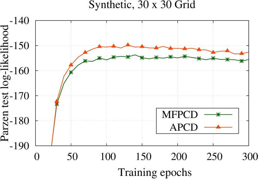
(a) Grid model on synthetic data: Average test log-likelihood of MFPCD and APCD trained model on synthetic dataset in every $10$ epochs.

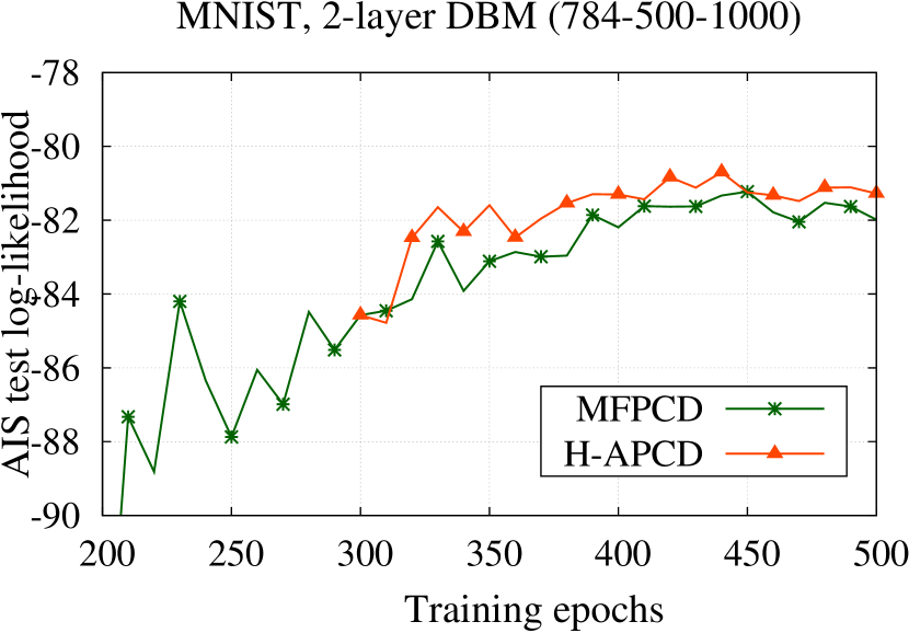
(b) DBM on MNIST: Average test log-likelihood of MFPCD and H-APCD trained model on MNIST dataset in every $10$ epochs.

Figure 1: Generative performances in grid and deep models per training epoch.

4.2 Deep models on real-world datasets

We now report our experimental results of APCD for Deep Boltzmann Machine (DBM). We train two-hidden-layer DBM on the following datasets: MNIST, OCR letters, Frey Face, and Toronto Face (TF). MNIST dataset contains $60,000$ training images and $10,000$ test images of handwritten digits. We use 10,000 images from the training set for validation. OCR letters dataset consists of images of $26$ English characters. The dataset is split into $32,152$ training, $10,000$ validation, and $10,000$ test samples. Frey Face and TF datasets are both real-valued grey-scale images of human faces. While Frey is relatively small, containing $1,965$ images in total, TF contains almost $100,000$ images. For Frey, we use $1,800$ images for training and $10\%$ of the training set as validation. For TF, we follow the splits provided by the dataset.

In order to train a $2$-layer DBM with MFPCD, we follow the same hyperparameter settings as described in [4, 21] for MNIST and OCR. For Frey and TF, the model architecture used in our experiments is $560$-$200$-$400$ and $2304$-$500$-$1000,$ respectively. Pretraining of DBM is performed for 100 epochs over the training set and the global training is done for $500$, $200$, $200$, and $400$ epochs for MNIST, OCR, Frey and TF, with minibatch size of $100$. For M step, the initial learning rate is set to be $0.005$ and decay gradually to $0.0001$ as training progresses. For the DBM experiments, we use Annealed Importance Sampling (AIS) [23] and Parzen window density estimation to measure the average log-likelihood of the test data.

In APCD, we basically follow the same hyperparameters of MFPCD in M step. The E step learning rate starts from a large value close to $1$, and decreases slowly to $0.05$. We also design the following practical hybrid training scheme for DBM, which we call Hybrid APCD (H-APCD). We first train DBM via MFCD in the first halfway in the whole training steps. Then, in the second half, we take the weighted sum of the probabilities computed from APCD and MFPCD, where the ratio of such fusion gradually changes not to favor MFPCD as training progresses. The reason why we take such a hybrid approach of APCD and MFPCD is due to our observation that estimations of E steps in APCD are initially bad in large DBMs due to the mixing issue. We note that for grid graphs in the previous section, such a hybrid training is not necessary since the models are relatively small.

Generative performance. In Table 1, we compare the average test log-likelihood of MFPCD and H-APCD along with other previous works. For MNIST and OCR, we first run AIS $100$ times to estimate the model partition function. Then, we run $100$ AIS runs separately for each test sample to estimate the test log-likelihood. We randomly sample $1,000$ images from the test set to measure the average test log-likelihood. For Frey and TF, we only report Parzen estimates since calculating the log-likelihood using AIS with Gaussian DBM is not straightforward. "True" in Table 1 is computed by running Parzen estimates on 10,000 random samples from the training set. We generate $10,000$ samples from each trained model for Parzen estimates.

Table 1: Generative performances of MFPCD and H-APCD. (a) Test log-likelihood of $1,000$ random samples from the test set measured by running separate $100$ AIS runs per data. (b) Parzen window-based log-likelihood estimates conducted as in [24].

	MNIST	OCR
MFPCD	$-84.31$	$-31.13$
H-APCD	$-83.93$	$-29.59$

(a)

	MNIST	OCR	Frey	TF
DBN[25]	$138\pm 2$	.	.	$1909\pm 66$
Stackted CAE[26]	$121\pm 1.6$	.	.	$2110\pm 50$
Deep GSN[27]	$214\pm 1.1$	.	.	$1890\pm 29$
GAN[24]	$225\pm 2$	.	.	$2057\pm 26$
MFPCD	$239.48\pm 1.7$	$-52.68\pm 0.3$	$659\pm 11$	$1939\pm 28$
H-APCD	$239.24\pm 2.1$	$-52.66\pm 0.4$	$684\pm 11$	$1985\pm 42$
True	$244\pm 1.9$	$-27\pm 0.4$	$931\pm 18$	$2119\pm 23$

(b)

For MNIST and OCR, H-APCD exceeds MFPCD in terms of test log-likelihood of $1,000$ test samples measured by AIS, and performs similarly on Parzen estimates. Figure 1(b) shows the average test log-likelihood of MFPCD and H-APCD trained model in every $10$ epochs on MNIST dataset. The log-likelihood of H-APCD exceeds that of MFPCD after a small amount of training steps and the gap continues to exist until the end of the training. For Frey and TF, H-APCD performs well with a larger margin. The result is comparable to other previous works as well as the true Parzen estimates.

5 Conclusion

In this paper, we propose a new efficient algorithm for parameter learning in graphical models with latent variables. Unlike other known similar methods, it provably converges to a correct optimum. We believe that our techniques based on the multi-time-scale stochastic approximation theory should be of broader interest for designing and analyzing similar algorithms.

Appendix: Proof of Theorem 1

The convergence analysis of the Adiabatic Persistent Contrastive Divergence (APCD) is on the strength of multi-time-scale stochastic approximation theory. As we mentioned in Section 3, our algorithm is interpreted as a stochastic approximation procedure with controlled Markov processes. In this supplementary material, we first provide the convergence analysis of a general stochastic approximation procedure (i.e., with single time-scale) with a controlled Markov process in Section A, where an ordinary differential equation (ODE) is usefully utilized to study the limiting behavior of the system states. Then, in Section B, we non-trivially extend this framework to the APCD algorithm, where the step-size conditions in Theorem 1, controlling the speed of the two dynamics in E and M steps respectively, are the key to the convergence proof.

Appendix A Preliminary: stochastic approximation with controlled Markov process

Consider a discrete-time stochastic process $\{x_{(t)}:t\in\mathbb{Z}_{\geq 0}\}$ with the following form:

$$x_{(t+1)}=x_{(t)}+a_{(t)}\cdot v(x_{(t)},Y_{(t+1)}),\quad\forall t\in\mathbb{Z}_{\geq 0},$$ (13)

where $x_{(t)}\in\mathbb{R}^{L}$ is the system state at the iteration $t$, $a_{(t)}$ corresponds to the step-size, and the system has a Markov process taking values in finite space $\mathcal{Z}$ with control process $x_{(t)}$, i.e., with a controlled transition kernel $K^{x_{(t)}}$. At iteration $t$, the Markov process generates $M$ realizations $\{\hat{z}_{(t+1)}^{m}:m=1,\cdots,M\}$ from the succession of $\ell$ cycles of the transition kernel $K^{x_{(t)}}(\hat{z}_{(t)}^{m},\cdot)$, i.e.,

$$\Pr\left[\hat{z}_{(t+1)}^{m}=z\mid\hat{z}_{(t)}^{m}\right]=(K^{x_{(t)}})^{\ell}\big{(}\hat{z}_{(t)}^{m},z\big{)}.$$

Then, the observation $Y_{(t+1)}$ is a function of the random samples $\{\hat{z}_{(t+1)}^{m}\}$ as:

$$Y_{(t+1)}=\frac{1}{M}\sum_{m=1}^{M}f(\hat{z}_{(t+1)}^{m}).$$

This is often called stochastic approximation with controlled Markov process [9]. We shall assume that if $x_{(t)}=x,\forall t$ for a fixed $x\in\mathbb{R}^{L}$, the Markov process is irreducible and ergodic with unique invariant distribution $\pi^{x}$, and let $\zeta^{x}(\mathrm{d}y)$ denote by the stationary distribution of $\frac{1}{M}\sum_{m=1}^{M}f(\hat{z}^{m})$, where $\{\hat{z}^{m}\}$ are drawn from the Markov process controlled by $x$. In addition, we assume that:

1. For any $x\in\mathbb{R}^{L}$, $x\mapsto K^{x}$ is continuous and $x\mapsto\pi^{x}$ is Lipschitz continuous.

2. The function $f:\mathcal{Z}\mapsto\mathbb{R}^{K}$ is a bounded, and $v(x,Y):\mathbb{R}^{L+K}\mapsto\mathbb{R}^{L}$ is a bounded Lipschitz continuous in $x$ and uniformly over $Y$.

3. Almost surely, $\{x_{(t)}\}$ remains bounded.

4. $\{a_{(t)}\}$ is a decreasing sequence of positive number such that $\sum_{t}a_{(t)}=\infty$ and $\sum_{t}a_{(t)}^{2}<\infty$.

Note that there exist many dynamical MC-based procedures, e.g., Gibbs sampler, Metropolis-Hasting algorithm and variants, which provide property of (C1), and (C3) can be imposed by projecting the process to a bounded subset of $\mathbb{R}^{L}$. The example choices of a step-size (or learning rate) function include $a_{(t)}=\frac{1}{t},\frac{1}{t^{2/3}},\frac{1}{1+t\log t}$.

Now, define $\alpha(t)=\sum_{i=0}^{t-1}a_{(i)}$. We take a continuous-time pairwise linear interpolation of the system state $\{x_{(t)}:t\in\mathbb{Z}_{\geq 0}\}$ under the time-scale $\alpha$ in the following way: define $\{x_{\alpha}(\tau):\tau\in\mathbb{R}_{+}\}$ as: $\forall t\in\mathbb{Z}_{\geq 0}$, for all $\tau\in[\alpha(t),\alpha(t+1))$,

$$x_{\alpha}(\tau)=x_{(t)}+(x_{(t+1)}-x_{(t)})\times\frac{\tau-\alpha(t)}{\alpha(t+1)-\alpha(t)}.$$ (14)

Remark 1.

Intuitively, for a decreasing step-size $a_{(t)}$, the interpolated continuous trajectory $x_{\alpha}(\tau)$ is an accelerated version of the original trajectory $x_{(t)}$. Note that as the decreasing speed of $a_{(t)}$ becomes faster, i.e., $a_{(t)}\rightarrow 0$ at a faster rate, the stochastic process (13) moves on a slower time-scale.

Now, the following theorem provides the convergence analysis of the stochastic approximation procedure with controlled Markov process (13).

Theorem 2 (Theorem 1 of [28], Corollary 8 in Chapter 6.3 of [9]).

Suppose that assumptions (C1)-(C4) hold. Let $T>0$, and denote by $\tilde{x}^{s}(\cdot)$ the solution on $[s,s+T]$ of the following ordinary differential equation (ODE):

$$\dot{x}(\tau)=\int_{y}v(x(\tau),y)\cdot\zeta^{x(\tau)}(\mathrm{d}y),\quad\text{with}\quad\tilde{x}^{s}(s)=x_{\alpha}(s),$$ (15)

Then, we have almost surely,

$$\lim_{s\rightarrow\infty}\sup_{\tau\in[s,s+T]}\|x_{\alpha}(\tau)-\tilde{x}^{s}(\tau)\|=0.$$

Moreover, $x_{(t)}$ converge a.s. to an internally chain transitive invariant set of the ODE (15).

Note that since the Markov process is irreducible and ergodic, and $f$ is continuous and bounded, we have almost surely,

$$\int_{y}v(x,y)\zeta^{x}(\mathrm{d}y)=\sum_{z\in\mathcal{Z}}v(x,f(z))\pi^{x}(z).$$

Therefore, the ODE (15) becomes the following simpler form, which will be used later in the proof of Theorem 1:

$$\dot{x}(\tau) = \sum_{z\in\mathcal{Z}}v(x(\tau),f(z))\pi^{x(\tau)}(z).$$ (16)

Remark 2.

We comment that there exists a slight difference between the model of this section and that of in [28] and [9]: The controlled Markov process is a discrete-time one in our setup, whereas it is a continuous-time one in [9, 28], requiring just a simple modification of the proof.

Theorem 2 states that as time evolves, the dynamics of the underlying Markov process is averaged due to the decreasing step-size, thus “almost reaching the stationary regime”. Thus, it suffices to see how the ODE (16) behaves. In particular, when the ODE (16) has the unique fixed stable equilibrium point $x^{*}$, we have almost surely: $x_{(t)}\to x^{*}$ as $t\to\infty$. If the ODE (16) has a Lyapunov function, then every internally chain transitive invariant lies in the Lyapunov set, and thus the process (13) converges to the largest internally chain transitive invariant set.

Appendix B Proof of Theorem 1

We now prove the convergence of Algorithm 1 by showing that it is a multi-time-scale stochastic approximation procedure with controlled Markov process. We will use some result that works for general multi-time-scale stochastic approximation procedure [9]. To that end, we rewrite E and M step of APCD into following form:

$$\text{{\bf E step:}}\quad\hat{\mu}_{(t+1)} = \hat{\mu}_{(t)}+a_{(t)}\cdot g\bigg{(}\hat{\mu}_{(t)},\theta_{(t)},H_{(t+1)}\bigg{)},$$ (17)

$$\text{{\bf M step:}}\quad\theta_{(t+1)} = \theta_{(t)}+b_{(t)}\cdot u\bigg{(}\hat{\mu}_{(t)},\theta_{(t)},X_{(t+1)}\bigg{)},$$ (18)

where

$$g(\hat{\mu},\theta,H)=H-\hat{\mu},\quad u(\hat{\mu},\theta,X)=\hat{\mu}-X,$$

with

$$H_{(t+1)}=\frac{1}{N}\sum_{n=1}^{N}H_{(t+1)}^{n},\quad H_{(t+1)}^{n}=\frac{1}{M}\sum_{m=1}^{M}\phi(v^{n},\hat{h}_{(t+1)}^{n,m}),\quad X_{(t+1)}=\frac{1}{M}\sum_{m=1}^{M}\phi(\hat{x}_{(t+1)}^{m}).$$

Note that for each visible data $v^{n}$, $\{\hat{h}_{(t+1)}^{n,m}:m=1,\cdots,M\}$ are samples generated from the successive $\ell$ cycles of transition matrix $K_{\theta_{(t)},v^{n}}^{E}$ in E step, and $\{\hat{x}_{(t+1)}^{m}:m=1,\cdots,M\}$ are samples generated from the successive $\ell$ cycles of transition matrix $K_{\theta_{(t)}}^{M}$ in M step. One can easily check that $u(\cdot),g(\cdot)$ are bounded Lipschitz continuous for exponential family with bounded sufficient statistics $\phi$.

We now analyze the coupled stochastic approximation procedures (17) and (18), under the following two “time-scales” with different speed: (i) $\alpha(t)=\sum_{i=0}^{t-1}a_{(i)}$ and (ii) $\beta(t)=\sum_{i=0}^{t-1}b_{(i)}$. We denote by $\{\hat{\mu}_{\alpha}(\tau),\theta_{\alpha}(\tau):\tau\in\mathbb{R}_{+}\}$ and $\{\hat{\mu}_{\beta}(\tau),\theta_{\beta}(\tau):\tau\in\mathbb{R}_{+}\}$ the corresponding continuous-time interpolations of $\{\hat{\mu}_{(t)},\theta_{(t)}:t\in\mathbb{Z}_{\geq 0}\}$ according to (14) for time-scales $\alpha$ and $\beta$, respectively. The condition $\frac{a_{(t)}}{b_{(t)}}\to 0$ or $\frac{a_{(t)}}{b_{(t)}}\to\infty$ in Theorem 1 implies that the decreasing speed of two steps are different: i.e., one step should run in a faster time-scale than the other step. If $\frac{a_{(t)}}{b_{(t)}}\to 0$, E step moves at a slower time-scale than M step, and if $\frac{a_{(t)}}{b_{(t)}}\to\infty$, i.e., equivalently $\frac{b_{(t)}}{a_{(t)}}\to 0$, E step moves at a faster time-scale than M step.

B.1 Case 1: $\frac{a_{(t)}}{b_{(t)}}\to 0$

From the hypothesis $\frac{a_{(t)}}{b_{(t)}}\to 0$, we can first prove the following two properties:

1. For all $T>0$, almost surely,

   $$\lim_{s\to\infty}\sup_{\tau\in[s,s+T]}\|\hat{\mu}_{\beta}(\tau)-\hat{\mu}_{\beta}(s)\|=0.$$ (19)

2. Almost surely,

   $$\lim_{\tau\to\infty}\|\theta_{\alpha}(\tau)-\theta^{*}(\hat{\mu}_{\alpha}(\tau))\|=0.$$

P1 states that $\hat{\mu}_{\beta}(\tau)$ almost behaves like a constant after a sufficient number of iterations. This is due to the fact that $\hat{\mu}_{(t)}$ is updated by the step-size $a_{(t)},$ but $\hat{\mu}_{\beta}(\tau)$ is the trajectory made by the faster time-scale of $b_{(t)}$. More formally, by rewriting (17), we have:

$$\hat{\mu}_{(t+1)} = \hat{\mu}_{(t)}+b_{(t)}\cdot\bigg{[}\frac{a_{(t)}}{b_{(t)}}g\bigg{(}\hat{\mu}_{(t)},\theta_{(t)},H_{(t+1)}\bigg{)}\bigg{]},$$

and thus it is obvious that its limiting ODE is $\dot{\mu}(\tau)=0.$ Then, the property P1 immediately holds. P2 implies that $\theta_{\alpha}(\tau)$ is asymptotically close to a unique fixed point $\theta^{*}(\hat{\mu}_{\alpha}(\tau))$, a MLE parameter in (4) for a given empirical mean parameter $\hat{\mu}_{\alpha}(\tau)$. Note that for a regular and minimal exponential family, the map $\theta^{*}(\cdot)$ is a bijection mapping, see Section 2.1. In the rest of the proof, we first show P2 in Step 1, and then in Step 2, we complete the proof of Case 1 using P1 and P2.

Step 1: Understanding the asymptotic behavior of the system at the faster time-scale $\beta$.

We now introduce $\{\theta_{\beta}^{s}(\tau):\tau\in\mathbb{R}_{+}\}$, which interpolates $\{\theta_{(t)}^{s}:t\in\mathbb{Z}_{\geq 0}\}$ (similarly to (14)), where $\{\theta_{(t)}^{s}:t\in\mathbb{Z}_{\geq 0}\}$ is constructed such that with $s\in\mathbb{R}$, $\theta_{(t)}^{s}=\theta_{(t)}$ for $s\geq\beta(t)$, and

$$\theta^{s}_{(t+1)}=\theta^{s}_{(t)}+b_{(t)}\cdot u\bigg{(}\hat{\mu}_{\beta}(s),\theta^{s}_{(t)},X_{(t+1)}\bigg{)},$$ (20)

for $s<\beta(t)$. Note that (20) is different to (18) in that $\hat{\mu}_{(t)}$ is fixed to $\hat{\mu}_{\beta}(s)$. Then, from the Lipschitz continuity of $u(\cdot)$, we get that for all $T>0$:

$$\lim_{s\to\infty}\sup_{\tau\in[s,s+T]}\|\theta_{\beta}^{s}(\tau)-\theta_{\beta}(\tau)\|=0.$$ (21)

Now, we will compare $\theta_{\beta}^{s}(\tau)$ to the solution trajectory of the following ODE, as in (16) of Section A:

$$\dot{\theta}(\tau)=u^{\dagger}(\theta(\tau))\mathrel{:=}\sum_{x\in\mathcal{X}}u\bigg{(}\hat{\mu}_{\beta}(s),\theta(\tau),\phi(x)\bigg{)}p_{\theta(\tau)}(x).$$ (22)

To explain how our setup matches with that in Section A, let $\tilde{\theta}^{s}(\tau)$ be the solution on $[s,s+T]$ (for $T>0$) of the ODE (22) with $\tilde{\theta}^{s}(s)=\theta_{\beta}^{s}(s)$. It is clear that $\{\theta_{(t)}^{s}:t\in\mathbb{Z}_{\geq 0}\}$ is a discrete-time stochastic process with controlled Markov process considered in (13) for $s\leq\beta(t)$. We can verify that the assumptions (C1)-(C4) are satisfied. First, the MC sampler in M step $K_{\theta}^{M}$ induces an ergodic Markov chain taking values in a finite set $\mathcal{X}$, which satisfies the detailed balance property with respect to $p_{\theta}(x)$ in (1) for a fixed $\theta\in\Theta$, e.g., Gibbs sampler. (C1) is verified with our choice of $K_{\theta}^{M}$. (C2) is verified since sufficient statistics $\phi$ is bounded. (C3) is the assumption of Theorem 1, where some techniques for establishing this stability condition has been studied, see Chapter 3 of [9]. Finally, (C4) is verified with our choice of $b_{(t)}$. Then, we have that for all $T>0$,

$$\lim_{s\rightarrow\infty}\sup_{\tau\in[s,s+T]}\|\theta_{\beta}(\tau)-\tilde{\theta}^{s}(\tau)\|=0,\quad\text{ a.s.}.$$

This is a direct consequence of Theorem 2 and (21).

Now, for any regular and minimal exponential family, the ODE system (22) has a unique fixed point $\theta^{*}=\theta^{*}(\hat{\mu}_{\beta}(s))$, i.e., a MLE parameter in (4) for a given empirical mean parameter $\hat{\mu}_{\beta}(s)$, due to the fact that

$$u^{\dagger}(\theta(\tau))=\hat{\mu}_{\beta}(s)-\mathbb{E}_{\theta(\tau)}[\phi(X)]=\nabla l(\theta(\tau);\hat{\mu}_{\beta}(s)).$$

Then, we apply the following Lemma in Chapter 6.1 of [9]:

Lemma B.1 (Lemma 1 in Chapter 6.1 of [9]).

$$(\hat{\mu}_{(t)},\theta_{(t)})\rightarrow\{(\hat{\mu},\theta^{*}(\hat{\mu})):\hat{\mu}\in\mathcal{M}^{\circ}\},\quad\text{ a.s.}.$$

In other words, we have almost surely,

$$\|\theta_{(t)}-\theta^{*}(\hat{\mu}_{(t)})\|\rightarrow 0,$$ (23)

which in turn implies that under the slower time-scale $\alpha$, we also have almost surely,

$$\lim_{\tau\to\infty}\|\theta_{\alpha}(\tau)-\theta^{*}(\hat{\mu}_{\alpha}(\tau))\|=0.$$ (24)

This completes the proof of P2.

Step 2. Understanding the asymptotic behavior of the system at the slower time-scale $\alpha$.

We start by introducing $\{\hat{\mu}_{\alpha}^{s}(\tau);\tau\in\mathbb{R}_{+}\}$ (similar to $\theta_{\beta}^{s}(\tau)$ in Step 1), which interpolates $\{\hat{\mu}_{(t)}^{s}:t\in\mathbb{Z}_{\geq 0}\}$, where it is constructed such that with $s\in\mathbb{R}$, $\hat{\mu}_{(t)}^{s}=\hat{\mu}_{(t)}$ for $s\geq\alpha(t)$, and

$$\hat{\mu}^{s}_{(t+1)}=\hat{\mu}^{s}_{(t)}+a_{(t)}\cdot g\bigg{(}\hat{\mu}^{s}_{(t)},\theta^{*}(\hat{\mu}^{s}_{(t)}),H_{(t+1)}\bigg{)},$$

for $s<\alpha(t)$. Note that (B.1) is different to (17) in that $\theta_{(t)}$ is fixed to $\theta^{*}(\hat{\mu}_{(t)}^{s})$. Then, from (24) and the fact that $g(\cdot)$ is Lipschitz continuous, it follows that for all $T>0$,

$$\lim_{s\to\infty}\sup_{\tau\in[s,s+T]}\|\hat{\mu}_{\alpha}^{s}(\tau)-\hat{\mu}_{\alpha}(\tau)\|=0.$$ (25)

Now, we compare $\hat{\mu}_{\alpha}^{s}(\tau)$ to the solution trajectory of the following ODE, as in Section A:

$$\dot{\mu}(\tau)=g^{\dagger}(\mu(\tau))\mathrel{:=}\sum_{h\in\mathcal{X}^{h}}g\bigg{(}\mu(\tau),\theta^{*}(\mu(\tau)),\phi(\mathbf{v},h)\bigg{)}p_{\theta^{*}(\mu(\tau))}(h|\mathbf{v}).$$ (26)

It is clear that the process $\{\hat{\mu}_{(t)}^{s}:t\in\mathbb{Z}_{\geq 0}\}$ is also a discrete-time stochastic process with controlled Markov process considered in (13) for $s\leq\alpha(t)$. The assumptions (C1)-(C4) are verified as follows: The MC sampler in E step $K_{\theta,\mathbf{v}}^{E}$ induces an ergodic Markov chain taking values in a finite set $\mathcal{X}^{h}$, which satisfies the detailed balance property with respect to $p_{\theta}(h|\mathbf{v})$ for a fixed $\theta\in\Theta$, e.g., Gibbs sampler. With our choice of $K_{\theta,\mathbf{v}}^{E}$, since $\phi$ is bounded and $\theta^{*}(\cdot)$ is continuous, we have $\hat{\mu}\mapsto p_{\theta^{*}(\hat{\mu})}(h|\mathbf{v})$ and becomes Lipschitz continuous, i.e., (C1) is verified. (C2),(C3) are verified since $\phi$ is bounded. Finally, (C4) is verified with our choice of $a_{(t)}$. Let denote by $\tilde{\mu}^{s}(\tau)$ be the solution on $[s,s+T]$ (for any $T>0$) of the ODE (26) with $\tilde{\mu}^{s}(s)=\hat{\mu}_{\alpha}^{s}(s)$. Then, we now have that for all $T>0$,

$$\lim_{s\rightarrow\infty}\sup_{\tau\in[s,s+T]}\|\hat{\mu}_{\alpha}(\tau)-\tilde{\mu}^{s}(\tau)\|=0,\quad\text{ a.s.},$$

which is a direct consequence of Theorem 2 and (25).

Next, we claim that there exists a Lyapunov function of the ODE (26).

Lemma B.2.

Assume that exponential family $(\theta,\phi)$ has regularity, minimality and bounded sufficient statistics. Then, $V(\hat{\mu})=-l(\theta^{*}(\hat{\mu});\mathbf{v})$ is a Lyapunov function of the ODE (26): i.e., $V(\hat{\mu})$ is a function such that

1. For all $\hat{\mu}\in\mathcal{M}$, $F(\hat{\mu})\mathrel{:=}\langle\partial_{\hat{\mu}}V(\hat{\mu}),g^{\dagger}(\hat{\mu})\rangle\leq 0$,

2. $V(\{\hat{\mu}:F(\hat{\mu})=0\})$ has an empty interior.

Moreover,

$$\{\hat{\mu}:F(\hat{\mu})=0\}=\{\hat{\mu}:\partial_{\hat{\mu}}V(\hat{\mu})=0\}\quad\mbox{and}\quad\theta^{*}(\{\hat{\mu}:F(\hat{\mu})=0\})=\{\theta\in\Theta:\partial_{\theta}l(\theta;\mathbf{v})=0\}.$$

Remark 3.

Lemma B.2 is an application of Lemma 2 presented in [10], which gives a result about Lyapunov function of the ODE system of the form (26). We omit the formal proof of Lemma B.2 since the assumptions of Lemma 2 in [10] are shortly verified for a regular and minimal exponential family with bounded sufficient statistics.

We now use the following result in [9] at our framework to discuss the convergence guarantee of $\{\hat{\mu}_{(t)}:t\in\mathbb{Z}_{\geq 0}\}$ and the convergence point characterization.

Lemma B.3 (Corollary 3 in Chapter 2.2 of [9]).

Under the assumption that $\{\hat{\mu}_{(t)}\}$ remains bounded, $\{\hat{\mu}_{(t)}\}$ almost surely converges to an internally chain transitive invariant set contained in $\{\hat{\mu}\in\mathcal{M}^{\circ}:F(\hat{\mu})=0\}$.

By Lemma B.2 and Lemma B.3, it follows that

$$\hat{\mu}_{(t)}\rightarrow\{\hat{\mu}:\partial_{\hat{\mu}}V(\hat{\mu})=0\},\quad\text{ a.s.}.$$ (27)

This completes the proof of Step 2.

Combining Step 1 and Step 2, i.e., from (23) and (27), we complete the proof for Case 1 of Theorem 1 that under APCD, $\theta_{(t)}$ almost surely converges to a stationary point of MMLE: i.e.,

$$\theta_{(t)}\rightarrow\{\theta:\partial_{\theta}l(\theta;\mathbf{v})=0\},\text{ a.s.}.$$

B.2 Case 2: $\frac{a_{(t)}}{b_{(t)}}\to\infty$

In Case 2, we have following two properties:

1. For all $T>0$, almost surely,

   $$\lim_{s\to\infty}\sup_{\tau\in[s,s+T]}\|\theta_{\alpha}(\tau)-\theta_{\alpha}(s)\|=0.$$ (28)

2. Almost surely,

   $$\lim_{\tau\to\infty}\|\hat{\mu}_{\beta}(\tau)-\hat{\mu}^{*}(\theta_{\beta}(\tau);\mathbf{v})\|=0.$$

P1 states that $\theta_{\alpha}(\tau)$ almost behaves like a constant after a sufficient number of iterations. This is due to the fact that $\theta_{(t)}$ is updated by the step-size $b_{(t)}$, but $\theta_{\alpha}(\tau)$ is the trajectory made by the slower time-scale of $a_{(t)}$. More formally, rewriting (17), we have:

$$\theta_{(t+1)} = \theta_{(t)}+a_{(t)}\cdot\bigg{[}\frac{b_{(t)}}{a_{(t)}}u\bigg{(}\hat{\mu}_{(t)},\theta_{(t)},X_{(t+1)}\bigg{)}\bigg{]},$$

and thus it is obvious that its limiting ODE is $\dot{\theta}(\tau)=0$. Then, the property P1 immediately holds. P2 implies that $\hat{\mu}_{\beta}(\tau)$ is asymptotically close to a unique fixed point $\hat{\mu}^{*}(\theta_{\beta}(\tau);\mathbf{v})$, the expectation of empirical mean parameter over the distribution $p_{\theta_{\beta}(\tau)}(h|\mathbf{v})$ for a given $\theta_{\beta}(\tau)$ and $\mathbf{v}$. It is clear that the map $\hat{\mu}^{*}(\cdot;\mathbf{v})$ is a bijection for a regular and minimal exponential family. In the rest of the proof, as in Case 1, we first show P2 in the first step, and then in the second step, we complete the proof using P1 and P2.

Step 1: Understanding the asymptotic behavior of the system at the faster time-scale $\alpha$.

We introduce $\{\hat{\mu}_{\alpha}^{s}(\tau):\tau\in\mathbb{R}_{+}\}$, which interpolates $\{\hat{\mu}_{(t)}^{s}:t\in\mathbb{Z}_{\geq 0}\}$, where $\{\hat{\mu}_{(t)}^{s}:t\in\mathbb{Z}_{\geq 0}\}$ is constructed such that with $s\in\mathbb{R}$, $\hat{\mu}_{(t)}^{s}=\hat{\mu}_{(t)}$ for $s\geq\alpha(t)$, and

$$\hat{\mu}_{(t+1)}^{s}=\hat{\mu}_{(t)}^{s}+a_{(t)}\cdot g\bigg{(}\hat{\mu}_{(t)}^{s},\theta_{\alpha}(s),H_{(t+1)}\bigg{)},$$ (29)

for $s<\alpha(t)$. Note that (29) is slightly different to (17) in that $\theta_{(t)}$ is fixed to $\theta_{\alpha}(s)$. Then, from the Lipschitz continuity of $g(\cdot)$, we get that for all $T>0$:

$$\lim_{s\to\infty}\sup_{\tau\in[s,s+T]}\|\hat{\mu}_{\alpha}^{s}(\tau)-\hat{\mu}_{\alpha}(\tau)\|=0.$$ (30)

Now, we will compare $\hat{\mu}_{\alpha}^{s}(\tau)$ to the solution trajectory of the following ODE, as in Section A:

$$\dot{\mu}(\tau)=g^{\ddagger}(\mu(\tau))\mathrel{:=}\sum_{h\in\mathcal{X}^{h}}g\bigg{(}\mu(\tau),\theta_{\alpha}(s),\phi(\mathbf{v},h)\bigg{)}p_{\theta_{\alpha}(s)}(h|\mathbf{v}).$$ (31)

To see how the setup matches with that in Section A, let $\tilde{\mu}^{s}(\tau)$ be the solution on $[s,s+T]$ (for $T>0$) of the ODE (31) with $\tilde{\mu}^{s}(s)=\hat{\mu}_{\alpha}^{s}(s)$. Then, $\{\hat{\mu}_{(t)}^{s}:t\in\mathbb{Z}_{\geq 0}\}$ is a discrete-time stochastic process with controlled Markov process considered in (13) for $s\leq\alpha(t)$. We can verify that the assumptions (C1)-(C4) are satisfied as we verified in the proof for Case 1. Then, we have that for all $T>0$,

$$\lim_{s\to\infty}\sup_{\tau\in[s,s+T]}\|\hat{\mu}_{\alpha}(\tau)-\tilde{\mu}^{s}(\tau)\|=0,\quad\text{ a.s.},$$

which is a direct consequence of Theorem 2 and (30).

Here, it is clear that the ODE system (31) has a unique fixed point $\hat{\mu}^{*}=\hat{\mu}^{*}(\theta_{\alpha}(s);\mathbf{v})$, i.e., the expectation of empirical mean parameter over $p_{\theta_{\alpha}(s)}(\cdot|\mathbf{v})$, from the fact that

$$g^{\ddagger}(\mu(\tau))=\mathbb{E}_{\theta_{\alpha}(s),\mathbf{v}}[\phi(\mathbf{v},H)]-\mu(\tau).$$

Then, by applying Lemma B.1 to this framework we have almost surely,

$$\|\hat{\mu}_{(t)}-\hat{\mu}^{*}(\theta_{(t)};\mathbf{v})\|\to 0,$$ (32)

which in turn implies that under the slower time-scale $\beta$, we also have almost surely,

$$\lim_{\tau\to\infty}\|\hat{\mu}_{\beta}(\tau)-\hat{\mu}^{*}(\theta_{\beta}(\tau);\mathbf{v})\|=0.$$ (33)

This completes the proof of P2.

Step 2. Understanding the asymptotic behavior of the system at the slower time-scale $\beta$.

We start by introducing $\{\theta_{\beta}^{s}(\tau):\tau\in\mathbb{R}_{+}\}$, which interpolates $\{\theta_{(t)}^{s}:t\in\mathbb{Z}_{\geq 0}\}$, where it is constructed such that with $s\in\mathbb{R}$, $\theta_{(t)}^{s}=\theta_{(t)}$ for $s\geq\beta(t)$, and

$$\theta_{(t+1)}^{s}=\theta_{(t)}^{s}+b_{(t)}\cdot u\bigg{(}\hat{\mu}^{*}(\theta_{(t)}^{s};\mathbf{v}),\theta_{(t)}^{s},X_{(t+1)}\bigg{)}$$ (34)

for $s<\beta(t)$. Note that (34) is slightly different to (18) in that $\hat{\mu}_{(t)}$ is fixed to $\hat{\mu}^{*}(\theta_{(t)}^{s};\mathbf{v})$. Then, from (33) and the Lipschitz continuity of $u(\cdot)$, it follows that for all $T>0$,

$$\lim_{s\to\infty}\sup_{\tau\in[s,s+T]}\|\theta_{\beta}^{s}(\tau)-\theta_{\beta}(\tau)\|=0.$$ (35)

Next, we compare $\theta_{\beta}^{s}(\tau)$ to the solution trajectory of the following ODE:

$$\dot{\theta}(\tau)=u^{\ddagger}(\theta(\tau))\mathrel{:=}\sum_{x\in\mathcal{X}}u\bigg{(}\hat{\mu}^{*}(\theta(\tau);\mathbf{v}),\theta(\tau),\phi(x)\bigg{)}p_{\theta(\tau)}(x).$$ (36)

It is clear that the process $\{\theta_{(t)}^{s}\}$ is also a discrete-time stochastic process with controlled Markov process in Section A for $s\leq\beta(t)$. The assumptions (C1)-(C4) are verified similarly in Case 1. Let denote by $\tilde{\theta}^{s}(\tau)$ be the solution on $[s,s+T]$ (for any $T>0$) of the ODE (36) with $\tilde{\theta}^{s}(s)=\theta_{\beta}^{s}(s)$. Then, we have that for all $T>0$,

$$\lim_{s\to\infty}\sup_{\tau\in[s,s+T]}\|\theta_{\beta}(\tau)-\tilde{\theta}^{s}(\tau)\|=0,\quad\text{ a.s.},$$

which is a direct result from Theorem 2 and (35).

Remark 4.

We can shortly claim that $V(\theta)=-l(\theta;\hat{\mu}^{*}(\theta;\mathbf{v}))$ is a Lyapunov function of the ODE (36), by checking the definition of Lyapunov function in [9]. Moreover, $l(\theta;\hat{\mu}^{*}(\theta;\mathbf{v}))=l(\theta;\mathbf{v})$, which is the exact bound of the marginal log-likelihood in (6).

Then, we plug the process $\{\theta_{(t)}:t\in\mathbb{Z}_{\geq 0}\}$ and ODE (36) into Lemma B.3, i.e., convergence analysis of stochastic approximation procedure with Lyapunov function, and we have that:

$$\theta_{(t)}\to\{\theta:\partial_{\theta}l(\theta;\mathbf{v})=0\},\quad\text{ a.s.}.$$ (37)

This completes the proof of Step 2. Combining Step 1 and Step 2, i.e., from (32) (37), completes the proof for Case 2.

Finally, for both Case 1 and Case 2, we conclude that under APCD, $\theta_{(t)}$ almost surely converges to a stationary point of MMLE, i.e.,

$$\theta_{(t)}\rightarrow\{\theta:\partial_{\theta}l(\theta;\mathbf{v})=0\},\quad\text{ a.s.},$$

which completes the proof of Theorem 1. ∎

References

- [1] M. Welling and G. E. Hinton. A new learning algorithm for mean field boltzmann machines. In Artificial Neural Networks—ICANN 2002, pages 351–357. Springer, 2002.
- [2] T. Tieleman. Training restricted boltzmann machines using approximations to the likelihood gradient. In Proceedings of the International Conference on Machine Learning, pages 1064–1071, 2008.
- [3] P. Smolensky. Information processing in dynamical systems: Foundations of harmony theory. In D. E. Rumelhart, J. L. McClelland, et al., editors, Parallel Distributed Processing, pages 194–281. MIT Press, 1987.
- [4] R. Salakhutdinov and G. E. Hinton. Deep boltzmann machines. In Proceedings of the International Conference on Artificial Intelligence and Statistics, pages 448–455, 2009.
- [5] H. Larochelle and Y. Bengio. Classification using discriminative restricted boltzmann machines. In Proceedings of the International Conference on Machine Learning, pages 536–543, 2008.
- [6] G. Dahl, A. R. Mohamed, and G. E. Hinton. Phone recognition with the mean-covariance restricted boltzmann machine. In Proceedings of the Advances in Neural Information Processing Systems, pages 469–477, 2010.
- [7] R. Salakhutdinov, A. Mnih, and G. E. Hinton. Restricted boltzmann machines for collaborative filtering. In Proceedings of the International Conference on Machine Learning, pages 791–798, 2007.
- [8] M. Born and V. A. Fock. Beweis des adiabatensatzes. Zeitschrift fur Physik a Hadrons and Nuclei, 51(3-4):165–180, 1928.
- [9] V. S. Borkar, editor. Stochastic Approximation: A Dynamical Systems Viewpoint. Cambridge University Press, 2008.
- [10] B. Delyon, M. Lavielle, and E. Moulines. Convergence of a stochastic approximation version of the EM algorithm. Annals of Statistics, 27(1):94–128, 1999.
- [11] E. Kuhn and M. Lavielle. Coupling a stochastic approximation version of EM with an mcmc procedure. ESAIM: Probability and Statistics, 8:115–131, 2004.
- [12] L. Younes. On the convergence of markovian stochastic algorithms with rapidly decreasing ergodicity rates. Stochastics: An International Journal of Probability and Stochastic Processes, 65(3-4):177–228, 1999.
- [13] A. Yuille. The convergence of contrastive divergences. In Proceedings of the Advances in Neural Information Processing Systems, 2004.
- [14] I. Sutskever and T. Tieleman. On the convergence properties of contrastive divergence. In Proceedings of the International Conference on Artificial Intelligence and Statistics, pages 789–795, 2010.
- [15] E. Marinari and G. Parisi. Simulated tempering: a new Monte Carlo scheme. EPL (Europhysics Letters), 19(6):451, 1992.
- [16] G. Desjardins, A. Courville, Y. Bengio, P. Vincent, and O. Delalleau. Tempered Markov chain Monte Carlo for training of restricted Boltzmann machines. In Proceedings of the International Conference on Artificial Intelligence and Statistics, pages 145–152, 2010.
- [17] R. Salakhutdinov. Learning in Markov random fields using tempered transitions. In Proceedings of the Advances in Neural Information Processing Systems, pages 1598–1606, 2009.
- [18] K. Cho, T. Raiko, and A. Ilin. Parallel tempering is efficient for learning restricted Boltzmann machines. In Proceedings of the International Joint Conference on Neural Networks, pages 1–8, 2010.
- [19] R. Salakhutdinov. Learning deep Boltzmann machines using adaptive MCMC. In Proceedings of the International Conference on Machine Learning, pages 943–950, 2010.
- [20] O. Breuleux, Y. Bengio, and P. Vincent. Quickly generating representative samples from an rbm-derived process. Neural Computation, 23(8):2058–2073, 2011.
- [21] R. Salakhutdinov and H. Larochelle. Efficient learning of deep botlzmann machines. In Proceedings of the International Conference on Artificial Intelligence and Statistics, pages 693–700, 2010.
- [22] V. Nair and G. E. Hinton. Implicit mixtures of restricted boltzmann machines. In Proceedings of the Advances in Neural Information Processing Systems, pages 1145–1152, 2009.
- [23] R. M. Neal. Annealed importance sampling. Statistics and Computing, 11(2):125–139, 2001.
- [24] I. Goodfellow, J. Pouget-Abadie, M. Mirza, B. Xu, D. Warde-Farley, S. Ozair, A. Courville, and Y. Bengio. Generative adversarial nets. In Proceedings of the Advances in Neural Information Processing Systems, pages 2672–2680, 2014.
- [25] G. E. Hinton, S. Osindero, and Y. Teh. A fast learning algorithm for deep belief nets. Neural computation, 18(7):1527–1554, 2006.
- [26] Y. Bengio, G. Mesnil, Y. Dauphin, and S. Rifai. Better mixing via deep representations. In Proceedings of the International Conference on Machine Learning, pages 552–560, 2013.
- [27] Y. Bengio, E. Laufer, G. Alain, and J. Yosinski. Deep generative stochastic networks trainable by backprop. In Proceedings of the International Conference on Machine Learning, pages 226–234, 2014.
- [28] A. Proutiere, Y. Yi, T. Lan, and M. Chiang. Resource allocation over network dynamics without timescale separation. In Proceedings of the 29th Conference on Information Communications (INFOCOM 2010), pages 406–410. IEEE Press, 2010.