Multiple target tracking based on sets of trajectories

Abstract

We propose a solution of the multiple target tracking (MTT) problem based on sets of trajectories and the random finite set framework. A full Bayesian approach to MTT should characterise the distribution of the trajectories given the measurements, as it contains all information about the trajectories. We attain this by considering multi-object density functions in which objects are trajectories. For the standard tracking models, we also describe a conjugate family of multitrajectory density functions.

I Introduction

Multiple target tracking (MTT) has an extensive range of applications, for example, in surveillance [1], robotics [2] or computer vision [3]. In MTT, sensors obtain noisy measurements from targets that appear, move and disappear from a scene of interest, forming trajectories or tracks. In MTT, we are interested in answering target and trajectory-related questions that may arise in the application under consideration. For example, what are the best target estimates at the current time (according to a certain criterion)? What are the best trajectory estimates? As illustrated in Figure 1, after two planes fly around for some time, what is the probability that the same plane was in city A at a certain time and is in city B now?

From a Bayesian perspective, after observing noisy measurements from a random variable, all available knowledge about this random variable is included in its conditional distribution given the measurements [4]. Therefore, this distribution enables us to answer all possible questions about the considered random variable. In this paper, we are interested in how to represent this variable/state in MTT and how to characterise its distribution so that we have a full Bayesian solution of the MTT problem and can answer all types of target and trajectory related questions. We focus on the MTT problem with targets without a unique identification. That is, there is not a unique way in which a particular target moves or affects measurements, which is the common case in radar applications [5, 6, 7, 8]. We proceed to review state representations used in the literature, along with their pros and cons, before stating our contributions and their practical implications.

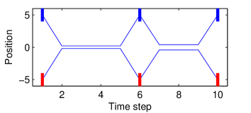
Figure 1: Illustration of a trajectory-related question in one-dimensional case. Two targets are initially separated, get in close proximity and separate twice, as represented by thin blue lines. A possible trajectory-related question is, what is the probability that the same target (plane) was in interval (city) $A=\left[4,6\right]$, shown as a thick blue line, at time 6 and in interval $B=\left[-4,-6\right]$, shown as a thick red line, at time 10?

Original derivations of classic MTT algorithms, such as multiple hypothesis tracking (MHT) [5] and joint probabilistic data association (JPDA) [9] do not explicitly use a representation of the multitarget state. Nevertheless, later papers on MHT and JPDA represent the multitarget state at a certain time step as a vector or a sequence [10, 11, 6]. A set representation [8, 12] in multi-object systems has some advantages over vector/sequence representation: we avoid the arbitrary ordering of the objects inherent in the multi-object state vector/sequence and we can define mathematical metrics for algorithm evaluation and estimator design [13, 14].

An appealing and rigorous way of dealing with such multiple object systems from a Bayesian point of view is to use the random finite set (RFS) framework and finite-set statistics (FISST) developed by Mahler [8, 12]. In the proposed RFS algorithms for MTT, the state at a certain time step is the (random) set of targets at this time step and, as in classic approaches to MTT, the main focus has been on the filtering problem. That is, we recursively calculate/approximate the multitarget density of the current set of targets given current and past measurements [12]. This density is referred to as the multitarget filtering density and contains all information of interest about the targets at the current time. Based on the multitarget filtering densities, we can answer target-related questions at the current time step, such as target state estimation. However, we cannot answer trajectory-related questions, such as the one illustrated in Figure 1, and it is not obvious how to build trajectories in a sound manner.

The most popular approach to try to build trajectories from first principles consists of adding a unique label to each single target state so that each target is identified over its life time [15, 16, 17, 18, 19, 20, 21, 22][8, Sec. 14.5.6], though other approaches exist [23]. Labels can appear in two forms. If a label is explicit, such as the registration number of an aircraft or the name of a person, labels may have a physical meaning and are referred to as target IDs. However, in many cases, these target IDs are not observable [5, 6, 7, 8] and there is total uncertainty about them. For example, it is not possible to infer the serial number of a missile using radar measurements and it is not usually of interest.

When IDs cannot be inferred and therefore do not form part of the model, as in this paper, one approach to build trajectories is to add implicit labels, which we simply refer to as labels, rather than the explicit labels. In this case, labels are unobservable, static and uniquely assigned to targets when they are born following a certain convention. In a deterministic setting, labels allow us to identify trajectories from a sequence of sets of labelled targets. However, instead of computing the joint posterior distribution of the sequence of sets of labelled targets, the usual approach in MTT is to build trajectories based on the labeled multi-target filtering (or smoothing) densities, i.e., the marginal distributions of these sets.

Considering multi-target densities rather than the joint posterior distribution, as required in a full Bayesian solution to MTT, has the advantage of requiring lower computational resources. Yet, because the joint posterior distribution of the trajectories is not contained in multi-target densities, some problematic cases can arise. For instance, when new born targets are an independent and identically distributed (IID) cluster RFS or Poisson RFS [12, 24], labelled multitarget densities show total uncertainty in the associations between labels and targets born at the same time, as will be explained in Section II-B. This label association uncertainty implies that there can be a never ending track-switching in the estimates for targets born at the same time unless some ad-hoc mechanism is used.

The above-mentioned problems of MTT based on labelled multitarget densities can be solved by considering the joint density on the sequence of sets of labelled targets at all time steps, as pointed out in [18, Sec. II.B] and used in [25]. This density is a valid representation of the posterior distribution of the trajectories. Based on it, we can answer all possible trajectory-related questions and optimally estimate trajectories. However, as we will see, there is no need to artificially identify targets through labelling, which increases the dimension of the state, to estimate trajectories or answer trajectory-related questions. Moreover, the arbitrariness of the labels prevents the development of metrics with physical interpretation on the space of sequences of labelled sets, as will be explained in Section II-B.

In this paper, we propose the set of trajectories as the variable of interest in MTT. In the standard dynamic model, targets are born, move and die [8] so a target trajectory is characterised by a start time, a length and a sequence of target states. A set of trajectories provides a minimal, unambiguous representation of the MTT system at all time steps without arbitrary variables. This representation enables us to define metrics with physical interpretation, such as the ones in [26, 27], which are important for evaluating algorithms and estimator design. Applying Mahler’s RFS framework [12] to MTT with sets of trajectories, we explain how to characterise a distribution over sets of trajectories using a multitrajectory density, which corresponds to a multiobject density in which the objects are trajectories. All information of interest about the trajectories up to the current time is therefore contained in the multitrajectory density given the available measurements. Importantly, this multitrajectory density has significantly fewer terms than a corresponding joint density over the sequence of labelled sets, as will be analysed in Section II-B.

One way of computing the required multitrajectory density is by using the filtering equations with the set of trajectories as state variable. The adoption of the set of trajectories as state variable constitutes a natural and elegant analog of the RFS approach for multitarget filtering, in which we aim to estimate the current set of targets, to multitarget tracking. This representation therefore enables us to extend algorithms for multitarget filtering, such as the probability hypothesis density (PHD) filter [28], to multitarget tracking: the trajectory PHD filter [29]. Obviously, dealing with multitrajectory densities is more challenging than dealing with multitarget densities. Nevertheless, we think it is important to properly characterise the full MTT problem in a Bayesian context. This is an important preliminary step to develop approximations/algorithms that are suitable for answering the trajectory-related questions that arise in different applications. Therefore, the main purpose of this paper is to establish the theoretical foundations to perform MTT using sets of trajectories, not the development of efficient, practical algorithms.

In this paper, we also present the filtering equations and a conjugate family of densities, in the spirit of [17], for computing the multitrajectory filtering density. Finally, we also establish the relation between the multitrajectory filtering density and the multitarget filtering density. Preliminary results on sets of trajectories were provided in [30].

The rest of the paper is organised as follows. In Section II, we define a set of trajectories and motivate its use as the state variable. In Section III, we provide the recursive equations to calculate the multitrajectory filtering density. We analyse the relations among the proposed approach, labelled approaches, the usual RFS tracking framework based on sets of targets and classical MHT in Section IV. Two illustrative examples are provided in Section V and concluding remarks are given in Section VI.

II Sets of trajectories

In this section, we introduce the variables, motivate why we propose the set of trajectories as a state variable and indicate how to use FISST for sets of trajectories.

II-A State variables and notation

A single target state $x\in D$, where $D=\mathbb{R}^{n_{x}}$, contains the information of interest about the target, e.g., its position and velocity. A set $\mathbf{x}$ of single target states belongs to $\mathcal{F}\left(D\right)$ where $\mathcal{F}\left(D\right)$ denotes the set of all finite subsets of $D$. We are interested in representing the information on all target trajectories, where a trajectory consists of a sequence of target states that can start at any time step and end at any time after it starts. Mathematically, a trajectory is represented as a variable $X=\left(t,x^{1:i}\right)$ where $t$ is the initial time step of the trajectory, $i$ is its length and $x^{1:i}=\left(x^{1},...,x^{i}\right)$ denotes a sequence of length $i$ that contains the target states at consecutive time steps of the trajectory.

We consider trajectories up to some finite time step $k^{\prime}$. As a trajectory $\left(t,x^{1:i}\right)$ exists from time step $t$ to $t+i-1$, variable $\left(t,i\right)$ belongs to the set $I_{(k^{\prime})}=\left\{\left(t,i\right):0\leq t\leq k^{\prime}\,\mathrm{and}\,1\leq i\leq k^{\prime}-t+1\right\}$. A single trajectory $X$ up to time step $k^{\prime}$ therefore belongs to the space $T_{\left(k^{\prime}\right)}=\uplus_{\left(t,i\right)\in I_{(k^{\prime})}}\left\{t\right\}\times D^{i}$, where $D^{i}$ represents $i$ Cartesian products of $D$ and $\uplus$ stands for disjoint union, which is used in this paper to highlight that it is the union of disjoint sets. Similarly to the set ${\bf x}$ of targets, we denote a set of trajectories up to time step $k^{\prime}$ as $\mathbf{X}\in\mathcal{F}\left(T_{\left(k^{\prime}\right)}\right)$.

Given a single target trajectory $X=\left(t,x^{1:i}\right)$, the set $\tau^{k}\left(X\right)$ of the target state at time $k$ is

$$\tau^{k}\left(X\right)=\begin{cases}\left\{x^{k+1-t}\right\}&t\leq k\leq t+i-1\\ \emptyset&\mathrm{elsewhere}.\end{cases}$$

As the trajectory exists from time step $t$ to $t+i-1$, the set is empty if $k$ is outside this interval. We employ the following terminology:

• A trajectory $X$ is present at time step $k$ if and only if $\left|\tau^{k}\left(X\right)\right|=1$.

• A surviving trajectory at time $k$ is a trajectory that is present at times $k$ and $k-1$.

Given a set $\mathbf{X}$ of trajectories, the set $\tau^{k}\left(\mathbf{X}\right)$ of target states at time $k$ is

$$\tau^{k}\left(\mathbf{X}\right)=\bigcup_{X\in\mathbf{X}}\tau^{k}\left(X\right).$$ (1)

In RFS modelling, two or more targets at a given time cannot have an identical state [12, Sec 2.3]. The corresponding assumption for sets of trajectories is that any two trajectories $X,Y\in\mathbf{X}$ satisfy that $\tau^{k}\left(X\right)\cap\tau^{k}\left(Y\right)=\emptyset$ for all $k\in\mathbb{N}$. Note that this assumption ensures that the cardinality $\left|\tau^{k}\left(\mathbf{X}\right)\right|$ of $\tau^{k}\left(\mathbf{X}\right)$ represents the number of trajectories present at time $k$.

Example 1.

An example of a set of trajectories with one-dimensional target states is $\mathbf{X}=\left\{X_{1},X_{2},X_{3}\right\}$ with $X_{1}=\left(1,\left(1,1.5,2\right)\right)$, $X_{2}=\left(1,\left(0.5,0.625,0.75,0.875,1\right)\right)$ and $X_{3}=\left(2,\left(2.4,2.6,2.8,3\right)\right)$, which is illustrated in Figure 2(top). There is one trajectory that starts at time 1 with length 3 and states $\left(1,1.5,2\right)$, another that starts at time 1 with length 5 and states $\left(0.5,0.625,0.75,0.875,1\right)$ and a third one that starts at time 2 with length 4 and states $\left(2.4,2.6,2.8,3\right)$. We also have that, e.g., $\tau^{1}\left(\mathbf{X}\right)=\left\{1,0.5\right\}$ and $\tau^{5}\left(\mathbf{X}\right)=\left\{3,1\right\}$.

The information contained in $\mathbf{X}$ is also found in a sequence of sets of labelled targets [18], as illustrated in Figure 2(bottom). For example, squares, crosses and circles can represent the target states with assigned labels $l_{1}$, $l_{2}$ and $l_{3}$, respectively. However, the assignment of labels to targets is arbitrary, as labels do not represent any physical, meaningful quantity, so we can make any other association (or assign completely different labels). For example, we can instead consider that squares represent target states with label $l_{2}$, crosses represent target states with label $l_{3}$ and circles represent target states with label $l_{1}$ and we still represent the same physical reality. In other words, with sets of trajectories, the mathematical representation of the multiple trajectories is unique, but, with sequence of sets of labelled targets, there are infinite representations, as the labelling of the targets is arbitrary. The advantages of removing these arbitrary labels are discussed in the next section. $\oblong$

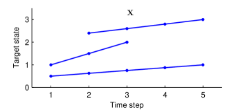
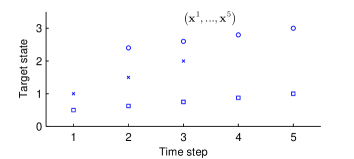
Figure 2: Illustration of set of trajectories of Example 1 (top) and an equivalent sequence of sets of labelled targets where squares, crosses and circles represent three different labels (bottom).

II-B Motivation for sets of trajectories

In this section, we motivate the importance of considering the multitrajectory density, defined over sets of trajectories, in a full Bayesian approach to MTT.

In vector based state space models, it is often important to consider the posterior density over the state trajectory, which contains the states at all time steps, i.e., it is not sufficient to merely find all the marginal densities of the states at all times [31, 32]. For example, the posterior density over the trajectory is necessary to calculate the maximum a posterior (MAP) estimator of the trajectory [33] or to answer trajectory-related questions, e.g., what is the probability that the state was in a region at a time and has moved to another region at a different time step?

The same is true in MTT. Sometimes, it is not sufficient to calculate multitarget densities at all time steps, we need a multitrajectory density as it enables us to answer all trajectory related questions, see Figure 1. For example, what is the probability that a target was in Madrid four hours ago and is currently in Gothenburg? This problem of defining a multitrajectory density to answer trajectory related questions has received little attention in the MTT literature and, in this section, we present arguments that support the idea that such a multitrajectory density should be defined on the space of sets of trajectories. To this end, we proceed to review some characteristics of labelled RFS approaches to MTT and indicate their shortcomings.

In the typical labelled RFS approach, we consider the sequence of multitarget densities on the set of labelled targets up to the current time step, which can be used to estimate suitable trajectories in many situations. However, this sequence of multitarget densities does not contain all available information and does not let us answer trajectory related questions, which are of key importance in tracking. As we illustrate next, a lack of complete information is particularly problematic when there is an unknown association between (unlabelled) targets states and labels. Two examples when this happens is when the birth process is an IID cluster RFS, in which the new born targets are IID given the cardinality [12, Sec. 4.3.2], and when targets get in close proximity and then separate [34, 35, 36]. This is an important weakness since the Poisson RFS, a specific type of IID cluster RFS, is a commonly used birth model [8, Sec. 14.2.1][24]. We illustrate the problem of the IID cluster birth RFS in a simple example.

Example 2.

Let us consider the following scenario. New born targets at time 1 are modelled by a labelled multi-Bernoulli RFS with two components. According to the labelling convention in [17, Sec. IV.D], the labels of the two components are $a=\left(1,1\right)$ and $b=\left(1,2\right)$, where the first component of the label is the time of birth and the second, a unique index to distinguish targets born at the same time. Both components have existence probability one and the same Gaussian density with a certain mean and variance. Note that if we remove the labels, the new born targets are an IID cluster RFS. Targets move independently with a given transition density and probability of survival one and no more targets can be born afterwards. Target states (without labels) are observed directly using the standard measurement model with no clutter, probability of detection 1 and negligible noise [12]. This implies that, at each time $k\in\left\{1,...,5\right\}$, the measurement set is $\left\{z_{1}^{k},z_{2}^{k}\right\}=\left\{x_{1}^{k},x_{2}^{k}\right\}$, where $\left\{x_{1}^{k},x_{2}^{k}\right\}$ is the set of unlabelled targets at time step $k$. We also assume that the single target transition density is such that target movements from $z_{1}^{k-1}$ to $z_{2}^{k}$ and from $z_{2}^{k-1}$ to $z_{1}^{k}$ do not occur. We have described a toy example without uncertainties in the two trajectories, but, as we will see, it is still challenging to handle using labelled multitarget densities.

The labelled multitarget filtering density $\pi^{k}\left(\cdot\right)$ at time $k$, which is given by the $\delta$-generalised labelled multi-Bernoulli ($\delta$-GLMB) filter [17] and coincides with the smoothing solution, is

$$\pi^{k}\left(\left\{\left(x_{1}^{k},l_{1}^{k}\right),\left(x_{2}^{k},l_{2}^{k}\right)\right\}\right)$$

$$=\frac{1}{2}\left(\delta_{z_{1}^{k}}\left(x_{1}^{k}\right)\delta_{z_{2}^{k}}\left(x_{2}^{k}\right)+\delta_{z_{1}^{k}}\left(x_{2}^{k}\right)\delta_{z_{2}^{k}}\left(x_{1}^{k}\right)\right)$$

$$\quad\times\left(\delta_{a}\left[l_{1}^{k}\right]\delta_{b}\left[l_{2}^{k}\right]+\delta_{a}\left[l_{2}^{k}\right]\delta_{b}\left[l_{1}^{k}\right]\right)$$ (2)

and zero for other sets of labelled targets. Notation $\delta_{y}\left(\cdot\right)$ and $\delta_{y}\left[\cdot\right]$ represent the Dirac and Kronecker delta centered at $y$, respectively, and $\left(x_{j}^{k},l_{j}^{k}\right)$ represents the state and label of target $j$ at time $k$. Evidently, the multitarget filtering/smoothing density at any time $k$ contains the information that there are targets located at $\left\{z_{1}^{k},z_{2}^{k}\right\}$, but labelling them as $\left\{\left(z_{1}^{k},a\right),\left(z_{2}^{k},b\right)\right\}$ is as likely as $\left\{\left(z_{1}^{k},b\right),\left(z_{2}^{k},a\right)\right\}$. This result holds even though the transition density indicates that movements from $z_{1}^{k-1}$ to $z_{2}^{k}$ and from $z_{2}^{k-1}$ to $z_{1}^{k}$ do not happen. Therefore, if we follow the usual procedure and build possible trajectories by linking target states and labels by using the filtering/smoothing multitarget densities in isolation, we obtain many possible sequences $\left(\mathbf{x}^{1},...,\mathbf{x}^{5}\right)$ of labelled sets, which represent trajectories. For example, as illustrated in Figure 3, we can have $\mathbf{x}^{k}=\left\{\left(a,z_{1}^{k}\right),\left(b,z_{2}^{k}\right)\right\}$ for all $k$, see Figure 3(a), but also $\mathbf{x}^{k}=\left\{\left(a,z_{1}^{k}\right),\left(b,z_{2}^{k}\right)\right\}$ for odd $k$ and $\mathbf{x}^{k}=\left\{\left(b,z_{1}^{k}\right),\left(a,z_{2}^{k}\right)\right\}$ for even $k$, see Figure 3(b). Consequently, we cannot tell how targets move between different time steps.

We recall that the total ambiguity in label-to-target associations in this example happens due to the type of birth model and the use of multitarget filtering/smoothing densities. Therefore, in this case, estimators based on these densities do not have enough information to link the target states and form suitable trajectories. In practice, one can employ pragmatic fixes, which can also be used with unlabelled filters [24], to estimate sensible trajectories in this example. For instance, one can use the dynamic model or the metadata associated to the filters, such as the history of data associations. Nevertheless, a full Bayesian methodology to MTT should not rely on pragmatic fixes, but on densities that contain the required information. $\oblong$

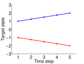
(a)

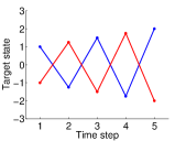
(b)

Figure 3: Illustration of two possible trajectory states from the sequence of labelled multitarget filtering/smoothing densities of Example 2. If we use the multitrajectory filtering density (defined on the space of sets of trajectories), the only possible state is the one in the left figure.

The previous issues of performing MTT using labelled multitarget densities can be solved by considering the joint density over the sequence of sets of labelled targets [25]. This density contains full trajectory information so it enables us to answer all trajectory-related questions. However, this representation has two drawbacks. The first one is that, due to the inclusion of arbitrary labels, this sequence of sets of labelled targets does not uniquely represent the underlying physical reality, see Example 1. This implies that we cannot define metrics with physical interpretation, on the space of sequences of sets of labelled targets, because, due to the identity property of metrics [13], we always obtain a non-zero distance/error between two different sequences of sets of labelled targets describing the same trajectories. For instance, changing the crosses and circles in Figure 2(bottom), we represent the same trajectories but the distance between this sequence of labelled sets and the (equivalent) original one is non-zero for any metric on the space of sequences of sets of labelled targets. This means that evaluating the performance of MTT algorithms using a metric on the space of sequences of sets of labelled targets is not useful, as it can provide a non-zero distance/error when there is no estimation error. The second drawback is that the explicit expressions of the joint densities over the sequence of labelled targets are cumbersome, as is illustrated in the next example.

Example 3.

The joint density over the sequence of labelled sets for the first two time steps in the scenario described in Example 2 is explicitly written as [18]

$$\pi^{1:2}\left(\left\{\left(x_{1}^{1},l_{1}^{1}\right),\left(x_{2}^{1},l_{2}^{1}\right)\right\},\left\{\left(x_{1}^{2},l_{1}^{2}\right),\left(x_{2}^{2},l_{2}^{2}\right)\right\}\right)$$

$$=\frac{1}{2}\left[\left(\delta_{\left(a,b,a,b\right)}\left[l_{1}^{1},l_{2}^{1},l_{1}^{2},l_{2}^{2}\right]+\delta_{\left(a,b,a,b\right)}\left[l_{2}^{1},l_{1}^{1},l_{2}^{2},l_{1}^{2}\right]\right)\right.$$

$$\times\left(\delta_{\left(z_{1}^{1},z_{2}^{1},z_{1}^{2},z_{2}^{2}\right)}\left(x_{1:2}^{1:2}\right)+\delta_{\left(z_{2}^{1},z_{1}^{1},z_{2}^{2},z_{1}^{2}\right)}\left(x_{1:2}^{1:2}\right)\right)$$

$$+\left(\delta_{\left(a,b,a,b\right)}\left[l_{1}^{1},l_{2}^{1},l_{2}^{2},l_{1}^{2}\right]+\delta_{\left(a,b,a,b\right)}\left[l_{2}^{1},l_{1}^{1},l_{1}^{2},l_{2}^{2}\right]\right)$$

$$\left.\times\left(\delta_{\left(z_{2}^{1},z_{1}^{1},z_{1}^{2},z_{2}^{2}\right)}\left(x_{1:2}^{1:2}\right)+\delta_{\left(z_{1}^{1},z_{2}^{1},z_{2}^{2},z_{1}^{2}\right)}\left(x_{1:2}^{1:2}\right)\right)\right]$$

where $x_{1:2}^{1:2}$ is used in this example to denote $\left(x_{1}^{1},x_{2}^{1},x_{1}^{2},x_{2}^{2}\right)$ and $\pi^{1:2}\left(\cdot\right)$ is zero for other sequences of labelled sets. As required, according to this density, $z_{1}^{1}$ and $z_{2}^{1}$ can only be linked with $z_{1}^{2}$ and $z_{2}^{2}$, respectively. However, these links arise in multiple combinations of the sequence of labelled sets $\left(\left\{\left(x_{1}^{1},l_{1}^{1}\right),\left(x_{2}^{1},l_{2}^{1}\right)\right\},\left\{\left(x_{1}^{2},l_{1}^{2}\right),\left(x_{2}^{2},l_{2}^{2}\right)\right\}\right)$. In fact, for a sequence of length $k$, in this example we have that the number of terms in the joint density is $2^{k+1}$, which represents the number of possible associations of target states to measurements ($2^{k}$) and 2 possible ways of labelling them. Even though we only consider two time steps, the above expression already contains 8 terms and the corresponding expression for a sequence of length five contains 64 terms. Due to this exponential increase in the number of terms, the inclusion of labels makes the explicit expression cumbersome even for relatively short sequences. $\oblong$

The mentioned drawbacks of sequences of labelled sets can be solved by using sets of trajectories. Sets of trajectories do not include arbitrary parameters so we can develop metrics, such as the ones proposed in [26, 27]. Though these metrics are not metrics on the space of sequences of sets of labelled targets, they can be used to evaluate MTT algorithms based on sequences of sets of labelled targets, by representing the resulting estimates in terms of sets of (unlabelled) trajectories. In addition, a (multiobject) density on the set of trajectories enables us to answer all possible trajectory related questions with a more compact representation, as illustrated in the next example.

Example 4.

As we will explain in this paper, by applying Mahler’s RFS framework to set of trajectories, the multitrajectory density for the five time steps in Example 2 is

$$\pi^{5}\left(\left\{\left(t_{1},x_{1}^{1:i_{1}}\right),\left(t_{2},x_{2}^{1:i_{2}}\right)\right\}\right)$$

$$=\left(\delta_{z_{1}^{1:5}}\left(x_{1}^{1:i_{1}}\right)\delta_{z_{2}^{1:5}}\left(x_{2}^{1:i_{1}}\right)+\delta_{z_{1}^{1:5}}\left(x_{2}^{1:i_{1}}\right)\delta_{z_{2}^{1:5}}\left(x_{1}^{1:i_{1}}\right)\right)$$

$$\quad\times\delta_{1}\left[t_{1}\right]\delta_{1}\left[t_{2}\right]\delta_{5}\left[i_{1}\right]\delta_{5}\left[i_{2}\right],$$

and zero for other sets of trajectories. This multitrajectory density has complete trajectory information with a significant decrease in the number of terms compared to the joint density over the sequence of labelled sets, 2 terms versus 64, as pointed out in Example 3. $\oblong$

Once the full Bayesian problem is properly characterised, we can develop algorithms/approximations to handle the trajectory-related questions of the application at hand. For example, if our application only requires us to estimate the number of targets and their positions at the current time, it is enough to consider the filtering multitarget density at the current time, as in the usual RFS approach.

II-C Probability and integration

In this paper, probability and integration are defined using finite set statistics (FISST) [8, 12], which is related to measure theory [37]. Even though FISST usually considers sets of targets, it can be applied to sets of trajectories by changing the single object state (targets by trajectories) and single object integrals (single target integrals by single trajectory integrals). In Appendix A, we explain why we can use FISST with sets of trajectories and how to obtain the corresponding single-trajectory integrals and set integrals, which are given in the following.

Given a real-valued function $\pi\left(\cdot\right)$ on the single trajectory space $T_{\left(k^{\prime}\right)}$, its integral is

$$\int\pi\left(X\right)dX =\sum_{\left(t,i\right)\in I_{(k^{\prime})}}\int\pi\left(t,x^{1:i}\right)dx^{1:i}.$$ (3)

This integral goes through all possible start times, lengths and target states of the trajectory. Given a real-valued function $\pi\left(\cdot\right)$ on the space $\mathcal{F}\left(T_{\left(k^{\prime}\right)}\right)$ of sets of trajectories, its set integral is [8]:

$$\int\pi\left(\mathbf{X}\right)\delta\mathbf{X} =\sum_{n=0}^{\infty}\frac{1}{n!}\int\pi\left(\left\{X_{1},...,X_{n}\right\}\right)dX_{1:n}$$ (4)

where $X_{1:n}=\left(X_{1},...,X_{n}\right)$. Note that, if $\pi\left(\cdot\right)$ is a multitrajectory density, then, $\pi\left(\cdot\right)\geq 0$ and its set integral is one.

We can also use set integrals to calculate the probability that an RFS of trajectories belongs to a certain region. In order to do so, we define a mapping $\chi:\uplus_{n\text{=0}}^{\infty}T_{\left(k^{\prime}\right)}^{n}\rightarrow\mathcal{F}\left(T_{\left(k^{\prime}\right)}\right)$ of sequences of trajectories to sets of trajectories such that $\chi\left(\left(X_{1},...,X_{n}\right)\right)=\left\{X_{1},...,X_{n}\right\}$. Given a region $A=\uplus_{n\text{=0}}^{\infty}A_{n}$ where $A_{n}\subseteq\mathcal{F}\left(T_{\left(k^{\prime}\right)}\right)$ is a set that contains sets with $n$ elements in $T_{\left(k^{\prime}\right)}$, the probability that $\mathbf{X}$ belongs to $A$ is

$$P\left(\mathbf{X}\in A\right) =\sum_{n=0}^{\infty}\frac{1}{n!}\int_{\chi^{-1}\left(A_{n}\right)}\pi\left(\left\{X_{1},...,X_{n}\right\}\right)dX_{1:n}.$$ (5)

where $\pi\left(\cdot\right)$ is the multitrajectory density of $\mathbf{X}$. Equation (5) is proved in Appendix B. For instance, if $A_{2}=\left\{\left\{X_{1},X_{2}\right\}:X_{1}\in B_{1},X_{2}\in B_{2}\right\}$ where $B_{1}\subseteq T_{\left(k^{\prime}\right)}$ and $B_{2}\subseteq T_{\left(k^{\prime}\right)}$, then $\chi^{-1}\left(A_{2}\right)=\left\{\left(X_{1},X_{2}\right):X_{1}\in B_{1},X_{2}\in B_{2}\,\mathrm{or}\,X_{2}\in B_{1},X_{1}\in B_{2}\right\}$. Calculating (5) for $A_{2}$, we obtain the probability that there are two trajectories, one in region $B_{1}$ and another one in region $B_{2}$. Equation (5) is necessary to obtain certain probabilities of interest, for example, the probability that there is a number of trajectories present at a certain time instant or a number of targets in a given region at a given time. The cardinality distribution $\rho\left(\cdot\right)$ indicates the probability that $n$ trajectories have existed at all times

$$\rho\left(n\right) =P\left(\mathbf{X}\in\chi\left(T_{\left(k^{\prime}\right)}^{n}\right)\right)$$

$$=\frac{1}{n!}\int\pi\left(\left\{X_{1},...,X_{n}\right\}\right)dX_{1:n},$$ (6)

which is analogous for RFSs of targets [8, Eq. (11.115)].

Example 5.

We consider a multitrajectory density $\pi\left(\cdot\right)$ such that

$$\pi\left(\left\{\left(1,x_{1}^{1:2}\right)\right\}\right) =0.9\mathcal{N}\left(x_{1}^{1:2};\left(10,11\right),\left[\begin{array}[]{cc}1&1\\ 1&2\end{array}\right]\right)$$

$$\pi\left(\left\{\left(1,x_{1}^{1:2}\right),\left(2,x_{2}^{1}\right)\right\}\right) =0.1\mathcal{N}\left(x_{1}^{1:2};\left(10,11\right),\left[\begin{array}[]{cc}1&1\\ 1&2\end{array}\right]\right)$$

$$\quad\times\mathcal{N}\left(x_{2}^{1};100,1\right),$$

where $\mathcal{N}\left(\cdot;\overline{x},P\right)$ denotes a Gaussian density with mean $\overline{x}$ and covariance matrix $P$, and $\pi\left(\cdot\right)$ is zero for other sets of trajectories. From (6), we see that the probability that there is one trajectory is 0.9 and the probability for two trajectories is 0.1. The probability that there is only one trajectory and this trajectory starts at time step 1 in a region $B_{1}\subseteq D$ and moves to a region $B_{2}\subseteq D$ at the next time step can be obtained by integrating $\pi\left(\cdot\right)$ over the region $A_{1}=\chi\left(\left\{1\right\}\times B\times\uplus_{i=0}^{k^{\prime}-2}D^{i}\right)$, where $B=B_{1}\times B_{2}$. That is, region $A_{1}$ considers start time 1 with the first two states belonging to $B$. Then, the trajectory can die at any moment afterwards and, when it is present, its state at a particular time belongs to $D$. Then,

$$P\left(\mathbf{X}\in A_{1}\right) =0.9\int_{B}\mathcal{N}\left(x_{1}^{1:2};\left(10,11\right),\left[\begin{array}[]{cc}1&1\\ 1&2\end{array}\right]\right)dx_{1}^{1:2}$$ (9)

where we have used (5) and that $\chi^{-1}\left(A_{1}\right)=\left\{1\right\}\times B\times\uplus_{i=0}^{k^{\prime}-2}D^{i}$. Note that, using the notation in (5), $A=A_{1}$, as the integration region in this example only contains sets of cardinality $1$ and, therefore, (9) only considers the term that corresponds to $n=1$ in (5). $\oblong$

III Filtering recursion for RFSs of trajectories

In this section, we present the filtering recursion for RFS of trajectories. We first present the dynamic model of the trajectories in Section III-A. Then, for this dynamic model, we present the filtering recursion for a general measurement model and for the standard measurement model in Sections III-B and III-C, respectively. We discuss some practical considerations in Section III-D.

III-A Dynamic model

We consider the conventional assumptions for the dynamic model used in the RFS framework [8]:

• Given the current multitarget state ${\bf x}$, each target $x\in{\bf x}$ survives with probability $p_{S}\left(x\right)$ and moves to a new state with a transition density $g\left(\cdot\left|x\right.\right)$, or dies with probability $1-p_{S}\left(x\right)$.

• The multitarget state at the next time step is the union of the surviving targets and new targets, which are born independently of the rest with a multitarget density $\beta_{\tau}\left(\cdot\right)$.

In this paper, we use the subindex $\tau$ in multitarget densities to differentiate them from multitrajectory densities. The previous parameters of the dynamic model can change with time but we omit time dependence for notational simplicity. Note that, as in filtering RFS of targets, this model implies that the number of trajectories and new born targets at each time step is unknown. As we will see, this dynamic model gives rise to a transition multitrajectory density $f^{k}\left(\cdot\left|\cdot\right.\right)$ for the set of trajectories at time $k$, which includes all trajectories that have ever been present.

Example 6.

We proceed to illustrate how the set of trajectories of Example 1, which is represented in Figure 2, evolves with time. We consider that the current time step is $k=5$ and discuss what the set may look like at time $k=6$. Trajectory $X_{1}$, which is not present at time 5, remains unaltered. Trajectory $X_{2}$ survives with probability $p_{S}\left(1\right)$, which means that it becomes $X_{2}=\left(1,\left(0.5,0.625,0.75,0.875,1,y\right)\right)$ with $y\sim g\left(\cdot\left|1\right.\right)$, or remains unaltered with probability $1-p_{S}\left(1\right)$. An analogous behaviour is shown by $X_{3}$. The new set is guaranteed to contain these three trajectories plus new trajectories determined by the new born targets, generated from the birth process $\beta_{\tau}\left(\cdot\right)$, and the time of appearance $6$. For illustration, in Figure 4, we show 20 realisations of the random set of trajectories at time 6 using $g\left(y\left|x\right.\right)=\mathcal{N}\left(y;x,0.01\right)$, probability of survival one at time 5 ($p_{S}\left(\cdot\right)=1$), and no new born targets at time 6. $\oblong$

For this dynamic model, we present the filtering recursion for a general measurement model in Section III-B and for the standard measurement model in Section III-C.

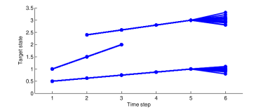
Figure 4: Dynamic model: 20 possible realisations of the random set of trajectories at time 6 given the set of trajectories of Figure 2 at time 5. No new born targets are considered and $p_{S}\left(\cdot\right)=1$.

III-B Filtering with a general measurement model

The set of targets at time $k$ is observed through noisy measurements giving rise to the likelihood $\ell^{k}\left(\cdot\right)$, where we omit the value of the measurement for notational simplicity [38]. By using FISST [12], the multitrajectory filtering density $\pi^{k}\left(\cdot\right)$ at time $k$, i.e., the multitrajectory density of the set of trajectories up to time step $k$ given the sequence of measurements up to time step $k$, can be calculated recursively using the prediction and update equations,

$$\pi^{k|k-1}\left(\mathbf{X}\right) =\int f^{k}\left(\mathbf{X}\left|\mathbf{Y}\right.\right)\pi^{k-1}\left(\mathbf{Y}\right)\delta\mathbf{Y}$$ (10)

$$\pi^{k}\left(\mathbf{X}\right) \propto\ell^{k}\left(\mathbf{X}\right)\pi^{k|k-1}\left(\mathbf{X}\right).$$ (11)

Here, $\propto$ means “is proportional to” and $\pi^{k|k-1}\left(\cdot\right)$ is referred to as the predicted multitrajectory density at time $k$, which represents the density of the set of trajectories at time $k$ given the sequence of measurements up to time $k-1$. It should be noted that $\mathbf{X}$ drawn from $\pi^{k}\left(\cdot\right)$ or $\pi^{k|k-1}\left(\cdot\right)$ is a set of trajectories in the time interval 1 to $k$. That is, we have that $\pi^{k}\left(\mathbf{X}\right)=0$ and $\pi^{k|k-1}\left(\mathbf{X}\right)=0$ if $\mathbf{X}$ contains a trajectory that is present at a time step that is higher than $k$. After time $k$, some trajectories in $\mathbf{X}$ may be extended, as illustrated in Figure 4, and new trajectories may appear. These properties imply that we only need to compute the set integrals up to time step $k$. In theory, set integrals are defined up to some finite time step $k\text{\textquoteright}$, see (3), but, as long as $k\text{\textquoteright}>k$, the actual value of $k\text{\textquoteright}$ is irrelevant and does not have to be specified.

For general track-before-detect measurement models, the likelihood $\ell^{k}\left(\cdot\right)$ cannot be simplified so we just write the update as in (11) [38]. The following theorem indicates how to evaluate the prediction (10) more explicitly.

Theorem 7.

We consider the conventional dynamic model, which includes the functions $p_{S}\left(\cdot\right)$, $g\left(\cdot\left|\cdot\right.\right)$ and $\beta_{\tau}\left(\cdot\right)$, explained at the beginning of Section III-A, and trajectories up to time step $k$. Then, given a set $\mathbf{W}$ of new born trajectories at time $k$, a set $\mathbf{X}$ of trajectories present at times $k-1$ and $k$, a set $\mathbf{Y}$ of trajectories present at time $k-1$ but not present at time $k$ and a set $\mathbf{Z}$ of trajectories present at a time before $k-1$ but not at $k-1$, the predicted multitrajectory density $\pi^{k|k-1}\left(\cdot\right)$ at time $k$ is

$$\pi^{k|k-1}\left(\mathbf{W}\uplus\mathbf{X}\uplus\mathbf{Y}\uplus\mathbf{Z}\right)$$

$$=\prod_{\left(t,x^{1:i}\right)\in\mathbf{X}}\left(g\left(x^{i}\left|x^{i-1}\right.\right)p_{S}\left(x^{i-1}\right)\right)\prod_{\left(t,x^{1:i}\right)\in\mathbf{Y}}\left(1-p_{S}\left(x^{i}\right)\right)$$

$$\quad\times\pi^{k-1}\left(\cup_{\left(t,x^{1:i}\right)\in\mathbf{X}}\left\{\left(t,x^{1:i-1}\right)\right\}\uplus\mathbf{Y}\uplus\mathbf{Z}\right)\beta_{\tau}\left(\tau^{k}\left(\mathbf{W}\right)\right).$$

Theorem 7 is proved in Appendix C. We first clarify that if $\left(t,x^{1:i}\right)\in\mathbf{W}$, then, $t=k$, $i=1$; if it belongs to $\mathbf{X}$, then $t<k$, $i=k-t+1$; if it belongs to $\mathbf{Y}$, then $t<k$, $i=k-t$; and finally, if it belongs to $\mathbf{Z}$, then, $t<k-1$, $i<k-t$. To evaluate the predicted multitrajectory density at time $k$, we multiply the following terms: multitrajectory filtering density $\pi^{k-1}\left(\cdot\right)$ for trajectories present at previous times, $g\left(\cdot|\cdot\right)$ and $p_{S}\left(\cdot\right)$ for surviving trajectories, $\left(1-p_{S}\left(\cdot\right)\right)$ for trajectories present at time $k-1$ but not present at $k$ and the multitarget density $\beta_{\tau}\left(\cdot\right)$ for new born targets.

III-C Filtering with the standard measurement model

In this section, we present the following key result: for the standard (point target) measurement model (12) and the birth model (16), the multitrajectory filtering and predicted densities at all time steps have the same form, which is a multi-Bernoulli mixture in which the existence probabilities are either 0 or 1, which we refer to as $\mathrm{MBM}_{01}$ [39, Sec. IV]. Therefore, the $\mathrm{MBM}_{01}$ multitrajectory density is conjugate with respect to the standard measurement likelihood [17]. How to obtain these multitrajectory densities recursively is indicated by Lemmas 9 and 10, which give rise to the trajectory $\mathrm{MBM}_{01}$ filter. We use the multiobject exponential notation $h^{\mathbf{x}}=\prod_{x\in\mathbf{x}}h\left(x\right)$ where $h$ is a real-valued function and $h^{\emptyset}=1$ by convention [17].

The standard measurement model [12] is described as:

• For a given multi-target state $\mathbf{x}$ at time $k$, each target state $x\in\mathbf{x}$ is either detected with probability $p_{D}\left(x\right)$ and generates one measurement with density $l\left(\cdot|x\right)$, or missed with probability $1-p_{D}\left(x\right)$.

• The measurement set $\mathbf{z}^{k}$ is the union of the target-generated measurements and Poisson clutter with intensity function $\kappa\left(\cdot\right)$.

We proceed to write the resulting likelihood [12, Eq. (7.21)] in terms of sets of trajectories in a form that will be useful in the rest of the section.

Given a set $\mathbf{X}\uplus\mathbf{Y}$ of trajectories such that $\mathbf{X}=\left\{X_{1},...,X_{n}\right\}$ with $n$ present trajectories at time $k$ and a set $\mathbf{Y}$ of trajectories with no present trajectories at time $k$, the measurement set $\mathbf{z}^{k}=\left\{z_{1}^{k},...,z_{m}^{k}\right\}$ only depends on $\tau^{k}\left(\mathbf{X}\right)$ as explained before. Then, the likelihood at time $k$ for the standard measurement model is

$$\ell^{k}\left(\mathbf{X}\uplus\mathbf{Y}\right) =e^{-\int\kappa\left(z\right)dz}\kappa^{\mathbf{z}^{k}}\sum_{\theta\in\Theta_{n,m}}\prod_{j=1}^{n}\psi_{\mathbf{z}^{k}}\left(X_{j}|\theta_{j}\right),$$ (12)

where $\Theta_{n,m}$ denotes all data association hypotheses for $n$ targets (which correspond to $n$ present trajectories) and $m$ measurements. More specifically, for $\theta=\left(\theta_{1},...,\theta_{n}\right)\in\Theta_{n,m}$, $\theta_{i}=j$ if the $i$th present target is associated with the $j$th measurement or $0$ if it is undetected. Due to the properties of the standard measurement model, we have that, if $\theta_{i}=\theta_{j}>0$, then $i=j$. Also,

$$\psi_{\mathbf{z}^{k}}\left(t,x^{1:i}|\theta_{j}\right) =\left\{\begin{array}[]{cc}\frac{p_{D}\left(x^{k-t+1}\right)l\left(z_{\theta_{j}}^{k}|x^{k-t+1}\right)}{\kappa\left(z_{\theta_{j}}^{k}\right)}&\theta_{j}>0\\ 1-p_{D}\left(x^{k-t+1}\right)&\theta_{j}=0,\end{array}\right.$$ (15)

where $x^{k-t+1}$ is the state of trajectory $\left(t,x^{1:i}\right)$ that corresponds to time step $k$. If $\mathbf{X}=\emptyset$, then $\ell^{k}\left(\mathbf{Y}\right)=e^{-\int\kappa\left(z\right)dz}\kappa^{\mathbf{z}^{k}}$.

In order to obtain the explicit recursion, we assume that the targets can be born from $b$ densities $\beta_{1}\left(\cdot\right)$, …, $\beta_{b}\left(\cdot\right)$ with a weight $w_{B}\left(L\right):\,L\subseteq\mathbb{N}_{b}$, which indicates the probability that $\left|L\right|$ targets are born from the densities indicated by $L$. The resulting multitarget density for new born targets is

$$\beta_{\tau}\left(\left\{x_{1},...,x_{n}\right\}\right) =\sum_{l_{1:n}}^{\neq}w_{B}\left(\left\{l_{1},...,l_{n}\right\}\right)\prod_{j=1}^{n}\beta_{l_{j}}\left(x_{j}\right),$$ (16)

where $n\leq b$ and the sum is performed over distinct elements:

$$\sum_{l_{1:n}}^{\neq} =\sum_{l_{1:n}:l_{1}\neq...\neq l_{n}}.$$

The birth model in (16) corresponds to an $\mathrm{MBM}_{01}$, see Appendix D. Note that we can draw samples from (16) by first generating the auxiliary set $L$, whose cardinality is the number of new born targets, from $w_{B}\left(\cdot\right)$ and then drawing the target states from the corresponding densities independently.

Example 8.

Let us consider one-dimensional targets that are born according to the model (16) with $b=2$,

$$\beta_{i}\left(x\right) =\mathcal{N}\left(x;\mu_{i},\sigma_{i}^{2}\right)$$

where $\mu_{i}$ and $\sigma_{i}^{2}$ represent the mean and variance of the $i$th birth component, $w_{B}\left(\emptyset\right)=0.8$, $w_{B}\left(\left\{1\right\}\right)=0.1$, $w_{B}\left(\left\{2\right\}\right)=0.05$ and $w_{B}\left(\left\{1,2\right\}\right)=0.05$. This means that no target is born with probability 0.8, one target is born from density $\beta_{1}\left(\cdot\right)$ with probability 0.1 and from $\beta_{2}\left(\cdot\right)$ with probability 0.05. Finally, two targets are born with probability 0.05, one from density $\beta_{1}\left(\cdot\right)$ and another from $\beta_{2}\left(\cdot\right)$. $\oblong$

If the likelihood is (12) and the multitarget density of new born targets is (16), we show in this section that the multitrajectory filtering density can be written as

$$\pi^{k}\left(\left\{X_{1},...,X_{n}\right\}\right) =\sum_{h_{1:n}^{k|k}}^{\neq}w^{k|k}\left(\left\{h_{1}^{k|k},...,h_{n}^{k|k}\right\}\right)$$

$$\quad\times\prod_{j=1}^{n}p^{k|k}\left(X_{j}|h_{j}^{k|k}\right)$$ (17)

where $h_{j}^{k|k}=\left(l_{j},t_{j},i_{j},\xi_{j}\right)$ is a single trajectory hypothesis which implies that the density $p^{k|k}\left(\cdot|h_{j}^{k|k}\right)$ (on $T_{\left(k^{\prime}\right)}$) has been obtained by propagating birth component $\beta_{l_{j}}\left(\cdot\right)$ with starting time $t_{j}$, duration $i_{j}$ and data associations $\xi_{j}$. Here, $\xi_{j}$ is a vector of length $i_{j}$ that takes values 0 if the density $p^{k|k}\left(\cdot|h_{j}^{k|k}\right)$ is associated with clutter or $i$ if it is associated with the $i$th measurement at the corresponding time step. The sum in (17) goes over over all trajectory hypotheses that may occur jointly up to the current time. As the birth model (16), this multitrajectory density is also an $\mathrm{MBM}_{01}$. We can see that hypothesis $h_{j}^{k|k}$ includes the pair $\left(l_{j},t_{j}\right)$, which corresponds to the label in [17], but the label is not included in the trajectory state. More details about the labelled approach are given in Section IV-A.

We also show that the multitrajectory predicted density at time $k$ has the same form as (17) and can be written as

$$\pi^{k|k-1}\left(\left\{X_{1},...,X_{n}\right\}\right) =\sum_{h_{1:n}^{k|k-1}}^{\neq}w^{k|k-1}\left(\left\{h_{1}^{k|k-1},...,h_{n}^{k|k-1}\right\}\right)$$

$$\quad\times\prod_{j=1}^{n}p^{k|k-1}\left(X_{j}|h_{j}^{k|k-1}\right)$$ (18)

where $h_{j}^{k|k-1}$ is the same as $h_{j}^{k|k}$ but the data association vector has $i_{j}-1$ components as the data association at time $k$ has not been done yet. The resulting steps of the trajectory $\mathrm{MBM}_{01}$ filtering recursion, which are explained in the rest of the section, are shown in Procedure 1. As we consider that trajectories cannot be born before time step 1, see Section II-A, we can set $w^{0|0}\left(\emptyset\right)=1$ such that trajectories at time 1 are born according to the birth model. In addition, $w^{0|0}\left(\emptyset\right)=1$ is a particular case of (17) so the multitrajectory $\mathrm{MBM}_{01}$ density is conjugate for the standard model.

Procedure 1 Steps of the trajectory $\mathrm{MBM}_{01}$ filter

- Initialisation: $w^{0|0}\left(\emptyset\right)=1$.

for  $k=1$ to final time step  do

     - Prediction: Generate the new hypothesis sets and calculate/approximate their weights $w^{k|k-1}\left(\cdot\right)$ and trajectory densities $p^{k|k-1}\left(\cdot|\cdot\right)$ using Lemma 9.

     - Update: Generate the new hypothesis sets and calculate/approximate their weights $w^{k|k}\left(\cdot\right)$ and trajectory densities $p^{k|k}\left(\cdot|\cdot\right)$ using Lemma 10.

end for

Before providing the recursive formulas for computing (17) and (18), we introduce the following sets of single trajectory hypotheses $\left(l,t,i,\xi\right)$: $\mathbb{U}^{k}$ contains the hypotheses of a present trajectory at time $k$ that has a data association hypothesis at time $k$; $\mathbb{S}^{k}$ contains the hypotheses of a surviving trajectory at time $k$ that does not yet contain a data association hypothesis at time $k$, $\mathbb{D}^{k}$ contains the hypotheses of trajectories present at time $k-1$ but not present at time $k$, $\mathbb{N}^{k}$ contains the hypotheses of new born trajectories at time $k$ and $\mathbb{D}^{1:k}=\uplus_{j=1}^{k}\mathbb{D}^{j}$, which considers trajectories that ended at time $k-1$ or earlier. After the $k$th update step, a single trajectory hypothesis is contained in $\mathbb{U}^{k}\uplus\mathbb{D}^{1:k}$. Before the $k$th update step, a single trajectory hypothesis is contained in $\mathbb{S}^{k}\uplus\mathbb{N}^{k}\uplus\mathbb{D}^{1:k}$. Mathematically, these sets are given by

$$\mathbb{U}^{k} =\left\{\left(l,t,i,\xi\right):l\in\mathbb{N}_{b},t\leq k,t+i-1=k,\mathrm{d}\left(\xi\right)=i\right\}$$

$$\mathbb{S}^{k} =\left\{\left(l,t,i,\xi\right):l\in\mathbb{N}_{b},t<k,t+i-1=k,\mathrm{d}\left(\xi\right)=i-1\right\}$$

$$\mathbb{D}^{k} =\left\{\left(l,t,i,\xi\right):l\in\mathbb{N}_{b},t<k,t+i=k,\mathrm{d}\left(\xi\right)=i\right\}$$

$$\mathbb{N}^{k} =\left\{\left(l,k,1\right):l\in\mathbb{N}_{b}\right\}$$

where $\mathrm{d}\left(\xi\right)$ denotes the dimension of vector $\xi$.

Lemma 9 (Prediction).

Given $\pi^{k-1}\left(\cdot\right)$ of the form (17) and hypothesis sets $\mathcal{A}\subset\mathbb{S}^{k}$, $\mathcal{B}\subset\mathbb{D}^{k}$, $\mathcal{C}\subset\mathbb{N}^{k}$ and $\mathcal{D}\subset\mathbb{D}^{1:k-1}$, the predicted weight in (18) for the hypothesis set $\mathcal{A}\uplus\mathcal{B}\uplus\mathcal{C}\uplus\mathcal{D}$ is

$$w^{k|k-1}\left(\mathcal{A}\uplus\mathcal{B}\uplus\mathcal{C}\uplus\mathcal{D}\right)$$

$$\quad=\left[\gamma_{S}\right]^{\mathcal{A}}\left[\gamma_{D}\right]^{\mathcal{B}}w_{B}^{k}\left(\mathcal{C}\right)w^{k-1|k-1}\left(\mathcal{A}^{-}\uplus\mathcal{B}\uplus\mathcal{D}\right)$$ (19)

$$\gamma_{S}\left(h\right) =\int p_{S}\left(X^{|}\right)p^{k-1|k-1}\left(X|h^{-}\right)dX$$ (20)

$$\gamma_{D}\left(h\right) =1-\gamma_{S}\left(h\right)$$ (21)

$$w_{B}^{k}\left(\left\{\left(l_{1},k,1\right),...,\left(l_{n},k,1\right)\right\}\right) =w_{B}\left(\left\{l_{1},...,l_{n}\right\}\right)$$ (22)

where for $h=\left(l,t,i,\xi\right)$, we have $h^{-}=\left(l,t,i-1,\xi\right)$, $\mathcal{A}^{-}=\left\{h^{-}:h\in\mathcal{A}\right\}$ and $X^{|}$ is the last target state of $X$. Also, $w_{B}^{k}\left(\cdot\right)$ is zero if evaluated at global hypotheses different from (22).

The single trajectory density for $h\in\mathbb{S}^{k}\uplus\mathbb{D}^{k}\uplus\mathbb{N}^{k}\uplus\mathbb{D}^{1:k-1}$ is

$$p^{k|k-1}\left(X|h\right)$$

$$=p_{S}^{k|k-1}\left(X|h\right)1_{\mathbb{S}^{k}}\left(h\right)+p_{D}^{k|k-1}\left(X|h\right)1_{\mathbb{D}^{k}}\left(h\right)$$

$$\quad+p_{N}^{k|k-1}\left(X|h\right)1_{\mathbb{N}^{k}}\left(h\right)+p^{k-1|k-1}\left(X|h\right)1_{\mathbb{D}^{1:k-1}}\left(h\right)$$ (23)

where

$$p_{S}^{k|k-1}\left(t,x^{1:i}|h\right) =g\left(x^{i}|x^{i-1}\right)p_{S}\left(x^{i-1}\right)$$

$$\quad\times p^{k-1|k-1}\left(t,x^{1:i-1}|h^{-}\right)/\gamma_{S}\left(h\right)$$

$$p_{D}^{k|k-1}\left(t,x^{1:i}|h\right) =\frac{p^{k-1|k-1}\left(t,x^{1:i}|h\right)\left(1-p_{S}\left(x^{i}\right)\right)}{\gamma_{D}\left(h\right)}$$

$$p_{N}^{k|k-1}\left(t,x^{1}|l,k,1\right) =\beta_{l}\left(x^{1}\right)\delta_{k}\left[t\right].$$

This lemma is proved in Appendix D. Each hypothesis set in (19) can be decomposed into disjoint hypothesis sets $\mathcal{A}$, $\mathcal{B}$, $\mathcal{C}$ and $\mathcal{D}$ that describe surviving trajectories, present trajectories at time $k-1$ but not at time $k$, new born trajectories and trajectories that were present some time before time $k-1$ but not at time $k-1$, respectively. The weight $w^{k|k-1}\left(\cdot\right)$ corresponds to the weight $w^{k-1|k-1}\left(\cdot\right)$ of the parent hypothesis set $\mathcal{A}^{-}\uplus\mathcal{B}\uplus\mathcal{D}$ multiplied by the weight of the hypothesis set $\mathcal{C}$ of new born targets, the probability (20) of survival for trajectories hypothesised in $\mathcal{A}$ and the probability (21) of death for trajectories hypothesised in $\mathcal{B}$. The resulting density of a trajectory given a hypothesis is given by (23). Densities $p_{S}^{k|k-1}\left(\cdot|h\right)$, $p_{D}^{k|k-1}\left(\cdot|h\right)$ and $p_{N}^{k|k-1}\left(\cdot|h\right)$ correspond to a surviving trajectory, a trajectory present at time $k-1$ but not at time $k$, and a new born trajectory, respectively. If the trajectory is not present at time $k-1$, which means that its hypothesis is contained in $\mathbb{D}^{1:k-1}$, its density remains unaltered.

Lemma 10 (Update).

Given $\pi^{k|k-1}\left(\cdot\right)$ of the form (18), the measurement set $\mathbf{z}^{k}=\left\{z_{1}^{k},...,z_{m}^{k}\right\}$ and hypothesis sets $\mathcal{D}\subset\mathbb{D}^{1:k}$ and $\mathcal{E}=\left\{h_{1}^{k|k},...,h_{n}^{k|k}\right\}\subset\mathbb{U}^{k}$ such that $h_{j}^{k|k}=\left(h_{j}^{k|k-1},\theta_{j}\right)$, $\left(\theta_{1},...,\theta_{n}\right)\in\Theta_{n,m}$, the filtering weight in (17) for hypothesis set $\mathcal{E}\uplus\mathcal{D}$ is

$$w^{k|k}\left(\mathcal{E}\uplus\mathcal{D}\right) \propto w^{k|k-1}\left(\mathcal{E}^{\circ}\uplus\mathcal{D}\right)\left[\eta_{\mathbf{z}^{k}}\right]^{\mathcal{E}}$$ (24)

$$\eta_{\mathbf{z}^{k}}\left(h_{j}^{k|k-1},\theta_{j}\right) =\int\psi_{\mathbf{z}^{k}}\left(X|\theta_{j}\right)p^{k|k-1}\left(X|h_{j}^{k|k-1}\right)dX$$ (25)

where $\mathcal{E}^{\circ}=\left\{h_{1}^{k|k-1},...,h_{n}^{k|k-1}\right\}$.

The single trajectory density for $h_{j}^{k|k}\in\mathbb{U}^{k}\uplus\mathbb{D}^{1:k}$ is

$$p^{k|k}\left(X|h_{j}^{k|k}\right) =p_{U}^{k|k}\left(X|h_{j}^{k|k}\right)1_{\mathbb{U}^{k}}\left(h_{j}^{k|k}\right)$$

$$\quad+p^{k|k-1}\left(X|h_{j}^{k|k}\right)1_{\mathbb{D}^{1:k}}\left(h_{j}^{k|k}\right)$$ (26)

$$p_{U}^{k|k}\left(X|h_{j}^{k|k-1},\theta_{j}\right) =\frac{\psi_{\mathbf{z}^{k}}\left(X|\theta_{j}\right)p^{k|k-1}\left(X|h_{j}^{k|k-1}\right)}{\eta_{\mathbf{z}^{k}}\left(h_{j}^{k|k-1},\theta_{j}\right)}.$$

This lemma is proved in Appendix D. A hypothesis set in (24) can be decomposed into disjoint hypothesis sets $\mathcal{E}\uplus\mathcal{D}$ that describe present trajectories at time $k$ (with a data association hypothesis at time $k$) and trajectories that were present before time $k$ but not at time $k$, respectively. The weight $w^{k|k}\left(\cdot\right)$ corresponds to the weight $w^{k|k-1}\left(\cdot\right)$ of the parent hypothesis $\mathcal{E}^{\circ}\uplus\mathcal{D}$ multiplied by the data association probabilities $\eta_{\mathbf{z}^{k}}\left(\cdot\right)$ of the present trajectories. The resulting density of a trajectory for a hypothesis is given by (26). Density $p_{U}^{k|k}\left(\cdot|h_{j}^{k|k}\right)$ corresponds to a present trajectory at time $k$. If the trajectory is not present at time $k$, which means that its hypothesis is contained in $\mathbb{D}^{1:k}$, its density remains unaltered.

In the trajectory $\mathrm{MBM}_{01}$ filter, it is important to highlight that the update and prediction of the weights only depend on the densities of the target states at the current time. In other words, $\gamma_{S}\left(\cdot\right)$, $\gamma_{D}\left(\cdot\right)$ and $\eta_{\mathbf{z}^{k}}\left(\cdot\right)$ are calculated/approximated using a single target integral w.r.t. the density of the target $\tau^{k}\left(X\right)$ for the corresponding hypothesis. For linear/Gaussian dynamic and measurement models, with constant $p_{D}\left(\cdot\right)$ and $p_{S}\left(\cdot\right)$, and Gaussian $\beta_{i}\left(\cdot\right)$, Lemmas 9 and 10 can be implemented in closed-form, subject to the practical considerations of managing an ever-increasing number of hypotheses and trajectories, which are discussed in Section III-D. The resulting formulas can be found in Appendix E and are illustrated via simulations in Section V. If the system is nonlinear/non-Gaussian, we need to perform single trajectory density approximations to calculate (23) and (26).

We would also like to point out that there are three types of conjugate priors for unlabelled multi-target filtering in the literature, which depend on the birth model and the structure of the hypotheses [39, Sec. IV]: $\mathrm{MBM}_{01}$, multi-Bernoulli mixture (MBM), and Poisson multi-Bernoulli mixture (PMBM). This paper has introduced the $\mathrm{MBM}_{01}$ conjugate prior for sets of trajectories. Conjugacy for sets of trajectories also holds for PMBMs [40], and for MBMs, which are a particular case of PMBMs [39, Sec. III.E]. One of the advantages of the PMBM conjugate prior is that information on non-detected trajectories is represented efficiently with the Poisson component.

III-D Practical considerations

We want to recall that the main purpose of this paper is to establish the foundations to perform MTT using sets of trajectories, not the development of efficient, practical algorithms. Nevertheless, in this section, we discuss some practical considerations for algorithms based on set of trajectories.

It should be noted that we cannot run the trajectory $\mathrm{MBM}_{01}$ filtering recursion in Procedure 1 for a long time without approximations due to a linearly increasing state dimension and a super-exponentially increasing number of hypotheses. The problem of managing an ever increasing number of hypotheses can be addressed by using gating or pruning using Murty’s algorithm [41] in Lemma 10, as in MHT and $\delta$-GLMB filter. Another possibility, widely used in MHT, is to prune hypotheses considering the data association over multiple scans jointly [1]. We would like to clarify that pruning consists of approximating some of the weights in the $\mathrm{MBM}_{01}$ that represents the filtering (multitrajectory) density (17) as zero, followed by a normalisation of the resulting weights. Therefore, pruning does not affect the symmetry of the distribution.

A practical approach to deal with densities of states with increasing dimensionality is explained in [29] for the trajectory PHD filter. The main idea is to only update the single trajectory densities over a time window that contains the last few time steps as, in practice, measurements at the current time step only have a significant impact on the trajectory state for recent time steps. Another option is to just consider the distribution of the sets of trajectories over a sliding time window. For example, we can process each single trajectory density as in the accumulated state densities in [42], or we can just consider the distribution of the set of trajectories over the last two time steps as done in [34, Sec. IV.B] to estimate trajectories sequentially for fixed and known number of targets. Using these practical considerations, we present an online algorithm for MTT using sets of trajectories in Section V.

Finally, we would like to comment on trajectory estimation, though it is not the main topic of this paper. With the multitrajectory density, we can estimate the best possible trajectories up to the current time step, following a certain criterion. For example, we can choose the global hypothesis with highest weight and report the corresponding posterior mean of the trajectories, see Section V, or we can, in principle, use an estimate that minimises the posterior expected loss according to a metric for sets of trajectories. Another approach to estimation is to estimate trajectories sequentially. That is, we append new target estimates at the current time step to estimated trajectories at the previous time step. It should be noted that sequential track builders do not use all available information to estimate the trajectories up to the current time and the resulting estimates do not necessarily represent reasonable trajectories. For example, two estimated labelled target states at two consecutive time steps based on the global hypotheses with highest weight do not necessarily represent good trajectories, as the underlying data association hypothesis in each global hypothesis can be significantly different. Nevertheless, the choice between sequential track estimators and non-sequential track estimators can be part of the problem formulation, and both can be tackled with sets of trajectories or sequences of labelled sets.

IV Relation with other MTT models

In this section we relate the proposed filtering based on set of trajectories with other labelled and unlabelled RFS models and classical MHT.

IV-A Relation with sets of labelled trajectories

As explained above, MTT of targets without identification can be performed without labels. Nevertheless, in this section, we analyse the labelling of the trajectories to establish a link with the labelled approach, which was discussed in Section II-B. In [17], a target label is the pair $\left(t,l\right)$, where $t$ is the birth time and $l$ is the component of the birth model (16) from which the target is generated. A labelled target state corresponds to adding this (unique) label to its state.

While the literature has focused on sets of labelled targets and sequences of sets of labelled targets, the approach can be easily extended to sets of labelled trajectories. In this case, a labelled trajectory state is formed as $\left(l,t,x^{1:i}\right)$ where $l$ indicates that it was born from component $l$ of the birth model, see (16).

In this case, for the birth model (16) and the standard measurement model, the calculation of the labelled multitrajectory filtering density $\pi_{\ell}^{k}\left(\cdot\right)$ is analogous to what was presented previously in (17):

$$\pi_{\ell}^{k}\left(\left\{\left(l^{\prime}_{1},X_{1}\right),...,\left(l^{\prime}_{n},X_{n}\right)\right\}\right)$$

$$\,=\sum_{h_{1:n}^{k|k}}^{\neq}w^{k|k}\left(\left\{h_{1}^{k|k},...,h_{n}^{k|k}\right\}\right)\prod_{j=1}^{n}p_{\ell}^{k|k}\left(\left(l^{\prime}_{j},X_{j}\right)\left|h_{j}^{k|k}\right.\right)$$ (27)

where

$$p_{\ell}^{k|k}\left(\left(l^{\prime},X\right)|l,t,i,\xi\right) =\delta_{l}\left[l^{\prime}\right]p^{k|k}\left(X|l,t,i,\xi\right).$$ (28)

That is, compared to (17), the labelled multitrajectory filtering density simply consists of adding a Kronecker delta determined by the initial birth component $l$ in the single trajectory hypothesis, which is formed by $\left(l,t,i,\xi\right)$. Therefore, in MTT with the birth model (16) and standard measurement model, variable $l$ does not form part of the state for sets of unlabelled trajectories but is incorporated into the trajectory state to form label $\left(t,l\right)$ for sets of labelled trajectories. The labelled version of the trajectory $\mathrm{MBM}_{01}$ filter is referred to as the labelled trajectory $\mathrm{MBM}_{01}$ filter and, as indicated above, it does not imply changes in the recursion, only in the trajectory state.

We can make a direct equivalence between the birth model (16) and the $\delta$-GLMB birth model [17, Eq. (26)], by adding explicit time dependence on the birth model (16), which yields $w_{B}^{k}\left(\cdot\right)$ and $\beta_{l_{j}}^{k}\left(\cdot\right)$, and labelling this multi-target density. Then, the birth multi-target density becomes

$$\beta_{\tau,l}^{k}\left(\left\{\left(l^{\prime}_{1},t_{1},x_{1}\right),...,\left(l^{\prime}_{n},t_{n},x_{n}\right)\right\}\right)$$

$$=\left[\prod_{j=1}^{n}\delta_{k}\left[t_{j}\right]\right]\sum_{l_{1:n}}^{\neq}w_{B}^{k}\left(\left\{l_{1},...,l_{n}\right\}\right)\prod_{j=1}^{n}\left(\delta_{l_{j}}\left[l_{j}^{\prime}\right]\beta_{l_{j}}^{k}\left(x_{j}\right)\right)$$

$$=\left[\prod_{j=1}^{n}\delta_{k}\left[t_{j}\right]\right]w_{B}^{k}\left(\left\{l^{\prime}_{1},...,l^{\prime}_{n}\right\}\right)\prod_{j=1}^{n}\beta_{l^{\prime}_{j}}^{k}\left(x_{j}\right)$$ (29)

if $l^{\prime}_{1}\neq...\neq l^{\prime}_{n}$ and zero otherwise. This birth model is the same as the $\delta$-GLMB birth model [17, Eq. (26)], which is an $\mathrm{MBM}_{01}$ (see Section III-C) with uniquely labelled targets.

Note that the set of labelled targets at time $k$ can be simply obtained by obtaining the corresponding target state at time $k$ and its label form the labelled trajectories, as was done in (1). Equivalently, there is a mapping from the set of labelled trajectories up to time step $k$ to a sequence of sets of labelled targets so we can obtain the same information from both representations. However, to our knowledge, a formula such as (27), which is written in terms of single trajectory densities and is closed-form for linear/Gaussian systems, has not been proposed yet for sequence of labelled sets.

IV-B Relation with MHT algorithms

Classical MHT algorithms [5, 6, 10] were developed for the standard measurement model but not for general track-before-detect models [38]. They rely on enumerating multiple target/measurement association hypotheses, calculating their probabilities and the density of the current target state given a hypothesis. For the standard measurement model, there are also algorithms based on RFS of targets that have this MHT-type structure [24, 17, 12]. Moreover, for this measurement model, the multitrajectory filtering density, which is given by (17), is actually also computed by considering multiple hypotheses but with densities over trajectories instead of targets. This is analogous to the algorithms in [42], which assume a single, always existing trajectory. In this sense, the trajectory $\mathrm{MBM}_{01}$ filter can be considered a form of MHT algorithm, derived using sets of trajectories and FISST.

Compared to classical MHT and MHT-type algorithms for RFS of targets, we introduce the set of trajectories as a random variable that represents all quantities of interest. This enables us to compute the posterior distribution of the set of trajectories in a direct Bayesian manner and answer all types of questions regarding the history, as exemplified in Section II-B. Another advantage of introducing sets of trajectories is that we can use definitions of estimation error based on metrics [26, 27]. In addition, compared to classical MHT algorithms, sets of trajectories can also be used with other measurement models, such as track-before-detect, or to develop new algorithms, such as the trajectory PHD filter [29], which do not give rise to an MHT-type structure. Nevertheless, the development of efficient MHT-type algorithms based on sets of trajectories should be inspired by the vast literature on classical MHT and MHT-type algorithms with RFS of targets.

IV-C Relation with sets of targets

This section relates the proposed approach to the multitarget filtering approach based on sets of targets. We first provide a theorem for obtaining the multitarget density of the set of targets at a particular time given a multitrajectory density. This process resembles marginalisation of densities in vector spaces [43].

Theorem 11.

Given the multitrajectory density $\pi\left(\cdot\right)$ of $\mathbf{X}$, the multitarget filtering density $\pi_{\tau}^{k}\left(\cdot\right)$ of $\tau^{k}\left(\mathbf{X}\right)$ is given by

$$\pi_{\tau}^{k}\left(\mathbf{y}\right) =\int\delta_{\tau^{k}\left(\mathbf{X}\right)}\left(\mathbf{y}\right)\pi\left(\mathbf{X}\right)\delta\mathbf{X}$$

where

$$\delta_{\mathbf{z}}\left(\mathbf{y}\right) =\begin{cases}0&\mathrm{if}\,\left|\mathbf{z}\right|\neq\left|\mathbf{y}\right|\\ 1&\mathrm{if}\,\left|\mathbf{z}\right|=\left|\mathbf{y}\right|=0\\ \sum_{\sigma\in\Gamma_{n}}\prod_{j=1}^{n}\delta_{z_{\sigma_{j}}}\left(y_{j}\right)&\mathrm{if}\,\begin{cases}\mathbf{y}&=\left\{y_{1},...,y_{n}\right\}\\ \mathbf{z}&=\left\{z_{1},...,z_{n}\right\}\end{cases}\end{cases}$$

is a multitarget Dirac delta centered at $\mathbf{z}$ [8, Eq. (11.124)] and $\Gamma_{n}$ is the set of all the permutations of $\left(1,...,n\right)$.

Theorem 11 is proved in Appendix F. In the usual RFS filtering framework with sets of targets, we obtain the multitarget filtering density $\pi_{\tau}^{k}\left(\cdot\right)$ using the filtering density $\pi_{\tau}^{k-1}\left(\cdot\right)$ and the corresponding prediction and update equations [8]. In Appendix G, we prove that given the multitrajectory density $\pi^{k-1}\left(\cdot\right)$ and its corresponding multitarget density $\pi_{\tau}^{k-1}\left(\cdot\right)$ at time $k-1$, if we apply Theorem 11 to the output of the prediction and update steps, which are given by (10) and (11), as expected, we obtain the same multitarget filtering density for the set of targets at time $k$ as in the usual RFS filtering framework. This is illustrated in Figure 5.

This marginalisation result applies to both labelled and unlabelled sets, which implies an important relation. The $\delta$-GLMB filter recursively computes the multi-target posterior $\pi_{\tau}^{k}\left(\cdot\right)$ for labelled sets, standard dynamic and measurement models, and birth model (29). The $\mathrm{MBM}_{01}$ recursion for sets of labelled trajectories, which is analogous to the unlabelled recursion and yields the posterior multi-trajectory density (27), is also obtained with the same models. Therefore, the labelled multitarget filtering density obtained by marginalisation of (27) at the current time step is equivalent to the multi-target filtering density obtained by the $\delta$-GLMB filter. We can therefore consider the labelled trajectory $\mathrm{MBM}_{01}$ filter in Section IV-A as the extension of the $\delta$-GLMB filter to labelled trajectories.

$\pi^{k-1}\left(\cdot\right)$	$\dashrightarrow$	$\pi^{k}\left(\cdot\right)$
$\downarrow$		$\downarrow$
$\pi_{\tau}^{k-1}\left(\cdot\right)$	$\dashrightarrow$	$\pi_{\tau}^{k}\left(\cdot\right)$

Figure 5: Relation between the multitarget filtering densities $\pi_{\tau}^{k-1}\left(\cdot\right)$ and $\pi_{\tau}^{k}\left(\cdot\right)$ and the multitrajectory filtering densities $\pi^{k-1}\left(\cdot\right)$ and $\pi^{k}\left(\cdot\right)$. Dashed arrows stand for prediction and update and the solid arrows for marginalisation.

V Illustrative examples

This section illustrates how to perform multiple target tracking using sets of trajectories via simulations. We first illustrate the form of the multitrajectory density in Section V-A. In Section V-B, we show how the trajectory $\mathrm{MBM}_{01}$ filter can be implemented using Murty’s algorithm and a sliding time window. All units of this section are in the international system.

V-A One dimensional scenario

We assume a target state $x\in\mathbb{R}^{2}$ that consists of position and velocity. We only consider position in a one-dimensional space so that we can visualise the results easily. The birth process has parameters: $b=2$, $\beta_{1}\left(x\right)=\beta_{2}\left(x\right)=\mathcal{N}\left(x;\left[0,0\right]^{T},\mathrm{diag}\left(25,1\right)\right)$, $w_{B}\left(\oslash\right)=0.85$, $w_{B}\left(\left\{1\right\}\right)=w_{B}\left(\left\{2\right\}\right)=0.05$, $w_{B}\left(\left\{1,2\right\}\right)=0.05$. The single-target dynamic process parameters are: $p_{S}=0.9$, $g\left(x^{i}|x^{i-1}\right)=\mathcal{N}\left(x^{i};Fx^{i-1},Q\right)$ where

$$F= \left(\begin{array}[]{cc}1&1\\ 0&1\end{array}\right),\quad Q=\frac{1}{10}\left(\begin{array}[]{cc}1/3&1/2\\ 1/2&1\end{array}\right).$$

The intensity function of the Poisson clutter is $\kappa\left(z\right)=1.4\cdot\frac{1}{20}1_{\left(-10,10\right)}\left(z\right)$, which means that clutter is uniformly distributed in $\left(-10,10\right)$ and there is an average of $1.4$ clutter measurement per scan. The target-generated measurements have the following parameters: $p_{D}=0.95$, $l\left(z|x\right)=\mathcal{N}\left(z;Hx,R\right)$ where $H=\left(\begin{array}[]{cc}1&0\end{array}\right)$ and $R=10^{-4}$.

We consider 22 time steps and observe the measurements shown in Figure 6(a). These measurements have been generated from the set of trajectories represented in Figure 6(b). Given these measurements and the model parameters indicated above, we calculate the multitrajectory filtering density using Procedure 1. The calculations of the prediction and update steps for the considered model are provided in Appendix E. In this set-up, the density of a trajectory given a single trajectory hypothesis is Gaussian with a certain posterior mean and covariance matrix. After each update, we perform pruning with 100 hypotheses, which is sufficient for the illustrating purposes of this section.

We represent the posterior mean of the trajectories for the six hypotheses with largest weights in Figure 7. The most likely situation is the one shown in Figure 7(a), in which there are three trajectories. This global hypothesis accurately represents the set of trajectories from which measurements where generated, see Figure 6(b). We can also see that, according to this global hypothesis, there are two targets born at time 2 and their trajectories are fully distinguishable: the target at around position 0 at time 2 follows a straight line to be at around position 5 at time step 7 while the target at around position 5 at time 2 follows the trajectory indicated in the figure and disappears at time step 18. In the second most likely situation, there is an extra trajectory that appears at time 12. The third hypothesis, is a variant of the previous with a different measurement association at time 14 for that trajectory. Note that there are two very close measurements at time 14 in the region where that target lies. The fourth hypothesis includes a new born target at time step 22. The fifth one considers a different data association at time 13 for the trajectory that appears at time 12. The sixth hypothesis breaks one of the trajectories and considers two trajectories instead of one.

In this set-up, it seems convenient to estimate the set of trajectories as the posterior mean of the hypothesis with highest weight, which is represented by Figure 7(a) and does not have track switching. We also want to illustrate the estimated trajectories using filtering multitarget densities to illustrate the problem of track switching by implementing the $\delta$-GLMB filter [17]. We would like to remark that the $\delta$-GLMB filter only computes the multitarget density at the current time so it is considerably lighter than the direct implementation of the conjugate prior for sets of trajectories in Procedure 1. We compute the estimate at each time step by using the posterior mean of the hypothesis with highest weight in the $\delta$-GLMB filter. Due to the IID cluster birth process, there is track switching at all time steps for the trajectories born at the same time in the $\delta$-GLMB filter estimate, which is shown in Figure 8. This was previously indicated in Example 2 and is not a desirable situation that can be avoided by using the joint density over the sequence of labelled sets, though there is no closed-form expression in the literature, or by using the set of trajectories as state variable, as we propose in this paper.

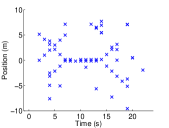
(a)

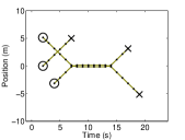
(b)

Figure 6: Scenario of the simulation: (a) Observed sequence of measurements. At time 14, there are two measurements close together at positions 5.45 and 5.47. (b) Trajectories from which the measurements have been generated. Circles and crosses indicate the start and end of trajectories.

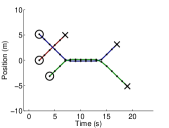
(a) 0.42

(b) 0.12

(c) 0.12

(d) 0.04

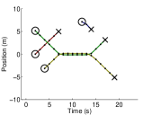
(e) 0.02

(f) 0.02

Figure 7: Posterior mean of the trajectories for the six global hypotheses with largest weights, which are given in the subfigure captions. Colors for different trajectories are only used to help visualisation, they are not labels.

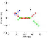
(a)

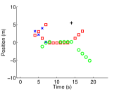
(b)

Figure 8: Two equally likely estimates provided by the $\delta$-GLMB filter. Different markers represent different labels. Track formation using multitarget filtering densities does not work well due to track switching that can happen for targets born at the same time.

We now consider another scenario with the same parameters but with $\kappa\left(z\right)=\frac{1}{20}1_{\left(-10,10\right)}\left(z\right)$ and $R=10^{-3}$, i.e., lower clutter and higher measurement noise. We show the observed measurements and the three most likely hypotheses in Figure 9. None of the three most likely global hypotheses has two trajectories that start at time 2 as the trajectories that were used to generate the measurements, see Figure 6(b). This is due to the fact that one of the trajectories has not been detected at time 2, see Figure 9(a). The third most likely global hypothesis includes a trajectory switching when targets are in close proximity.

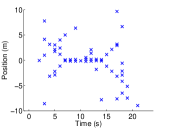
(a)

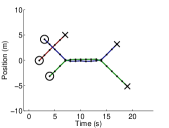
(b) 0.21

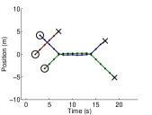
(c) 0.14

(d) 0.08

Figure 9: Measurements and three most likely global hypotheses. Their weights are given in the subfigure captions. The third most likely global hypothesis includes a trajectory switching.

V-B Two dimensional scenario

We consider that a target state $x\in\mathbb{R}^{4}$ that includes the position and velocity in a two dimensional space. The birth process has parameters: $b=2$, $\beta_{1}\left(x\right)=\beta_{2}\left(x\right)=\mathcal{N}\left(x;\left[500,2,500,2\right]^{T},\mathrm{diag}\left(250^{2},5^{2},250^{2},5^{2}\right)\right)$, $w_{B}\left(\oslash\right)=0.85$, $w_{B}\left(\left\{1\right\}\right)=w_{B}\left(\left\{2\right\}\right)=0.05$, $w_{B}\left(\left\{1,2\right\}\right)=0.05$, where it should be noted that the two targets can be born in a large area, not at a very specific location. The single-target dynamic process parameters are: $p_{S}=0.99$, $g\left(x^{i}|x^{i-1}\right)=\mathcal{N}\left(x^{i};Fx^{i-1},Q\right)$ with

$$F=I_{2}\otimes \left(\begin{array}[]{cc}1&\tau\\ 0&1\end{array}\right),\quad Q=qI_{2}\otimes\left(\begin{array}[]{cc}\tau^{3}/3&\tau^{2}/2\\ \tau^{2}/2&\tau\end{array}\right),$$

where $\otimes$ denotes Kronecker product, $\tau$ is the sampling time and $q$ is a parameter of the model. We use $\tau=1$, $q=0.25$ and we consider a total number of $k_{f}=150$ steps in the simulations.

The intensity function of the Poisson clutter is $\kappa\left(z\right)=70\cdot\frac{1}{10^{6}}1_{A}\left(z\right)$, which means that clutter is uniformly distributed in an area $\left(0,1000\right)\times\left(0,1000\right)$ and there is an average of $70$ clutter measurement per scan. The position of each target is measured with parameters: $p_{D}=0.9$ and $l\left(z|x\right)=\mathcal{N}\left(z;Hx,R\right)$ where $R=I_{2}$ and

$$H= \left(\begin{array}[]{cccc}1&0&0&0\\ 0&0&1&0\end{array}\right).$$

The prediction and update steps of the trajectory $\mathrm{MBM}_{01}$ filter are computed as indicated in Appendix E. The maximum number of global hypotheses we consider is $N_{h}=300$. At each update step, we use ellipsoidal gating [10] with threshold 10 to consider only the relevant measurements for each single trajectory hypothesis. In addition, for each global hypothesis, we use Murty’s algorithm to select the $k_{m}$-best new global hypotheses without having to evaluate the weights of all the new global hypotheses. The cost matrix of Murty’s algorithm is the same as in the $\delta$-GLMB filter, as the new data associations only depend on the target states at the current time. As in [18], for a global hypothesis with a weight $w^{k|k-1}\left(\cdot\right)$, we set $k_{m}$ to $\left\lceil N_{h}\cdot w^{k|k-1}\left(\cdot\right)\right\rceil$. Once the new global hypotheses are formed, pruning is performed to keep the $N_{h}$ global hypotheses with highest weights. For the prediction step, we use the $k_{p}$-shortest path algorithm to prune the number of predicted hypotheses of the surviving trajectories, as in [17]. We select $k_{p}$ as $\left\lceil 3\cdot N_{h}\cdot w^{k|k}\left(\cdot\right)\right\rceil$.

Also, each trajectory density is propagated using an $L$-scan sliding window. That is, as explained in [29], an $L$-scan trajectory density considers a joint density over the last $L$ time steps of the trajectory and the rest of the time steps are considered independent. Therefore, for past states beyond the $L$-scan window, we only need to store the means and covariance matrices for the corresponding target state at each each time step. Moreover, if one is only interested in estimation, and not in the underlying uncertainty, one can simply store the trajectory means outside the $L$-scan window for each trajectory density. At each time step, we can estimate the true sets of trajectories, for example, by considering the posterior means of the trajectories for the global hypothesis with highest weight.

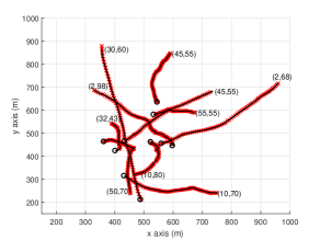
Figure 10: The ten true trajectories are shown as black lines. The initial position of a true trajectory is marked with a black circle and its $\left(t,i\right)$, starting time and duration, is indicated next to its end position. The posterior means of the trajectories for the global hypothesis with highest weight of the trajectory $\mathrm{MBM}_{01}$ filter at the final time step are shown with red lines and crosses.

We consider 10 true trajectories, which have been obtained by sampling from the dynamic model, and are shown in Figure 10. We first consider one realisation of the measurements so that we can also plot the posterior means of the trajectories for the global hypothesis with highest weight at the end of the simulation. In Figure 10, the single trajectory densities have been propagated using $L=2$. We can see that the conjugate prior can be used to successfully estimate the true set of trajectories. No false trajectories are reported, though some trajectories are detected after some delay. It should be noted that changing $L$ does not affect the weights of the hypotheses or the available information on the targets at the current time step. Increasing $L$ only improves the knowledge we have about past states of a trajectory. Also, if we set $L=1$, we have an algorithm that does not perform trajectory smoothing. That is, for $L=1$, we run a Kalman filter to obtain the mean and covariance matrix at the current time, for each single trajectory hypothesis, and all the previously obtained means (and optionally the covariance matrices) are stored. In fact, for $L=1$ and the pruning of the predicted and updated hypotheses explained above, the trajectory $\mathrm{MBM}_{01}$ filter and the $\delta$-GLMB filter perform the same computational operations. However, the trajectory $\mathrm{MBM}_{01}$ filter with $L=1$ requires more storage than $\delta$-GLMB to keep information about past states of the trajectories for all single trajectory hypotheses, including dead ones. Also, estimation is performed in a different manner in which a trajectory estimate is obtained from the same single trajectory hypothesis at all time steps. This avoids track switching of the type shown in Figure 3(b).

The running times to process the 150 time steps using a non-optimised Matlab implementation on an Intel Xeon CPU at 3.5 GHz for different values of $L$ are: 143.2 s (1-scan/$\delta$-GLMB filter), 144.4 s (2-scan), 145.7 s (5-scan) and 159.7 s (10-scan). It is important to notice that the computational burden for $L$ between 1 and 5 is quite similar. This implies that, for values of $L$ between 1 and 5, most of the computational burden is related to how hypotheses are handled, and improving the knowledge we have about past trajectory states requires a small computational cost.

We would like to mention that, with the considered pruning parameters, the global hypothesis with highest weight does not consider two targets born at the same time, despite the fact that this is the ground truth situation. If we increase the number of global hypotheses to 4000, the global hypothesis with highest weight includes two targets born at time step 2. In this case, the $\delta$-GLMB filter shows track switching for the two targets born at time step 2, as was illustrated in Figure 8. This illustration is omitted in this example as it has been illustrated before. This track switching can also be avoided by considering sequences of sets of labelled targets. However, the only algorithm available in the literature [25] is a batch algorithm, so it is not addressing the same problem, and is based on sampling of trajectories and data associations, which is not necessary for linear/Gaussian problems.

We proceed to analyse the error in the final trajectory estimates obtained by the trajectory $\mathrm{MBM}_{01}$ filter and the $\delta$-GLMB filter using Monte Carlo simulation with $N_{mc}=100$ runs. In order to do so, we calculate the root mean square optimal assignment sub-pattern assignment (OSPA) [44, 13] error and the root mean square GOSPA [45] for the position elements across all time steps. Both metrics use the Euclidean metric as the base metric, $p=2$ and $c=15$. The GOSPA metric $d\left(\cdot,\cdot\right)$ uses $\alpha=2$ as this choice enables the decomposition of the error into localisation error for properly detected targets and costs for missed and false targets [45] such that

$$d^{2}\left(\mathbf{x}^{k},\mathbf{\hat{x}}_{i}^{k}\right) =c_{l}^{2}\left(\mathbf{x}^{k},\mathbf{\hat{x}}_{i}^{k}\right)+c_{m}^{2}\left(\mathbf{x}^{k},\mathbf{\hat{x}}_{i}^{k}\right)+c_{f}^{2}\left(\mathbf{x}^{k},\mathbf{\hat{x}}_{i}^{k}\right)$$

where $c_{l}^{2}\left(\cdot,\cdot\right)$, $c_{m}^{2}\left(\cdot,\cdot\right)$, and $c_{f}^{2}\left(\cdot,\cdot\right)$ are the squared cost for localisation error, missed targets and false targets, respectively.

The root mean square GOSPA/OSPA error across all time steps is

$$\mathrm{RMSGOSPA} =\sqrt{\frac{1}{N_{mc}k_{f}}\sum_{i=1}^{N_{mc}}\sum_{k=1}^{k_{f}}d^{2}\left(\mathbf{x}^{k},\mathbf{\hat{x}}_{i}^{k}\right)}$$ (30)

where $\mathbf{x}^{k}$ is the set of targets at time $k$ and $\mathbf{\hat{x}}_{i}^{k}$ is the estimated set of targets at time $k$ in the $i$-th Monte Carlo runs. The resulting errors as well as the root mean square errors for the decomposition of the GOSPA metric are shown in Table I. Increasing the value of $L$ lowers GOSPA/OSPA errors. From the GOSPA decomposition, we can see that increasing $L$ lowers the localisation error for properly detected targets, but does not change the cost for missed and false targets. The cost for missed and false targets does not change, as in this case, $L=1$ is sufficient to estimate the target states within a radius of $c$. In addition, the main source of GOSPA error for any $L$ are missed target costs and localisation errors. False target costs are smaller. For any value of $L$, the proposed algorithm based on sets of trajectories outperforms the $\delta$-GLMB filter for both GOSPA and OSPA metrics.

In Table I, we also show the root mean square error for the position elements using the metric for sets of trajectories in [26] based on linear programming (LP), with parameters $p=2$ and $c=15$ and $\gamma=1$. This metric, apart from penalising localisation errors for properly detected targets, missed and false targets, it also penalises track switches, and it can be decomposed into its different components in a manner similar to GOSPA. As expected, the $\delta$-GLMB filter has a higher error related to track switches than the trajectory $\mathrm{MBM}_{01}$ filter.

Table I: Root mean square OSPA/GOSPA/LP metric errors

Algorithm	Trajectory $\mathrm{MBM}_{01}$			$\delta$-GLMB
$L$	1	2	5	-
OSPA	38.54	37.28	36.93	64.83
GOSPA	58.34	53.37	51.99	90.56
GOSPA-Localisation	33.22	23.40	20.06	31.52
GOSPA-Missed	44.18	44.18	44.18	74.73
GOSPA-False	18.67	18.67	18.67	40.29
LP trajectory metric	58.35	53.37	51.99	91.12
LP-Localisation	33.21	23.40	20.06	31.52
LP-Missed	44.18	44.18	44.18	74.73
LP-False	18.67	18.67	18.67	40.51
LP-Switches	0.66	0.63	0.63	2.32

VI Conclusions

In this paper, we have proposed the set of trajectories as the variable of interest in MTT and have indicated how to use Mahler’s RFS framework on this variable to fully characterise the MTT problem with targets without a priori identification. Using the multitrajectory density on sets of trajectories, we can answer all trajectory related questions. Set of trajectories also enable us to define metrics with physical interpretation, which can be used to obtain optimal estimators and evaluate algorithms. Therefore, sets of trajectories along with Mahler’s RFS framework enable us to perform all the tasks of MTT.

We have also derived a conjugate multitrajectory density that gives rise to the trajectory $\mathrm{MBM}_{01}$ filter to compute multitrajectory filtering density. In addition, we have described relations with other labelled and unlabelled RFS models and MHT. Finally, we have illustrated via simulations how we can perform MTT using sets of trajectories.

Future work includes the specification of the measure theory aspects for sets of trajectories, the development of computationally efficient algorithms for MTT based on sets of trajectories and the inclusion of target spawning.

Appendix A

FISST can be applied with a single object space that is locally compact, Hausdorff and second-countable (LCHS) [12, Sec. 2.2.2]. In Appendix A-A, we prove that the trajectory space $T_{\left(k^{\prime}\right)}$ up to time step $k^{\prime}$ is LCHS so we can use FISST with sets of trajectories. In Appendix A-B, we explain how the single trajectory integral and the set integral are defined.

A-A The space $T_{\left(k^{\prime}\right)}$ is LCHS

The trajectory space $T_{\left(k^{\prime}\right)}$ up to a certain time step $k^{\prime}$ is the disjoint union, which is also called the direct sum [46], of a finite number of subspaces, for which one can define the disjoint union topology [47]. As $D^{i}$ is a Euclidean space, $D^{i}$ is locally compact and Hausdorff. Then, it is direct to show that $\left\{t\right\}\times D^{i}$ is locally compact and Hausdorff. The disjoint union of Hausdorff spaces is Hausdorff [48], so $T_{\left(k^{\prime}\right)}$ is Hausdorff. The disjoint union of locally compact spaces is locally compact [46], so $T_{\left(k^{\prime}\right)}$ is locally compact.

In order to prove that $T_{\left(k^{\prime}\right)}$ is second-countable, which is synonymous to completely separable and implies separability [49], we first recall two definitions. A space $E$ is second-countable if and only if its topology has a countable base [47, page 108]. A base in a space $E$ is a collection of open sets in $E$ such that every open set in $E$ can be written as a union of elements of the base [47, page 38]. The space $D^{i}=\mathbb{R}^{in_{x}}$, with the usual topology, is second-countable with a countable base $\mathcal{B}_{1}\left(i\right)$, which denotes the collection of open balls centred on all rational points in $D^{i}$ with all rational radius [49, page 100].

We proceed to prove that $T_{\left(k^{\prime}\right)}$ is second-countable with countable base $\mathcal{B}_{2}=\uplus_{t\text{=1}}^{k^{\prime}}\left\{t\right\}\times\uplus_{i=1}^{k^{\prime}-t+1}\mathcal{B}_{1}\left(i\right)$. It is direct to see that the space $\left\{t\right\}\times\mathbb{R}^{in_{x}}$ is second-countable with a countable base $\left\{t\right\}\times\mathcal{B}_{1}\left(i\right)$. In addition, due to the disjoint union topology, a set in $S\subseteq T_{\left(k^{\prime}\right)}$ is open if and only if $S\cap\left(\left\{t\right\}\times D^{i}\right)$ is open for all $\left(t,i\right)\in I_{(k^{\prime})}$. Also, since $S$ is the union of the sets $S\cap\left(\left\{t\right\}\times D^{i}\right)$ for all $\left(t,i\right)\in I_{(k^{\prime})}$, it follows that any open set $S$ can be written as a union of elements of $\mathcal{B}_{2}$, which is a countable set. This proves that the single trajectory space is second-countable.

A-B Integrals

In FISST, if the single object space is the disjoint union of subspaces, each endowed with an integral, the single object integral is the sum of the integrals over each subspace [12, Sec. 3.5.3]. In the trajectory case, $T_{\left(k^{\prime}\right)}=\uplus_{\left(t,i\right)\in I_{(k^{\prime})}}\left\{t\right\}\times D^{i}$ where $\left\{t\right\}\times D^{i}$ is the Cartesian product of a single element set and a Euclidean space, for which the discrete-Lebesgue integral exists. Therefore, the single trajectory integral is given by (3). Following [12, Sec. 3.5.3], the corresponding set integral on $\mathcal{F}\left(T_{\left(k^{\prime}\right)}\right)$ is given by (4). Single object spaces that are the disjoint union of spaces of different dimensionality, as the single trajectory space, have been used for RFSs in [12, Sec. 2.2.2, Sec. 11.6, Chap. 18][50].

Based on set integrals and multi-object densities, one can define probability generating functionals [28, Eq. (44)], which can be used to derive filters. It is also possible to define measure theoretic integrals for functions on sets in LCHS spaces [37, App. B], which can be used to define probability densities, though it is beyond the scope of this paper to present the details.

Appendix B

We explain the connection between multitarget densities and Janossy densities [51] and how to calculate probabilities.

B-A Target case

A multitarget density packages the entire family of Janossy densities into a single function [28, p. 1161]. Given a multiobject density $\pi\left(\cdot\right)$, we can obtain the equivalent $n$th Janossy density $j_{n}\left(\cdot\right)$ as [28, Sec. II.D],

$$j_{n}\left(x_{1},...,x_{n}\right) =\pi\left(\left\{x_{1},...,x_{n}\right\}\right).$$ (31)

The Janossy density $j_{n}\left(\cdot\right)$ is the density of the $n$th Janossy measure w.r.t. the Lebesgue measure on $D^{n}$ [51, p. 124]. Then,

$$j_{n}\left(x_{1},...,x_{n}\right)dx_{1}...dx_{n}$$ (32)

is the probability that there are exactly $n$ points in the process, one in each of the $n$ distinct infinitesimal regions $\left(x_{i},x_{i}+dx_{i}\right)\subset D$ [51].

We define a region $A=\uplus_{n\text{=0}}^{\infty}A_{n}$ where $A_{n}\subseteq\mathcal{F}\left(D\right)$ is a set that contains sets with $n$ elements in $D$. Then, for $\mathbf{x}$ distributed as $\pi\left(\cdot\right)$,

$$P\left(\mathbf{x}\in A\right) =\sum_{n=0}^{\infty}P\left(\left\{x_{1},...,x_{n}\right\}\in A_{n}\right)$$

$$=\sum_{n=0}^{\infty}P\left(x_{1:n}\in\chi^{-1}\left(A_{n}\right)\right)$$

$$=\sum_{n=0}^{\infty}\frac{1}{n!}\int_{\chi^{-1}\left(A_{n}\right)}j_{n}\left(x_{1:n}\right)dx_{1:n}$$

$$=\sum_{n=0}^{\infty}\frac{1}{n!}\int_{\chi^{-1}\left(A_{n}\right)}\pi\left(\left\{x_{1},...,x_{n}\right\}\right)dx_{1:n}.$$ (33)

where $\chi\left(\cdot\right)$ denotes the mapping from vectors to sets, as indicated in Section II-C for trajectories or in [37].

B-B Trajectory case

By analogy to (31)-(32), for a multitrajectory density $\pi\left(\cdot\right)$,

$$\pi\left(\left\{\left(t_{1},x_{1}^{1:i_{1}}\right),...,\left(t_{n},x_{n}^{1:i_{n}}\right)\right\}\right)dx_{1}^{1:i_{1}}...dx_{n}^{1:i_{n}}$$

is the probability that there are exactly $n$ distinct trajectories, with starting times and lengths $t_{1},i_{1},...,t_{n},i_{n}$ in infinitesimal regions $\left(x_{j}^{1:i_{j}},x_{j}^{1:i_{j}}+dx_{j}^{1:i_{j}}\right)\subset D^{i_{j}}$. For $\mathbf{X}$ distributed according to $\pi\left(\cdot\right)$ and a region $A=\uplus_{n\text{=0}}^{\infty}A_{n}$, where $A_{n}\subseteq\mathcal{F}\left(T_{\left(k^{\prime}\right)}\right)$ is a set that contains sets with $n$ elements in $T_{\left(k^{\prime}\right)}$, we have

$$P\left(\mathbf{X}\in A\right) =\sum_{n=0}^{\infty}P\left(\left\{X_{1},...,X_{n}\right\}\in A_{n}\right)$$

$$=\sum_{n=0}^{\infty}\frac{1}{n!}\int_{\chi^{-1}\left(A_{n}\right)}\pi\left(\left\{X_{1},...,X_{n}\right\}\right)dX_{1:n}.$$

Appendix C

In this appendix, we prove Theorem 7. First, we provide the transition density. Given $X=\left(t,x^{1:i}\right)$ with $t+i-1<k$ and $Y=\left(t^{\prime},y^{1:i^{\prime}}\right)$, the single trajectory transition density at time $k$ is

$$g^{k}\left(Y\left|X\right.\right) =\left|\tau^{k-1}\left(X\right)\right|\left[\vphantom{\delta\left(\left(t^{\prime},y^{1:i^{\prime}-1}\right)-X\right)}\left(1-p_{S}\left(x^{i}\right)\right)\delta_{X}\left(Y\right)\right.$$

$$\quad\left.+p_{S}\left(x^{i}\right)g\left(y^{i^{\prime}}|x^{i}\right)\delta_{X}\left(\left(t^{\prime},y^{1:i^{\prime}-1}\right)\right)\right]$$

$$\quad+\left(1-\left|\tau^{k-1}\left(X\right)\right|\right)\delta_{X}\left(Y\right).$$ (34)

That is, if the trajectory has died before time step $k-1$, the trajectory remains unaltered with probability one. If the trajectory exists at time step $k-1$, it remains unaltered (target dies) with probability $\left(1-p_{S}\left(\cdot\right)\right)$ or the last target state is generated according to the single target transition density with probability $p_{S}\left(\cdot\right)$. Without target births, the number of trajectories remains unchanged so the transition density for the sets of trajectories is [8, Eq. (12.91)]

$$g^{k}\left(\left\{Y_{1},...,Y_{n}\right\}\left|\left\{X_{1},...,X_{n}\right\}\right.\right) =\sum_{\sigma\in\Gamma_{n}}\prod_{j=1}^{n}g^{k}\left(Y_{\sigma_{j}}\left|X_{j}\right.\right)$$ (35)

where $\Gamma_{n}$ is the set that includes all the permutations of $\left(1,...,n\right)$.

We evaluate $\pi^{k|k-1}\left(\cdot\right)$ for $\mathbf{W}\uplus\mathbf{X}\uplus\mathbf{Y}\uplus\mathbf{Z}$, where these sets are defined in Theorem 7. The multitrajectory density for set $\mathbf{X}\uplus\mathbf{Y}\uplus\mathbf{Z}$ (no births) is denoted by $\pi_{S}^{k|k-1}\left(\cdot\right)$ and the multitrajectory density for set $\mathbf{W}$ by $\beta^{k}\left(\cdot\right)$. Using the convolution formula [12, Sec. 4.2.3], we have

$$\pi^{k|k-1}\left(\mathbf{W}\uplus\mathbf{X}\uplus\mathbf{Y}\uplus\mathbf{Z}\right)$$

$$=\sum_{\mathbf{A}\subseteq\mathbf{W}\uplus\mathbf{X}\uplus\mathbf{Y}\uplus\mathbf{Z}}\pi_{S}^{k|k-1}\left(\mathbf{W}\uplus\mathbf{X}\uplus\mathbf{Y}\uplus\mathbf{Z}\setminus\mathbf{A}\right)\beta^{k}\left(\mathbf{A}\right).$$

As $\beta^{k}\left(\cdot\right)$ is zero unless evaluated at a set of new born trajectories, $\beta^{k}\left(\mathbf{A}\right)$ is different from zero only if $\mathbf{A}=\mathbf{W}$, which yields

$$\pi^{k|k-1}\left(\mathbf{W}\uplus\mathbf{X}\uplus\mathbf{Y}\uplus\mathbf{Z}\right) =\pi_{S}^{k|k-1}\left(\mathbf{X}\uplus\mathbf{Y}\uplus\mathbf{Z}\right)\beta^{k}\left(\mathbf{W}\right)$$

where

$$\beta^{k}\left(\mathbf{W}\right) =\beta_{\tau}\left(\tau^{k}\left(\mathbf{W}\right)\right)$$

as the states of new born trajectories are distributed according to the multiobject density $\beta_{\tau}\left(\cdot\right)$ and the birth time and length are deterministic.

On the other hand, the multitrajectory density for the surviving targets is given by the prediction step, with the transition density without target births which is given in (35). Then,

$$\pi_{S}^{k|k-1}\left(\mathbf{X}\uplus\mathbf{Y}\uplus\mathbf{Z}\right) =\int g^{k}\left(\mathbf{X}\uplus\mathbf{Y}\uplus\mathbf{Z}\left|\mathbf{W}^{\prime}\right.\right)\pi^{k-1}\left(\mathbf{W}^{\prime}\right)\delta\mathbf{W}^{\prime},$$

Partitioning $\mathbf{W}^{\prime}=\mathbf{D}\uplus\mathbf{A}$, where $\mathbf{D}$ and $\mathbf{A}$ represent dead and alive trajectories at time $k-1$, the set integral over $\mathbf{W}^{\prime}$ can be calculated as the set integral over $\mathbf{D}$ and $\mathbf{A}$ [12, Sec. 3.5.3]

$$\pi_{S}^{k|k-1}\left(\mathbf{X}\uplus\mathbf{Y}\uplus\mathbf{Z}\right)$$

$$\quad=\int\int g^{k}\left(\mathbf{X}\uplus\mathbf{Y}\uplus\mathbf{Z}\left|\mathbf{D}\uplus\mathbf{A}\right.\right)\pi^{k-1}\left(\mathbf{D}\uplus\mathbf{A}\right)\delta\mathbf{D}\delta\mathbf{A}$$

$$\quad=\int g^{k}\left(\mathbf{X}\uplus\mathbf{Y}\left|\mathbf{A}\right.\right)\pi^{k-1}\left(\mathbf{Z}\uplus\mathbf{A}\right)\delta\mathbf{A}.$$

Evaluating this expression for $\mathbf{X}=\left\{X_{1},...,X_{m}\right\}$ and $\mathbf{Y}=\left\{Y_{1},...,Y_{n}\right\}$ and using (35), we have

$$\pi_{S}^{k|k-1}\left(\mathbf{X}\uplus\mathbf{Y}\uplus\mathbf{Z}\right)$$

$$=\frac{1}{\left(m+n\right)!}\int\sum_{\sigma\in\Gamma_{m+n}}\prod_{j=1}^{{}_{m}}g^{k}\left(X_{j}|A_{\sigma\left(j\right)}\right)$$

$$\times\prod_{j=m+1}^{{}_{m+n}}g^{k}\left(Y_{j-m}|A_{\sigma\left(j\right)}\right)$$

$$\times\pi^{k-1}\left(\mathbf{Z}\uplus\left\{A_{1},...,A_{m+n}\right\}\right)dA_{1:m+n}$$

$$=\int\prod_{j=1}^{{}_{m}}g^{k}\left(X_{j}|A_{j}\right)\prod_{j=m+1}^{{}_{m+n}}g^{k}\left(Y_{j-m}|A_{j}\right)$$

$$\quad\quad\times\pi^{k-1}\left(\mathbf{Z}\uplus\left\{A_{1},...,A_{m+n}\right\}\right)dA_{1:m+n}.$$ (36)

The proof is finished by substituting (34) into (36).

Appendix D

In this appendix, we prove that the birth model (16) is an $\mathrm{MBM}_{01}$. We also prove Lemmas 9 and 10.

D-A Birth model

We write (16) as

$$\beta_{\tau}\left(\left\{x_{1},...,x_{n}\right\}\right)$$

$$\quad=\sum_{l_{1:n}}^{\neq}\left(\sum_{L\subseteq\mathbb{N}_{b}}w_{B}\left(L\right)\delta_{L}\left(\left\{l_{1},...,l_{n}\right\}\right)\right)\prod_{j=1}^{n}\beta_{l_{j}}\left(x_{j}\right)$$

$$\quad=\sum_{L\subseteq\mathbb{N}_{b}}w_{B}\left(L\right)\left(\sum_{l_{1:n}}^{\neq}\delta_{L}\left(\left\{l_{1},...,l_{n}\right\}\right)\prod_{j=1}^{n}\beta_{l_{j}}\left(x_{j}\right)\right)$$

where $\delta_{L}\left(\cdot\right)$ is the Kronecker delta for sets: $\delta_{L}\left(\left\{l_{1},...,l_{n}\right\}\right)=1$ if $\left\{l_{1},...,l_{n}\right\}=L$ and zero otherwise. From [8, Eq. (11.133)], we can see that the factor inside the bracket is a multi-Bernoulli density such that the probabilities of existence of the Bernoulli components whose indices belong to $L$ are one and the rest are zero. The corresponding single-target density for $l_{j}\in\mathbb{N}_{b}$ is $\beta_{l_{j}}\left(\cdot\right)$. Therefore, the birth model is a mixture of multi-Bernoulli densities whose existence probabilities are either 0 or 1 and the weight of each mixture component is given by $w_{B}\left(L\right)$ $L\subseteq\mathbb{N}_{b}$. Analogously, one can check that the multitrajectory filtering and predicted densities, which are given by (17) and (18), are also $\mathrm{MBM}_{01}$.

D-B Prediction

We consider the sets $\mathbf{W}=\left\{W_{1},...,W_{n_{w}}\right\}$, $\mathbf{X}=\left\{X_{1},...,X_{n_{x}}\right\}$, $\mathbf{Y}=\left\{Y_{1},...,Y_{n_{y}}\right\}$ and $\mathbf{Z}=\left\{Z_{1},...,Z_{n_{z}}\right\}$, as defined in Theorem 7. We also denote $n_{xyz}=n_{x}+n_{y}+n_{z}$, $n_{xyzw}=n_{x}+n_{y}+n_{z}+n_{w}$ and $X_{j}=\left(t_{j},x_{j}^{1:i_{j}}\right)$. Substituting (16) and (17) into Theorem 7 yields

$$\pi^{k|k-1}\left(\mathbf{W}\uplus\mathbf{X}\uplus\mathbf{Y}\uplus\mathbf{Z}\right)$$

$$=\sum_{h_{1:n_{xyz}}^{k-1|k-1}}^{\neq}w^{k-1|k-1}\left(\left\{h_{1}^{k-1|k-1},...,h_{n_{xyz}}^{k-1|k-1}\right\}\right)$$

$$\times\prod_{j=1}^{n_{x}}\left[g\left(x_{j}^{i_{j}}\left|x_{j}^{i_{j}-1}\right.\right)p_{S}\left(x_{j}^{i_{j}-1}\right)\right.$$

$$\,\left.\times p^{k-1|k-1}\left(t_{j},x_{j}^{1:i_{j}-1}|h_{j}^{k-1|k-1}\right)\right]$$

$$\,\times\prod_{j=1}^{n_{y}}\left[\left(1-p_{S}\left(Y_{j}^{|}\right)\right)p^{k-1|k-1}\left(Y_{j}|h_{j+n_{x}}^{k-1|k-1}\right)\right]$$

$$\,\times\prod_{j=1}^{n_{z}}p^{k-1|k-1}\left(Z_{j}|h_{j+n_{x}+n_{y}}^{k-1|k-1}\right)$$

$$\,\times\sum_{h_{n_{xyz}+1:n_{xyzw}}^{k|k-1}}^{\neq}w_{B}^{k}\left(\left\{h_{n_{xyz}+1}^{k|k-1},...,h_{n_{xyzw}}^{k|k-1}\right\}\right)$$

$$\,\times\prod_{j=1}^{n_{w}}p_{N}^{k|k-1}\left(W_{j}|h_{j+n_{xyz}}^{k|k-1}\right)$$

where we should note that $w_{B}^{k}\left(\cdot\right)$ is zero for hypotheses that are not contained in $\mathbb{N}^{k}$.

We can also express the above summations in terms of the hypotheses $h_{j}^{k|k-1}$ instead of $h_{j}^{k-1|k-1}$. The relation between the hypotheses is

$$h_{j}^{k-1|k-1} =\begin{cases}\left(h_{j}^{k|k-1}\right)^{-}&j=1,...,n_{x}\\ h_{j}^{k|k-1}&j=n_{x}+1,...,n_{xyz}\end{cases}$$

where $\left(h_{j}^{k|k-1}\right)^{-}$ is defined in Lemma 9. We can then write

$$\pi^{k|k-1}\left(\mathbf{W}\uplus\mathbf{X}\uplus\mathbf{Y}\uplus\mathbf{Z}\right)$$

$$=\sum_{h_{1:n_{xyzw}}^{k|k-1}}^{\neq}w^{k-1|k-1}\left(\left\{\left(h_{1}^{k|k-1}\right)^{-},...,\left(h_{n_{x}}^{k|k-1}\right)^{-}\right\}\right.$$

$$\quad\left.\vphantom{\left(h_{1}^{k|k-1}\right)^{-}}\cup\left\{h_{n_{x}+1}^{k|k-1},...,h_{n_{x}+n_{y}}^{k|k-1}\right\}\cup\left\{h_{n_{x}+n_{y}+1}^{k|k-1},...,h_{n_{xyz}}^{k|k-1}\right\}\right)$$

$$\,\times w_{B}^{k}\left(\left\{h_{n_{xyz}+1}^{k|k-1},...,h_{n_{xyzw}}^{k|k-1}\right\}\right)$$

$$\,\times\prod_{j=1}^{n_{x}}\gamma_{S}\left(h_{j}^{k|k-1}\right)\prod_{j=1}^{n_{y}}\gamma_{D}\left(h_{j+n_{x}}^{k|k-1}\right)\prod_{j=1}^{n_{x}}p_{S}^{k|k-1}\left(X_{j}|h_{j}^{k|k-1}\right)$$

$$\,\times\prod_{j=1}^{n_{y}}p_{D}^{k|k-1}\left(Y_{j}|h_{j+n_{x}}^{k|k-1}\right)\prod_{j=1}^{n_{z}}p^{k-1|k-1}\left(Z_{j}|h_{j+n_{x}+n_{y}}^{k|k-1}\right)$$

$$\,\times\prod_{j=1}^{n_{w}}p_{N}^{k|k-1}\left(W_{j}|h_{j+n_{xyz}}^{k|k-1}\right).$$

Note that, as $\mathbf{X}$, $\mathbf{Y}$, $\mathbf{Z}$ and $\mathbf{W}$ represent surviving, dying, dead and new born trajectories, one must have that sets of hypotheses $\mathcal{A}=\left\{h_{1}^{k|k-1},...,h_{n_{x}}^{k|k-1}\right\}$, $\mathcal{B}=\left\{h_{n_{x}+1}^{k|k-1},...,h_{n_{x}+n_{y}}^{k|k-1}\right\}$, $\mathcal{D}=\left\{h_{n_{x}+n_{y}+1}^{k|k-1},...,h_{n_{xyz}}^{k|k-1}\right\}$ and $\mathcal{C}=\left\{h_{n_{xyz}+1}^{k|k-1},...,h_{n_{xyzw}}^{k|k-1}\right\}$ represent surviving, dying, dead and new born trajectory hypotheses. Otherwise, the corresponding terms in the sum over all hypotheses are equal to zero. Therefore, given $\mathcal{A}$, $\mathcal{B}$, $\mathcal{D}$ and $\mathcal{C}$, we can identify the weight $w^{k|k-1}\left(\cdot\right)$ of the predicted global hypothesis $\mathcal{A}\uplus\mathcal{B}\uplus\mathcal{C}\uplus\mathcal{D}$, as the factors in front of the densities in the previous expression. The resulting weight and single trajectory densities can be written as in Lemma 9, which concludes its proof.

D-C Update

The predicted density (18) evaluated at a set $\mathbf{X}=\left\{X_{1},...,X_{n_{x}}\right\}$ of alive trajectories and a set $\mathbf{Y}=\left\{Y_{1},...,Y_{n_{y}}\right\}$ of dead trajectories can be written as

$$\pi^{k|k-1}\left(\mathbf{X}\uplus\mathbf{Y}\right)$$

$$=\sum_{h_{1:n_{x}+n_{y}}^{k|k-1}}^{\neq}\prod_{j=1}^{n_{x}}p^{k|k-1}\left(X_{j}|h_{j}^{k|k-1}\right)\prod_{j=1}^{n_{y}}p^{k|k-1}\left(Y_{j}|h_{j+n_{x}}^{k|k-1}\right)$$

$$\,\times w^{k|k-1}\left(\left\{h_{1}^{k|k-1},...,h_{n_{{}_{x}}}^{k|k-1}\right\}\cup\left\{h_{n_{x}+1}^{k|k-1},...,h_{n_{x}+n_{{}_{y}}}^{k|k-1}\right\}\right)$$

$$=\sum_{h_{1:n_{x}}^{k|k-1}}^{\neq}\sum_{h_{n_{x}+1:n_{x}+n_{y}}^{k|k-1}}^{\neq}\prod_{j=1}^{n_{x}}p^{k|k-1}\left(X_{j}|h_{j}^{k|k-1}\right)$$

$$\,\times\prod_{j=1}^{n_{y}}p^{k|k-1}\left(Y_{j}|h_{j+n_{x}}^{k|k-1}\right)$$

$$\,\times w^{k|k-1}\left(\left\{h_{1}^{k|k-1},...,h_{n_{{}_{x}}}^{k|k-1}\right\}\cup\left\{h_{n_{x}+1}^{k|k-1},...,h_{n_{x}+n_{{}_{y}}}^{k|k-1}\right\}\right).$$

As $\mathbf{X}$ and $\mathbf{Y}$ are sets of alive and dead trajectories, the terms in the above summation are zero unless $h_{1:n_{x}}^{k|k-1}\in\left(\mathbb{U}^{k}\right)^{n_{x}}$ and $h_{n_{x}+1:n_{x}+n_{y}}^{k|k-1}\in\left(\mathbb{D}^{1:k}\right)^{n_{y}}$, which represent alive and dead single trajectory hypotheses, respectively.

Substituting the previous equation and (12) into (11), the updated density is

$$\pi^{k}\left(\mathbf{X}\uplus\mathbf{Y}\right)$$

$$\propto\sum_{\theta\in\Theta_{n_{x},m}}\sum_{h_{1:n_{x}}^{k|k-1}}^{\neq}\sum_{h_{n_{x}+1:n_{x}+n_{y}}^{k|k-1}}^{\neq}\prod_{j=1}^{n_{y}}p^{k|k-1}\left(Y_{j}|h_{j+n_{x}}^{k|k-1}\right)$$

$$\quad\times\prod_{j=1}^{n_{x}}\left[\psi_{\mathbf{z}^{k}}\left(X_{j}|\theta_{j}\right)p^{k|k-1}\left(X_{j}|h_{j}^{k|k-1}\right)\right]$$

$$\,\times w^{k|k-1}\left(\left\{h_{1}^{k|k-1},...,h_{n_{{}_{x}}}^{k|k-1}\right\}\cup\left\{h_{n_{x}+1}^{k|k-1},...,h_{n_{x}+n_{{}_{y}}}^{k|k-1}\right\}\right)$$

$$=\sum_{\left(h_{1}^{k|k-1},\theta_{1}\right)...\left(h_{n_{x}}^{k|k-1},\theta_{n_{x}}\right)}^{\neq}\sum_{h_{n_{x}+1:n_{x}+n_{y}}^{k|k-1}}^{\neq}\prod_{j=1}^{n_{y}}p^{k|k-1}\left(Y_{j}|h_{j+n_{x}}^{k|k-1}\right)$$

$$\,\times\left[\prod_{j=1}^{n_{x}}\eta_{\mathbf{z}^{k}}\left(h_{j}^{k|k-1},\theta_{j}\right)\right]\left[\prod_{j=1}^{n_{x}}p_{U}^{k|k}\left(X_{j}|h_{j}^{k|k-1},\theta_{j}\right)\right]$$

$$\,\times w^{k|k-1}\left(\left\{h_{1}^{k|k-1},...,h_{n_{{}_{x}}}^{k|k-1}\right\}\cup\left\{h_{n_{x}+1}^{k|k-1},...,h_{n_{x}+n_{{}_{y}}}^{k|k-1}\right\}\right).$$ (37)

The updated weight $w^{k|k}\left(\cdot\right)$ of the new global hypothesis $\left\{\left(h_{1}^{k|k-1},\theta_{1}\right),...,.\left(h_{n_{x}}^{k|k-1},\theta_{n_{x}}\right)\right\}\cup\left\{h_{n_{x}+1}^{k|k-1},...,h_{n_{x}+n_{{}_{y}}}^{k|k-1}\right\}$ is then proportional to

$$w^{k|k-1}\left(\left\{h_{1}^{k|k-1},...,h_{n_{x}}^{k|k-1}\right\}\cup\left\{h_{n_{x}+1}^{k|k-1},...,h_{n_{x}+n_{{}_{y}}}^{k|k-1}\right\}\right)$$

$$\,\times\prod_{j=1}^{n_{x}}\eta_{\mathbf{z}^{k}}\left(h_{j}^{k|k-1},\theta_{j}\right)$$

where $\left\{h_{1}^{k|k-1},...,h_{n_{x}}^{k|k-1}\right\}$ and $\left\{h_{n_{x}+1}^{k|k-1},...,h_{n_{x}+n_{{}_{y}}}^{k|k-1}\right\}$ represent sets of alive and dead trajectory hypotheses, respectively. The updated densities are the ones indicated in (37). This concludes the proof of Lemma 10.

Appendix E

In this appendix, we provide more details of the computation of the single trajectory densities of the trajectory $\mathrm{MBM}_{01}$ filter (Procedure 1) with the linear/Gaussian model used in Section V with constant $p_{S}$ and $p_{D}$. The labelled trajectory $\mathrm{MBM}_{01}$ filter recursion would be analogous, as explained in Section IV-A.

We use the following notation to denote a Gaussian density on the single trajectory space with a certain start time and length:

$$\mathcal{N}\left(\left(t,x^{1:i}\right);t^{k},m^{k},P^{k}\right) \triangleq\mathcal{N}\left(x^{1:i};m^{k},P^{k}\right)$$ (38)

if $i=\mathrm{dim}\left(m^{k}\right)/n_{x}$ and $t=t^{k}$ or zero otherwise.

E-A Prediction

We compute the quantities in Lemma 9. Let us denote the previous single trajectory densities for a given hypothesis $h^{-}$ as

$$p^{k|k}\left(X|h^{-}\right) =\mathcal{N}\left(X;t_{h^{-}}^{k},m_{h^{-}}^{k},P_{h^{-}}^{k}\right).$$ (39)

Then, we have that $\gamma_{S}\left(h\right)=p_{S}$, and $w_{B}\left(\cdot\right)$ is provided in the problem formulation. Then,

$$p_{S}^{k+1|k}\left(t,x^{1:i}|h\right) =\mathcal{N}\left(x^{i};Fx^{i-1},Q\right)$$

$$\quad\times\mathcal{N}\left(\left(t,x^{1:i-1}\right);t_{h^{-}}^{k},m_{h^{-}}^{k},P_{h^{-}}^{k}\right)$$

$$p_{D}^{k+1|k}\left(t,x^{1:i}|h\right) =p^{k|k}\left(t,x^{1:i}|h\right)$$

$$p_{N}^{k+1|k}\left(t,x^{1}|l,k+1,1\right) =\beta_{l}\left(x^{1}\right)\delta_{k+1}\left[t\right].$$

and $\beta_{l}\left(\cdot\right)$ is a known Gaussian density. The density $p_{S}^{k+1|k}\left(t,x^{1:i}|h\right)$ can be directly written as in (39).

E-B Update

We compute the quantities in Lemma 10. We denote

$$p^{k|k-1}\left(X|h_{j}^{k|k-1}\right) =\mathcal{N}\left(X;t_{h_{j}^{k|k-1}}^{k|k-1},m_{h_{j}^{k|k-1}}^{k|k-1},P_{h_{j}^{k|k-1}}^{k|k-1}\right).$$

Function $\psi_{\mathbf{z}^{k}}\left(\cdot\right)$, which is given by (15), is only used for the hypotheses with trajectories that exist up to time step $k$. Therefore, we can write

$$\psi_{\mathbf{z}^{k}}\left(t,x^{1:i}|\xi_{j}\right) =\left\{\begin{array}[]{cc}\frac{p_{D}}{\kappa\left(z_{\xi_{j}}^{k}\right)}\mathcal{N}\left(z_{\xi_{j}}^{k};Hx^{i},R\right)&\xi_{j}>0\\ 1-p_{D}&\xi_{j}=0,\end{array}\right.$$

where $t+i-1=k$. Then, for the alive trajectories, we have that

$$p_{U}^{k|k}\left(X|h_{j}^{k|k-1},\xi_{j}\right) =\mathcal{N}\left(X;t_{h_{j}^{k|k}}^{k|k},m_{h_{j}^{k|k}}^{k|k},P_{h_{j}^{k|k}}^{k|k}\right)$$

where $t_{h_{j}^{k|k}}^{k|k}=t_{h_{j}^{k|k-1}}^{k|k-1}$ and we proceed to explain how to obtain the other two terms. For $\xi_{j}=0$, we have $m_{h_{j}^{k|k}}^{k|k}=m_{h_{j}^{k|k-1}}^{k|k-1}$ and $P_{h_{j}^{k|k}}^{k|k}=P_{h_{j}^{k|k-1}}^{k|k-1}$. For $\xi_{j}\neq 0$, we apply the Kalman filter update [43] on the trajectory

$$m_{h_{j}^{k|k}}^{k|k} =m_{h_{j}^{k|k-1}}^{k|k-1}+P_{h_{j}^{k|k-1}}^{k|k-1}\dot{H}^{T}S^{-1}\left(z_{\xi_{j}}^{k}-\overline{z}_{\xi_{j}}^{k}\right)$$

$$P_{h_{j}^{k|k}}^{k|k} =P_{h_{j}^{k|k-1}}^{k|k-1}-P_{h_{j}^{k|k-1}}^{k|k-1}\dot{H}^{T}S^{-1}\dot{H}P_{h_{j}^{k|k-1}}^{k|k-1}$$

$$\overline{z}_{\xi_{j}}^{k} =\dot{H}m_{h_{j}^{k|k-1}}^{k|k-1},\>S=\dot{H}P_{h_{j}^{k|k-1}}^{k|k-1}\dot{H}^{T}+R$$

$$\dot{H} =\left[0_{1,i_{h_{j}^{k|k-1}}-1},1\right]\otimes H$$

where $i_{h_{j}^{k|k-1}}$ is the length of the trajectory in hypothesis $h_{j}^{k|k-1}$. Finally, the normalising constant is

$$\eta_{\mathbf{z}^{k}}\left(h_{j}^{k|k-1},\xi_{j}\right) =\left\{\begin{array}[]{cc}\frac{p_{D}}{\kappa\left(z_{\xi_{j}}^{k}\right)}\mathcal{N}\left(z_{\xi_{j}}^{k};\overline{z}_{\xi_{j}}^{k},S\right)&\xi_{j}>0\\ 1-p_{D}&\xi_{j}=0.\end{array}\right.$$

Appendix F

Here, we prove Theorem 11. If we have a multitrajectory density $\pi\left(\cdot\right)$ and a transition kernel $f\left(\cdot|\cdot\right)$, the multitrajectory density $\pi^{\prime}\left(\cdot\right)$ of the transitioned set of trajectories is [12]

$$\pi^{\prime}\left(\mathbf{Y}\right) =\int f\left(\mathbf{Y}|\mathbf{X}\right)\pi\left(\mathbf{X}\right)\delta\mathbf{X}$$

which is analogous to the prediction step (10). An RFS of targets is an RFS of trajectories whose lengths are one and the start time information has been discarded. Consequently, the same type of relation holds if the transition is for RFS of targets,

$$\pi^{\prime}\left(\mathbf{y}\right) =\int f\left(\mathbf{y}|\mathbf{X}\right)\pi\left(\mathbf{X}\right)\delta\mathbf{X}.$$

In Theorem 11, the transition is $\mathbf{y}=\tau^{k}\left(\mathbf{X}\right)$. Therefore, it is represented by a multitarget Dirac delta $f\left(\mathbf{y}|\mathbf{X}\right)=\delta_{\tau^{k}\left(\mathbf{X}\right)}\left(\mathbf{y}\right)$ and we obtain Theorem 11.

Appendix G

This appendix shows the relations in Figure 5. The update step is trivial so we focus on the prediction. Theorem 11 can be written as

$$\pi_{\tau}^{k}\left(\left\{z_{1},...,z_{m}\right\}\right)$$

$$\quad=\sum_{n=m}^{\infty}\frac{1}{n!}\int\delta_{\tau^{k}\left(\left\{X_{1},...,X_{n}\right\}\right)}\left(\left\{z_{1},...,z_{m}\right\}\right)$$

$$\quad\quad\times\pi\left(\left\{X_{1},...,X_{n}\right\}\right)dX_{1:n}$$

$$\quad=m!\sum_{n=m}^{\infty}\frac{1}{n!}c_{m}^{n}\int\left[\prod_{j=1}^{m}\delta_{\tau^{k}\left(X_{j}\right)}\left(\left\{z_{j}\right\}\right)\right]$$

$$\qquad\times\left[\prod_{j=m+1}^{n}\delta_{\tau^{k}\left(X_{j}\right)}\left(\emptyset\right)\right]\pi\left(\left\{X_{1},...,X_{n}\right\}\right)dX_{1:n}.$$ (40)

Prediction without births (targets)

The prior multitarget density without target births is [8, Sec 13.2.3]

$$\pi_{S,\tau}^{k|k-1}\left(\left\{z_{1},...,z_{m}\right\}\right)$$

$$\quad=m!\sum_{n=m}^{\infty}\frac{1}{n!}c_{m}^{n}\int\left[\prod_{i=1}^{n}\left(1-p_{S}\left(y_{i}\right)\right)\right]$$

$$\quad\quad\times\left[\prod_{i=1}^{m}\frac{p_{S}\left(y_{i}\right)g\left(z_{i}\left|y_{i}\right.\right)}{1-p_{S}\left(y_{i}\right)}\right]\pi_{\tau}^{k-1}\left(\left\{y_{1},...,y_{n}\right\}\right)dy_{1:n}$$ (41)

where $m!c_{n,m}$ indicates the total number of associations from $n$ elements to $m$ elements.

Prediction without births (trajectories)

We compute the multitarget density $a_{\tau}^{k}\left(\cdot\right)$ at time $k$ from the predicted multitrajectory density without target births $\pi_{S}^{k|k-1}\left(\cdot\right)$, via Theorem 11, and show that is equal to $\pi_{S,\tau}^{k|k-1}\left(\cdot\right)$, see Eq. (41). Using (40), we get

$$a_{\tau}^{k}\left(\left\{z_{1},...,z_{m}\right\}\right)$$

$$=m!\sum_{n=m}^{\infty}\frac{1}{n!}c_{m}^{n}\int\left[\prod_{j=1}^{m}\delta_{\tau^{k}\left(X_{j}\right)}\left(\left\{z_{j}\right\}\right)\right]$$

$$\quad\times\left[\prod_{j=m+1}^{n}\delta_{\tau^{k}\left(X_{j}\right)}\left(\emptyset\right)\right]\pi_{S}^{k|k-1}\left(\left\{X_{1},...,X_{n}\right\}\right)dX_{1:n}$$

$$=m!\sum_{n=m}^{\infty}\frac{1}{n!}c_{m}^{n}\int\left[\prod_{j=1}^{m}\left(1-\delta_{\tau^{k-1}\left(X_{j}\right)}\left(\emptyset\right)\right)\right]$$

$$\quad\times\left[\prod_{j=1}^{n}\left(1-p_{S}\left(X_{j}^{|}\right)\right)^{\left|\tau^{k-1}\left(X_{j}\right)\right|}\right]$$

$$\quad\times\left[\prod_{j=1}^{m}\frac{g\left(z_{j}\left|X_{j}^{|}\right.\right)p_{S}\left(X_{j}^{|}\right)}{1-p_{S}\left(X_{j}^{|}\right)}\right]\pi^{k-1}\left(\left\{X_{1},...,X_{n}\right\}\right)dX_{1:n}$$

where we have used Theorem 7 and $X_{j}^{|}$ denotes the last target state of trajectory $X_{j}$. Let $p$ denote the number of targets present at time $k-1$, which satisfies $m\leq p\leq n$. Then, there are $p-m$ targets present at time $k-1$ that are not present at time $k$. We can write the previous equation as

$$a_{\tau}^{k}\left(\left\{z_{1},...,z_{m}\right\}\right)$$

$$=m!\sum_{n=m}^{\infty}\sum_{p=m}^{n}\frac{1}{n!}c_{m}^{n}c_{p-m}^{n-m}\int\left[\prod_{j=1}^{p}\left(1-\delta_{\tau^{k-1}\left(X_{j}\right)}\left(\emptyset\right)\right)\right]$$

$$\quad\times\left[\prod_{j=p+1}^{n}\delta_{\tau^{k-1}\left(X_{j}\right)}\left(\emptyset\right)\right]\left[\prod_{j=1}^{p}\left(1-p_{S}\left(X_{j}^{|}\right)\right)\right]$$

$$\quad\times\left[\prod_{j=1}^{m}\frac{g\left(z_{j}\left|X_{j}^{|}\right.\right)p_{S}\left(X_{j}^{|}\right)}{1-p_{S}\left(X_{j}^{|}\right)}\right]\pi^{k-1}\left(\left\{X_{1},...,X_{n}\right\}\right)dX_{1:n}$$

$$=m!\sum_{p=m}^{\infty}\sum_{n=p}^{\infty}\frac{1}{n!}c_{p}^{n}c_{m}^{p}\int\int\left[\prod_{j=1}^{p}\delta_{\tau^{k-1}\left(X_{j}\right)}\left(\left\{y_{j}\right\}\right)\right]$$

$$\quad\times\left[\prod_{j=p+1}^{n}\delta_{\tau^{k-1}\left(X_{j}\right)}\left(\emptyset\right)\right]\left[\prod_{j=1}^{p}\left(1-p_{S}\left(y_{j}\right)\right)\right]$$

$$\quad\times\left[\prod_{j=1}^{m}\frac{g\left(z_{j}\left|y_{j}\right.\right)p_{S}\left(y_{j}\right)}{1-p_{S}\left(y_{j}\right)}\right]\pi^{k-1}\left(\left\{X_{1},...,X_{n}\right\}\right)dX_{1:n}dy_{1:p}$$

$$=m!\sum_{p=m}^{\infty}\frac{1}{p!}c_{m}^{p}\int\left[\prod_{j=1}^{p}\left(1-p_{S}\left(y_{j}\right)\right)\right]$$

$$\quad\times\left[\prod_{j=1}^{m}\frac{g\left(z_{j}\left|y_{j}\right.\right)p_{S}\left(y_{j}\right)}{1-p_{S}\left(y_{j}\right)}\right]\pi_{\tau}^{k-1}\left(\left\{y_{1},...,y_{p}\right\}\right)dy_{1:p}$$

$$=\pi_{S,\tau}^{k|k-1}\left(\left\{z_{1},...,z_{m}\right\}\right).$$

Prediction with births (targets)

Using the convolution formula [8], the prior at time $k$ is

$$\pi_{\tau}^{k|k-1}\left(\mathbf{y}\right)= \sum_{\mathbf{w}\subseteq\mathbf{y}}\pi_{S,\tau}^{k|k-1}\left(\mathbf{w}\right)\beta_{\tau}\left(\mathbf{y}\setminus\mathbf{w}\right).$$ (42)

Prediction with births (trajectories)

Using Theorem 11,

$$\pi_{S,\tau}^{k|k-1}\left(\mathbf{w}\right) =\int\delta_{\tau^{k}\left(\mathbf{X}\right)}\left(\mathbf{w}\right)\pi_{S}^{k|k-1}\left(\mathbf{X}\right)\delta\mathbf{X}$$

$$\beta_{\tau}\left(\mathbf{y}\right) =\int\delta_{\tau^{k}\left(\mathbf{X}\right)}\left(\mathbf{y}\right)\beta^{k}\left(\mathbf{X}\right)\delta\mathbf{X}.$$

We have that for RFS of trajectories

$$\pi^{k|k-1}\left(\mathbf{Y}\right) =\sum_{\mathbf{W}\subseteq\mathbf{Y}}\pi_{S}^{k|k-1}\left(\mathbf{Y}\setminus\mathbf{W}\right)\beta^{k}\left(\mathbf{W}\right)$$

$$=\pi_{S}^{k|k-1}\left(\mathbf{Y}\cap\mathbb{S}^{\prime}\right)\beta^{k}\left(\mathbf{Y}\cap\mathbb{B}^{\prime}\right)$$

where $\mathbb{S}^{\prime}$ and $\mathbb{B}^{\prime}$ are the disjoint spaces of sets of trajectories that survive at time $k$ and are born at time $k$, respectively.

By applying the convolution formula to multitarget Dirac deltas, it is met that

$$\delta_{\mathbf{a}\uplus\mathbf{b}}\left(\mathbf{y}\right) =\sum_{\mathbf{w}\subseteq\mathbf{y}}\delta_{\mathbf{a}}\left(\mathbf{w}\right)\delta_{\mathbf{b}}\left(\mathbf{y}\setminus\mathbf{w}\right).$$

The marginal density of $\pi^{k|k-1}\left(\cdot\right)$ is denoted as $b_{\tau}\left(\cdot\right)$. In the following, we show that it is equal to $\pi_{\tau}^{k|k-1}\left(\cdot\right)$, see (42). Using Theorem 11,

$$b_{\tau}\left(\mathbf{y}\right) =\int\delta_{\tau^{k}\left(\mathbf{X}\right)}\left(\mathbf{y}\right)\pi^{k|k-1}\left(\mathbf{X}\right)\delta\mathbf{X}$$

$$=\int\delta_{\tau^{k}\left(\mathbf{X}\right)}\left(\mathbf{y}\right)\pi_{S}^{k|k-1}\left(\mathbf{\mathbf{X}}\cap\mathbb{S}^{\prime}\right)\beta^{k}\left(\mathbf{X}\cap\mathbb{B}^{\prime}\right)\delta\mathbf{X}$$

$$=\int\sum_{\mathbf{w}\subseteq\mathbf{y}}\delta_{\tau^{k}\left(\mathbf{X}\cap\mathbb{S}^{\prime}\right)}\left(\mathbf{w}\right)\delta_{\tau^{k}\left(\mathbf{X}\cap\mathbb{B}^{\prime}\right)}\left(\mathbf{y}\setminus\mathbf{w}\right)$$

$$\quad\times\pi_{S}^{k|k-1}\left(\mathbf{\mathbf{X}}\cap\mathbb{S}^{\prime}\right)\beta^{k}\left(\mathbf{X}\cap\mathbb{B}^{\prime}\right)\delta\mathbf{X}$$

$$=\sum_{\mathbf{w}\subseteq\mathbf{y}}\int\delta_{\tau^{k}\left(\mathbf{X}\cap\mathbb{S}^{\prime}\right)}\left(\mathbf{w}\right)\pi_{S}^{k|k-1}\left(\mathbf{\mathbf{X}}\cap\mathbb{S}^{\prime}\right)$$

$$\quad\times\delta_{\tau^{k}\left(\mathbf{X}\cap\mathbb{B}^{\prime}\right)}\left(\mathbf{y}\setminus\mathbf{w}\right)\beta^{k}\left(\mathbf{X}\cap\mathbb{B}^{\prime}\right)\delta\mathbf{X}.$$

Using the properties of the set integrals in joint spaces [12, Sec. 3.5.3], if $\mathbf{X}=\mathbf{X}_{1}\uplus\mathbf{X}_{2}$, then

$$\int f\left(\mathbf{X}_{1}\right)g\left(\mathbf{X}_{2}\right)\delta\mathbf{X} =\int f\left(\mathbf{X}_{1}\right)\delta\mathbf{X}_{1}\int g\left(\mathbf{X}_{2}\right)\delta\mathbf{X}_{2}.$$

Therefore,

$$b_{\tau}\left(\mathbf{y}\right) =\sum_{\mathbf{w}\subseteq\mathbf{y}}\left[\int\delta_{\tau^{k}\left(\mathbf{X}\right)}\left(\mathbf{w}\right)\pi_{S}^{k|k-1}\left(\mathbf{\mathbf{X}}\right)\delta\mathbf{X}\right]$$

$$\quad\times\left[\int\delta_{\tau^{k}\left(\mathbf{X}\right)}\left(\mathbf{y}\setminus\mathbf{w}\right)\beta^{k}\left(\mathbf{\mathbf{X}}\right)\delta\mathbf{X}\right]$$

$$=\sum_{\mathbf{w}\subseteq\mathbf{y}}\pi_{S,\tau}^{k|k-1}\left(\mathbf{w}\right)\beta_{\tau}\left(\mathbf{y}\setminus\mathbf{w}\right)$$

which finishes the proof by comparison with (42).

References

- [1] S. S. Blackman, “Multiple hypothesis tracking for multiple target tracking,” IEEE Aerospace and Electronic Systems Magazine, vol. 19, no. 1, pp. 5–18, Jan. 2004.
- [2] D. Schulz, W. Burgard, D. Fox, and A. Cremers, “Tracking multiple moving targets with a mobile robot using particle filters and statistical data association,” in Proceedings of IEEE International Conference on Robotics and Automation, vol. 2, 2001, pp. 1665–1670.
- [3] E. Maggio, M. Taj, and A. Cavallaro, “Efficient multitarget visual tracking using random finite sets,” IEEE Transactions on Circuits and Systems for Video Technology, vol. 18, no. 8, pp. 1016–1027, Aug. 2008.
- [4] C. P. Robert, The Bayesian Choice. Springer, 2007.
- [5] D. Reid, “An algorithm for tracking multiple targets,” IEEE Transactions on Automatic Control, vol. 24, no. 6, pp. 843–854, Dec. 1979.
- [6] S. Mori, C.-Y. Chong, E. Tse, and R. Wishner, “Tracking and classifying multiple targets without a priori identification,” IEEE Transactions on Automatic Control, vol. 31, no. 5, pp. 401–409, May 1986.
- [7] S. Blackman and R. Popoli, Design and Analysis of Modern Tracking Systems. Artech House, 1999.
- [8] R. P. S. Mahler, Statistical Multisource-Multitarget Information Fusion. Artech House, 2007.
- [9] T. Fortmann, Y. Bar-Shalom, and M. Scheffe, “Sonar tracking of multiple targets using joint probabilistic data association,” IEEE Journal of Oceanic Engineering, vol. 8, no. 3, pp. 173 –184, Jul. 1983.
- [10] T. Kurien, “Issues in the design of practical multitarget tracking algorithms,” in Multitarget-Multisensor Tracking: Advanced Applications, Y. Bar-Shalom, Ed. Artech House, 1990.
- [11] J. Vermaak, S. J. Godsill, and P. Perez, “Monte Carlo filtering for multi target tracking and data association,” IEEE Transactions on Aerospace and Electronic Systems, vol. 41, no. 1, pp. 309–332, Jan. 2005.
- [12] R. P. S. Mahler, Advances in Statistical Multisource-Multitarget Information Fusion. Artech House, 2014.
- [13] D. Schuhmacher, B.-T. Vo, and B.-N. Vo, “A consistent metric for performance evaluation of multi-object filters,” IEEE Transactions on Signal Processing, vol. 56, no. 8, pp. 3447–3457, Aug. 2008.
- [14] M. Guerriero, L. Svensson, D. Svensson, and P. Willett, “Shooting two birds with two bullets: How to find minimum mean OSPA estimates,” in 13th Conference on Information Fusion, July 2010, pp. 1–8.
- [15] A. F. García-Fernández and J. Grajal, “Multitarget tracking using the joint multitrack probability density,” in 12th International Conference on Information Fusion, July 2009, pp. 595–602.
- [16] A. F. García-Fernández, J. Grajal, and M. R. Morelande, “Two-layer particle filter for multiple target detection and tracking,” IEEE Transactions on Aerospace and Electronic Systems, vol. 49, no. 3, pp. 1569–1588, July 2013.
- [17] B. T. Vo and B. N. Vo, “Labeled random finite sets and multi-object conjugate priors,” IEEE Transactions on Signal Processing, vol. 61, no. 13, pp. 3460–3475, July 2013.
- [18] B.-N. Vo, B.-T. Vo, and D. Phung, “Labeled random finite sets and the Bayes multi-target tracking filter,” IEEE Transactions on Signal Processing, vol. 62, no. 24, pp. 6554–6567, Dec. 2014.
- [19] W.-K. Ma, B.-N. Vo, S. Singh, and A. Baddeley, “Tracking an unknown time-varying number of speakers using TDOA measurements: a random finite set approach,” IEEE Transactions on Signal Processing, vol. 54, no. 9, pp. 3291–3304, Sept. 2006.
- [20] E. H. Aoki, Y. Boers, L. Svensson, P. Mandal, and A. Bagchi, “A Bayesian look at the optimal track labelling problem,” in 9th IET Data Fusion Target Tracking Conference, 2012, pp. 1–6.
- [21] E. H. Aoki, P. K. Mandal, L. Svensson, Y. Boers, and A. Bagchi, “Labeling uncertainty in multitarget tracking,” IEEE Transactions on Aerospace and Electronic Systems, vol. 52, no. 3, pp. 1006–1020, June 2016.
- [22] P. Craciun, M. Ortner, and J. Zerubia, “Joint detection and tracking of moving objects using spatio-temporal marked point processes,” in IEEE Winter Conference on Applications of Computer Vision, Jan. 2015, pp. 177–184.
- [23] J. Houssineau and D. E. Clark, “Multitarget filtering with linearized complexity,” IEEE Transactions on Signal Processing, vol. 66, no. 18, pp. 4957–4970, Sept. 2018.
- [24] J. L. Williams, “Marginal multi-Bernoulli filters: RFS derivation of MHT, JIPDA and association-based MeMBer,” IEEE Transactions on Aerospace and Electronic Systems, vol. 51, no. 3, pp. 1664–1687, July 2015.
- [25] T. Vu, B.-N. Vo, and R. Evans, “A particle marginal Metropolis-Hastings multi-target tracker,” IEEE Transactions on Signal Processing, vol. 62, no. 15, pp. 3953–3964, Aug. 2014.
- [26] A. S. Rahmathullah, A. F. García-Fernández, and L. Svensson, “A metric on the space of finite sets of trajectories for evaluation of multi-target tracking algorithms,” 2016. [Online]. Available: http://arxiv.org/abs/1605.01177
- [27] J. Bento, “A metric for sets of trajectories that is practical and mathematically consistent,” submitted to IEEE Transactions on Signal Processing, 2016. [Online]. Available: http://arxiv.org/abs/1601.03094
- [28] R. P. S. Mahler, “Multitarget Bayes filtering via first-order multitarget moments,” IEEE Transactions on Aerospace and Electronic Systems, vol. 39, no. 4, pp. 1152–1178, Oct. 2003.
- [29] A. F. García-Fernández and L. Svensson, “Trajectory probability hypothesis density filter,” in 21st International Conference on Information Fusion, 2018.
- [30] L. Svensson and M. Morelande, “Target tracking based on estimation of sets of trajectories,” in 17th International Conference on Information Fusion, 2014.
- [31] S. J. Godsill, A. Doucet, and M. West, “Monte Carlo smoothing for nonlinear time series,” Journal of the American Statistical Association, vol. 99, no. 465, pp. 156–168, 2004.
- [32] F. Lindsten and T. Schön, “Backward simulation methods for Monte Carlo statistical inference,” Foundations and Trends in Machine Learning, vol. 6, no. 1, pp. 1–143, 2013.
- [33] J. Míguez and P. M. Djuric, “On the convergence of two sequential Monte Carlo methods for maximum a posteriori sequence estimation and stochastic global optimization,” Statistics and Computing, vol. 23, no. 1, pp. 91–107, Jan. 2013.
- [34] A. F. García-Fernández, M. R. Morelande, and J. Grajal, “Bayesian sequential track formation,” IEEE Transactions on Signal Processing, vol. 62, no. 24, pp. 6366–6379, Dec. 2014.
- [35] H. Blom, E. Bloem, Y. Boers, and H. Driessen, “Tracking closely spaced targets: Bayes outperformed by an approximation?” in 11th International Conference on Information Fusion, July 2008, pp. 1–8.
- [36] H. Blom and E. Bloem, “Permutation invariance in Bayesian estimation of two targets that maneuver in and out formation flight,” in 12th International Conference on Information Fusion, July 2009, pp. 1296–1303.
- [37] B.-N. Vo, S. Singh, and A. Doucet, “Sequential Monte Carlo methods for multitarget filtering with random finite sets,” IEEE Transactions on Aerospace and Electronic Systems, vol. 41, no. 4, pp. 1224–1245, Oct. 2005.
- [38] A. F. García-Fernández, “A track-before-detect labeled multi-Bernoulli particle filter with label switching,” IEEE Transactions on Aerospace and Electronic Systems, vol. 52, no. 5, pp. 2123–2138, October 2016.
- [39] A. F. García-Fernández, J. L. Williams, K. Granström, and L. Svensson, “Poisson multi-Bernoulli mixture filter: direct derivation and implementation,” IEEE Transactions on Aerospace and Electronic Systems, vol. 54, no. 4, pp. 1883–1901, Aug. 2018.
- [40] K. Granström, L. Svensson, Y. Xia, J. L. Williams, and A. F. García-Fernández, “Poisson multi-Bernoulli mixture trackers: continuity through random finite sets of trajectories,” in 21st International Conference on Information Fusion, 2018.
- [41] K. G. Murty, “An algorithm for ranking all the assignments in order of increasing cost.” Operations Research, vol. 16, no. 3, pp. 682–687, 1968.
- [42] W. Koch and F. Govaers, “On accumulated state densities with applications to out-of-sequence measurement processing,” IEEE Transactions on Aerospace and Electronic Systems, vol. 47, no. 4, pp. 2766–2778, 2011.
- [43] S. Särkkä, Bayesian Filtering and Smoothing. Cambridge University Press, 2013.
- [44] D. Schuhmacher and A. Xia, “A new metric between distributions of point processes,” vol. 40, no. 3, pp. 651–672, Sep. 2008.
- [45] A. S. Rahmathullah, A. F. García-Fernández, and L. Svensson, “Generalized optimal sub-pattern assignment metric,” in 20th International Conference on Information Fusion, 2017.
- [46] R. Engelking, General Topology. Heldermann Verlag, 1989.
- [47] S. Willard, General topology. Addison Wesley, 1970.
- [48] M. D. Crossley, Essential Topology. Springer, 2005.
- [49] G. F. Simmons, Topology and Modern Analysis. McGraw-Hill, 1963.
- [50] R. Mahler and A. El-Fallah, “CPHD and PHD filters for unknown backgrounds, part III: tractable multitarget filtering in dynamic clutter,” in Proc. SPIE, Signal and Data Processing of Small Targets, vol. 7698, 2010.
- [51] D. Daley and D. Vere-Jones, An introduction to the theory of point processes: Volume I: Elementary Theory and methods. Springer, 2003.