The LAMOST spectroscopic survey of star clusters in M31.
II. Metallicities, ages and masses

Bingqiu Chen¹¹affiliation: Department of Astronomy, Peking University, Beijing 100871, P. R. China; bchen@pku.edu.cn; x.liu@pku.edu.cn ⁷⁷affiliation: LAMOST Fellow , Xiaowei Liu¹¹affiliationmark: ²²affiliation: Kavli Institute for Astronomy and Astrophysics, Peking University, Beijing 100871, P. R. China , Maosheng Xiang³³affiliation: National Astronomy Observatories, Chinese Academy of Sciences, Beijing 100012, P. R. China ⁷⁷affiliationmark: , Haibo Yuan⁴⁴affiliation: Department of Astronomy, Beijing Normal University, Beijing 100875, P. R. China , Yang Huang¹¹affiliationmark: , Jianrong Shi³³affiliationmark: , Zhou Fan³³affiliationmark: , Zhiying Huo³³affiliationmark: , Chun Wang¹¹affiliationmark: , Juanjuan Ren¹¹affiliationmark: ⁷⁷affiliationmark: , Zhijia Tian¹¹affiliationmark: ⁷⁷affiliationmark: , Huawei Zhang¹¹affiliationmark: , Gaochao Liu¹¹affiliationmark: , Zihuang Cao⁵⁵affiliation: Key Laboratory of Optical Astronomy, National Astronomical Observatories, Chinese Academy of Sciences, Beijing 100012, P. R. China , Yong Zhang⁶⁶affiliation: Nanjing Institute of Astronomical Optics & Technology, National Astronomical Observatories, Chinese Academy of Sciences, Nanjing 210042, P. R. China , Yonghui Hou⁶⁶affiliationmark: , Yuefei Wang⁶⁶affiliationmark:

Abstract

We select from Paper I a sample of 306 massive star clusters observed with the Large Sky Area Multi-Object Fibre Spectroscopic Telescope (LAMOST) in the vicinity fields of M31 and M33 and determine their metallicities, ages and masses. Metallicities and ages are estimated by fitting the observed integrated spectra with stellar synthesis population (SSP) models with a pixel-to-pixel spectral fitting technique. Ages for most young clusters are also derived by fitting the multi-band photometric measurements with model spectral energy distributions (SEDs). The estimated cluster ages span a wide range, from several million years to the age of the universe. The numbers of clusters younger and older than 1 Gyr are respectively 46 and 260. With ages and metallicities determined, cluster masses are then estimated by comparing the multi-band photometric measurements with SSP model SEDs. The derived masses range from $\sim 10^{3}$ to $\sim 10^{7}$ $M_{\odot}$ , peaking at $\sim 10^{4.3}$ and $\sim 10^{5.7}$ $M_{\odot}$ for young ( $<1$ Gyr) and old ( $>1$ Gyr) clusters, respectively. Our estimated metallicities, ages and masses are in good agreement with available literature values. Old clusters richer than [Fe/H] $\sim-0.7$ dex have a wide range of ages. Those poorer than [Fe/H] $\sim-0.7$ dex seem to be composed of two groups, as previously found for Galactic GCs – one of the oldest ages with all values of metallicity down to $\sim-2$ dex and another with metallicity increasing with decreasing age. The old clusters in the inner disk of M 31 (0 – 30 kpc) show a clear metallicity gradient measured at $-0.038\pm 0.023$ dex/kpc.

galaxies: star clusters: individual: M31 — star clusters: general

1 Introduction

Star clusters have two distinct populations, globular and open clusters (GCs and OCs). GCs are old, massive, luminous, centrally concentrated systems. OCs are in general much less massive than GCs. They are faint, diffuse and often embedded in or associated with molecular clouds in the galactic disk. However, a third population of star clusters the so-called young massive clusters (YMCs), have recently been observed in many galaxies, including M31 (Fusi Pecci et al., 2005; Barmby et al., 2009; Caldwell et al., 2009; Perina et al., 2009; Kang et al., 2012; Wang et al., 2012, and reference therein). They exhibit hybrid properties of both OCs and GCs. They are more massive ( $\sim 10^{4}\,M_{\odot}$ ) than OCs while much younger ( $<$ 1 Gyr) than GCs. OCs are often faint and embedded in the dusty disk, making it difficult to observe and study them in a distant galaxy such as M31. In the current work, we focus on massive clusters, i.e. YMCs and GCs, in M 31. Being luminous objects, spectroscopy is feasible even with a medium-size telescope.

Many studies on the identification, classification, and analysis of massive clusters in M31 have been undertaken and published for the past decades (e.g. Barmby et al. 2000; Galleti et al. 2006; Kim et al. 2007; Caldwell et al. 2009; Perina et al. 2010). Barmby et al. (2000) present $UBVRI$ and $JHK$ photometry of 435 clusters and candidates in M31. Galleti et al. (2004) identify 693 clusters and candidates from the Two Micron All Sky Survey (2MASS) database and provide an extensive Revised Bologna Catalogue (RBC) ¹¹1 http://www.bo.astro.it/M31/, including many multi-band optical data compiled from previous catalogs. RBC is frequently updated, the latest is Version 5 released in August, 2012. It serves as a main repository of information of star clusters in M31. Starting from RBC, Caldwell et al. (2009) present a new catalog containing 670 likely star clusters. Most of those are confirmed ones based on high-quality spectroscopy with the Hectospec spectrograph mounted on the 6.5 m MMT telescope. In addition, Caldwell et al. (2009) present ages and reddening values of 140 young clusters by comparing the observed and model spectra. Based on the classification of Caldwell et al. (2009), Caldwell et al. (2011) provide metallicities and ages of 367 old clusters derived from the high-quality spectra. Most recently, Caldwell & Romanowsky (2016) have refined a few metallicities from Caldwell et al. (2011) and added a small number of new observations of previously known clusters to the collection. Peacock et al. (2010) present an updated catalog containing newly collected $ugriz$ optical photometry based on images from the Sloan Digital Sky Survey (SDSS; York et al. 2000) and near infrared (IR) $K$ -band photometry from the Wide Field CAMera (WFCAM) survey with the UK Infrared Telescope (UKIRT). The catalog includes homogeneous photometry of 572 clusters and 373 candidates.

Chen et al. (2015, hereafter Paper I) present a catalog of 908 objects observed with the Large Sky Area Multi-Object Fiber Spectroscopic Telescope (LAMOST; Cui et al. 2010, 2012) in the vicinity fields of M31 and M33, targeted as star clusters and candidates. Most of the targets were selected from RBC and the SDSS catalogs of extended sources. From the early phase of LAMOST operation, as parts of the LAMOST Spectroscopic Survey of the Galactic Anti-centre (LSS-GAC; Liu et al. 2014, 2015; Yuan et al. 2015), LAMOST has been used to carry out a systematic spectroscopic survey of objects of special interest in the vicinity fields of M31 and M33, including the star clusters and candidates, planetary nebulae (PNe), $\rm H~{}{\scriptstyle II}$ regions, supergiants in M31 and M33, as well as background quasars. The catalog presented in Paper I is based on LAMOST spectroscopic observations of 306 star clusters and 49 candidates. Among them, 9 clusters and 23 candidates are newly discovered. Star clusters are formed during major star-forming episodes of a galaxy. The ages, metallicities and masses of individual clusters, in a given galaxy, trace formation and evolution history of the host galaxy. In this work, we focus on the estimation of metallicities, ages and masses of a sample of confirmed massive star clusters cataloged in Paper I.

A variety of methods have been devised and applied to determine the ages and metallicities of star clusters in M31. We distinguish three approaches in this paper: (i) Full spectral fitting; (ii) Lick/IDS absorption line indices; and (iii) Spectral energy distribution (SED) fitting. All approaches rely on accurate modelling of simple stellar populations (SSP; Renzini & Fusi Pecci 1988; Bruzual & Charlot 2003; Kotulla et al. 2009; Vazdekis et al. 2010 and references therein).

The full spectral fitting compares the observed integrated spectra of with SSP model spectra on a pixel-by-pixel basis, in order to derive the cluster ages and metallicities. The technique is an improvement compared to earlier methods and has recently been extensively discussed by, for example, Koleva et al. (2008) and Cid Fernandes & González Delgado (2010). Two full spectral fitting codes, STARLIGHT (Cid Fernandes et al., 2005) and ULySS (Koleva et al., 2009) have been developed and widely applied. Dias et al. (2010) derive ages and metallicities of 14 Small Magellanic Cloud (SMC) star clusters using both codes coupled with three sets of SSP model spectra from the literature. They show that the choice of code has a larger impact on the results than the choice of models. Cezario et al. (2013) obtain ages and metallicities of 38 M31 and 41 Galactic GCs using ULySS and SSP models of Vazdekis et al. (2010). Their results are in good agreements with previous work.

Lick indices are easy to measure with low-resolution spectroscopy and even narrow-band photometry, and thus have been widely used derive properties of star clusters from their integrated spectra for more than a decade (e.g. Worthey et al. 1994). The indices focus on strengths (equivalent widths) of specific features, and are therefore insensitive to uncertainties in flux calibration. Graves & Schiavon (2008) present a publicly available code called $\rm EZ\_Ages$ for determining the mean, light-weighted ages and abundances of Fe, Mg, C, N, and Ca of stellar populations from the Lick indices measured in their integrated spectra. Calibrated with Galactic GCs and a number of super-solar metallicity SSP models, Galleti et al. (2009) estimate from Lick indices metallicities for GCs in M31. Metallicities of GCs in M31 are also estimated by Caldwell et al. (2011) from Lick indices calibrated with metallicities of Galactic GCs. In addition, they have also determined ages of GCs of [Fe/H] $\geq-$ 1 dex using program $\rm EZ\_Ages$ . Considering that the indices are calibrated with Galactic GCs and the limitation of SSP models available in $\rm EZ\_Ages$ (Schiavon, 2007), all those studies are only applicable to old clusters in M31.

The SED fitting is sensitive to the general shape of continuum over a broad wavelength range (e.g. Wang et al. 2010; Fan et al. 2010). The method is more susceptible to the age-metallicity degeneracy in the sense that young metal-rich populations are photometrically indistinguishable from older metal-poor ones. The degeneracy is severe if only optical photometry is available (Worthey et al., 1994; Arimoto, 1996; Kaviraj et al., 2007). Anders et al. (2004) have studied star clusters in NGC 1569 using multi-band Hubble Space Telescope (HST) photometry. They strongly recommend to include near-infrared (NIR) photometry to break the age-metallicity degeneracy for young clusters (see also de Jong 1996). They show that the access to at least one NIR passband can significantly improve the results and obtain tight constrains on metallicity. SEDs of old clusters are usually hard to distinguish amongst themselves, thus the SED fitting method is usually only applicable to derive ages of young clusters (e.g. Kang et al. 2012; Wang et al. 2012).

In the current work all three methods are applied to obtain robust estimates of metallicity and age of massive star cluster sample in M31, as well as one cluster in M33, that have been homogeneously observed with LAMOST. Masses of the clusters are then derived from the photometric data and values of mass-to-luminosity ratio $M/L_{V}$ values from SSP models. Caldwell et al. (2011), in their mass estimates of sample star clusters, assume $M/L_{V}$ = 2. However, Strader et al. (2011) show that M31 star clusters have a range of $M/L_{V}$ ratio between 0.27 and 4.05. Ma et al. (2015) estimate cluster masses by comparing the photometry given by SSP models, adopting ages and metallicities given by Caldwell et al. (2011). In the current work, cluster masses are also estimated by comparing the multi-band photometry with SSP models, but using ages and metallicities determined in a homogeneous way presented in the same piece of work.

The paper proceeds as follows. In §2 we describe the data of our star cluster sample, including the LAMOST spectroscopic observations and the SDSS photometric data. Determinations of cluster metallicities are presented in §3. We calculate the cluster ages in §4 and masses in §5. The results are discussed in §6. Finally we summarize in §7.

2 Data

2.1 Sample

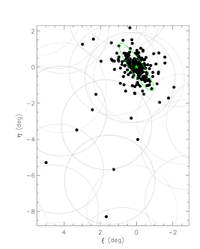
Refer to caption — Figure 1: Spatial distribution of our sample of star clusters in M31. The large black circles represent LAMOST spectroscopic plates observed since June 2014. The green star marks the central positions of M31. The green ellipse represents the optical disk of M31 of radius $R_{25}\,=\,95^{\prime}.3$ (de Vaucouleurs et al., 1991), with an inclination angle $i$ = 77 $\arcdeg$ and a position angle $P.A.$ = 38°(Kent, 1989). Also included in the sample is LAMOST-2, likely to be a cluster associated with M 33. It however falls outside the field plotted here.

Massive clusters in our sample are all selected from the catalog presented in Paper I, including 5 newly discovered clusters selected with the SDSS photometry, 3 newly confirmed and 298 previously known clusters from RBC. Paper I lists 296 known clusters from RBC. Since then, another two objects, B341 and B207, have also been observed with LAMOST, and they are included in the current analysis. The current sample do not include those listed in Paper I but selected from Johnson et al. (2012) since most of them are young but not so massive. All objects are observed with LAMOST between September, 2011 and June, 2014. Table 1 lists the name, position and radial velocity of all sample clusters analyzed in the current work. Their spatial distribution in the $\xi~{}-~{}\eta$ plane is shown in Fig. 1. Here $\xi$ and $\eta$ are respectively Right Ascension and Declination offsets relative to the optical centre of M31 (RA: 00^h42^m44^s.30; Dec:+41°16^′09^′′.0, from Huchra et al. 1991 and Perrett et al. 2002). The clusters distributes between the thin disk and the outer halo of M31. One cluster identified with LAMOST, LAMOST-2, falls close to M33 and has a radial velocity similar to that of M33. It is likely a halo cluster of M33 and is included in the current analysis.

2.2 LAMOST spectra

The LAMOST M31/M33 survey is a component of LSS-GAC (Liu et al., 2014, 2015; Yuan et al., 2015). The spectra were collected with nine unique but overlapping spectroscopic plates of 5^∘ in diameter (see Fig. 1). All plates were observed under dark or grey lunar conditions. Typically 2–3 exposures were made for each plate, with typical integration time per exposure between, depending on the observing conditions, 600–1200 s, 1200–1800 s and 1800–2400 s for bright (B), median (M) and faint (F) plates, respectively. Some test nights reserved for monitoring the telescope performance were also used to observe M31 and M33 plates. For most observations, the seeing varied between 3 – 4 arcsec, with a typical value of about 3.5 arcsec (Yuan et al., 2015).

The LAMOST spectra cover the wavelength range 3700–9000 Åat a resolving power of $R\sim 1800$ . Details about the observations and data reduction can be found in Paper I. The median signal-to-noise ratio (SNR) per pixel at 4750 and 7450 Å of spectra of all clusters in the current sample are respectively 14 and 37. Essentially all spectra have $\rm SNR(4750\,\AA)$ $>5$ except for spectra of 18 clusters. The latter have SNR(7450 Å) $>10$ . The spectra were first processed with the LAMOST 2-D Pipeline Version 2.6 (Luo et al., 2015). Flux calibration was carried out using the algorithm of Xiang et al. (2015b). For each plate, a number of sky fibres ( $\sim$ 20 for each of the sixteen spectrographs) were assigned, targeting blank sky areas. For the central area of M31 where the surface brightness from the host galaxy is high compared to the clusters targeted, the nearby sky fibres were used to subtract the local background of for the targets. A similar approach was adopted by Caldwell et al. (2009). Partly benefited from this, radial velocities derived from our observations for clusters falling close to the central bright bulge are in close agreement with those obtained by Caldwell et al. (2009). For objects observed multiple times with different plates, spectra with lower $\rm SNR(4750\,\AA)$ were scaled with a low-order polynomial to match the continuum level of spectrum of the highest and then all combined together, weighted by the spectral invariances. Radial velocities of the clusters were derived by matching the observed spectra with SSP models. Example spectra of several star clusters of different metallicities and ages (see §§3 and 4) are presented in Fig. 2. Note that the blue- and red-arm spectra were processed separately with the 2-D Pipeline and joined together after the flux calibration (Xiang et al., 2015b). No scaling nor shifting was performed in cases where the blue- and red-arm spectra did not have the same flux level in the overlapping wavelength region, as it was unclear whether the misalignment was caused by poor flat-fielding/flux-calibration or sky subtraction, or a combination of both. That is why spectra of some clusters show abnormal artefacts in wavelength range 5800 – 6300 Å. We have removed this part of spectra in Fig. 2 for better illustration. Finally the bright sky emission line at 5578 Å were not properly removed in spectra of some objects.

2.3 Photometric Data

Peacock et al. (2010) retrieved images of M31 star clusters and candidates from the SDSS archive and extracted $ugriz$ aperture photometric magnitudes those objects using SE $\rm{\scriptstyle XTRACTOR}$ . They present a catalog containing homogeneous $ugriz$ photometry of 572 star clusters and 373 candidates. Amongst them, 299 clusters are in our sample. Of those, 280, 289, 289, 287 and 285 are detected in $u,~{}g,~{}r,~{}i$ and $z$ bands, respectively. Six objects, including the five newly discovered clusters reported in Paper I (LAMOST-1–5) and MGC1 (Huxor et al., 2008) are not found in the Peacock et al. catalog but have been detected by SDSS. For the six objects, we adopt the Petrosian magnitudes available from the SDSS archive.

Also listed in Table 1 are $ugriz$ photometric magnitudes along with reddening values. The reddening values are taken from Kang et al. (2012), compiled from three sources: (1) Determinations available from the literature (Barmby et al. 2000; Fan et al. 2008; Caldwell et al. 2009, 2011). If more than one determinations are available, the average value is adopted; (2) For clusters that have no reddening values determinations in the literature, the median value of clusters within 2 kpc radius of the cluster of concern is adopted; and (3) For star clusters that fall beyond a galactocentric distance of 22 kpc, a foreground reddening value of $E(B-V)$ = 0.13 mag is adopted. Some of our sample clusters are not available in the compilation of Kang et al. For those objects, we calculate their reddening values following approaches (2) and (3) above.

Table 1: Optical photometry and reddening of massive star clusters observed with LAMOST

Name	R.A.	Decl.	$V_{r}$	$u$	$g$	$r$	$i$	$z$	$E(B-V)$
	(deg)	(deg)	( $\rm km\,s^{-1}$ )	(mag)	(mag)	(mag)	(mag)	(mag)	(mag)
B001-G039	9.96253	40.96963	-222 $\pm$ 150	19.39 $\pm$ 0.12	17.58 $\pm$ 0.07	16.61 $\pm$ 0.07	16.07 $\pm$ 0.07	15.70 $\pm$ 0.07	0.25
B002-G043	10.01072	41.19822	-370 $\pm$ 18	19.15 $\pm$ 0.10	17.86 $\pm$ 0.08	17.34 $\pm$ 0.07	17.06 $\pm$ 0.07	16.90 $\pm$ 0.09	0.01
B003-G045	10.03917	41.18478	-381 $\pm$ 9	19.43 $\pm$ 0.12	17.94 $\pm$ 0.09	17.36 $\pm$ 0.07	16.99 $\pm$ 0.07	16.82 $\pm$ 0.09	0.16
B004-G050	10.07462	41.37787	-381 $\pm$ 4	19.06 $\pm$ 0.10	17.40 $\pm$ 0.07	16.64 $\pm$ 0.07	16.28 $\pm$ 0.07	16.05 $\pm$ 0.07	0.13
B005-G052	10.08462	40.73287	-299 $\pm$ 2	17.86 $\pm$ 0.08	16.12 $\pm$ 0.07	15.32 $\pm$ 0.06	14.90 $\pm$ 0.06	14.62 $\pm$ 0.06	0.22
B006-G058	10.11031	41.45740	-244 $\pm$ 2	17.69 $\pm$ 0.07	15.92 $\pm$ 0.07	15.16 $\pm$ 0.06	14.79 $\pm$ 0.06	14.53 $\pm$ 0.06	0.11
B008-G060	10.12613	41.26907	-330 $\pm$ 4	19.03 $\pm$ 0.10	17.23 $\pm$ 0.08	16.47 $\pm$ 0.07	16.07 $\pm$ 0.07	15.86 $\pm$ 0.07	0.17
B010-G062	10.13154	41.23956	-195 $\pm$ 11	18.46 $\pm$ 0.09	17.04 $\pm$ 0.08	16.38 $\pm$ 0.07	16.02 $\pm$ 0.07	15.80 $\pm$ 0.07	0.20
B011-G063	10.13282	41.65474	-249 $\pm$ 8	18.42 $\pm$ 0.08	17.06 $\pm$ 0.07	16.43 $\pm$ 0.07	16.14 $\pm$ 0.07	15.97 $\pm$ 0.07	0.09
B011D	10.21508	40.73504	-538 $\pm$ 10	18.82 $\pm$ 0.09	17.87 $\pm$ 0.13	17.21 $\pm$ 0.07	16.49 $\pm$ 0.07	15.77 $\pm$ 0.07	0.28
B012-G064	10.13525	41.36226	-367 $\pm$ 4	16.76 $\pm$ 0.07	15.43 $\pm$ 0.07	14.83 $\pm$ 0.06	14.53 $\pm$ 0.06	14.36 $\pm$ 0.06	0.11
B013-G065	10.16022	41.42328	-422 $\pm$ 8	19.19 $\pm$ 0.11	17.63 $\pm$ 0.10	16.88 $\pm$ 0.07	16.46 $\pm$ 0.07	16.19 $\pm$ 0.08	0.13
…	…	…	…	…	…	…	…	…	…
KHM31-74	10.22055	40.58880	-55 $\pm$ 8	20.28 $\pm$ 0.19	18.51 $\pm$ 0.19	17.84 $\pm$ 0.08	17.51 $\pm$ 0.08	17.21 $\pm$ 0.11	0.26
LAMOST-1	12.23263	35.56682	-55 $\pm$ 2	19.24 $\pm$ 0.14	18.89 $\pm$ 0.04	18.13 $\pm$ 0.03	17.71 $\pm$ 0.04	17.56 $\pm$ 0.10	0.13
LAMOST-2	24.07521	30.27437	-175 $\pm$ 8	20.07 $\pm$ 0.26	18.64 $\pm$ 0.03	17.99 $\pm$ 0.02	17.73 $\pm$ 0.03	17.63 $\pm$ 0.08	0.13
LAMOST-3	11.18990	43.44303	-424 $\pm$ 8	19.02 $\pm$ 0.05	17.79 $\pm$ 0.01	17.21 $\pm$ 0.01	16.96 $\pm$ 0.01	16.74 $\pm$ 0.03	0.13
LAMOST-4	9.03580	39.29165	-230 $\pm$ 16	19.19 $\pm$ 0.05	17.88 $\pm$ 0.01	17.31 $\pm$ 0.01	17.05 $\pm$ 0.01	16.98 $\pm$ 0.03	0.13
LAMOST-5	14.73496	42.46061	-144 $\pm$ 4	17.66 $\pm$ 0.02	16.43 $\pm$ 0.00	15.88 $\pm$ 0.00	15.61 $\pm$ 0.00	15.36 $\pm$ 0.01	0.13
M086	11.36870	41.82488	-56 $\pm$ 10	19.70 $\pm$ 0.14	18.29 $\pm$ 0.09	17.90 $\pm$ 0.08	17.88 $\pm$ 0.10	17.70 $\pm$ 0.14	0.18
…	…	…	…	…	…	…	…	…	…

Note: This is a sample of the full table, which is available in its entirety in the electronic version of this article.

3 Metallicities

In this Section, we discuss measurement of cluster metallicities, characterised by [Fe/H]. To proceed, we first apply the full spectral fitting method. The SSP models that we adopt for the full spectral fitting span a wide range of age, from young to very old. Thus the fitting is applied to both young and old clusters in the sample. In addition, we have also measured the Lick indices from the LAMOST spectra. To obtain estimates of [Fe/H], the Lick indices are calibrated by integrated spectral indices of Milky Way (MW) GCs whose metallicities have previously been measured by high resolution spectroscopy and elemental abundance analysis of bona fide cluster member stars. The calibration implicitly assumes that all M31 and MW clusters have the same age. We have also determined the metallicities using the $\rm EZ\_Ages$ code. The code compares the measured Lick indices to those from the SSP models of Schiavon (2007). The models have ages ranging from 1 to 15 Gyr and [Fe/H] ranging from $-$ 1.3 to $+$ 0.3 dex. Thus in both cases, the method bases on Lick indices is only applicable to old (age $>1$ Gyr) clusters in our sample.

3.1 Metallicities from full spectral fitting

Comparison between the observed and template spectra has been widely used to derive stellar atmospheric parameters from large number of medium- to low-resolution spectra (e.g. LSP3, Xiang et al. 2015a; LASP, Luo et al. 2015; and references therein). More recently, the technique has become increasingly common for studying the integrated spectra of star clusters (Dias et al., 2010; Cezario et al., 2013). The method makes use of all information encoded in a spectrum, making it possible to perform analysis even at lower SNRs. In some implementations, the method is also insensitive to uncertainties in extinction correction or flux calibration. We apply this method to all star clusters in our sample. A comprehensive set of templates covering wide parameter space is of fundamental importance for the full spectral fitting. SSP models constructed from both empirical and synthetic spectral libraries have been published in the literature. In the current work, we adopt the SSP models presented by Vazdekis et al. (2010)²²2http://miles.iac.es/pages/ssp-models.php and Le Borgne et al. (2004)³³3http://www2.iap.fr/pegase/pegasehr/. Both models are based on empirical spectral libraries. The advantage of empirical libraries is that they consist of spectra of real stars. The public code ULySS (Koleva et al., 2009)⁴⁴4http://ulyss.univ-lyon1.fr/ is used for the fitting. Below we describe the two sets of SSP models and the ULySS code briefly.

Vazdekis et al. (2010) present SSP models covering optical wavelength range 3540.5 $-$ 7409.6 Å at a nominal resolution of full width at half-maximum (FWHM) of 2.3 Å. The models are based on the empirical stellar spectral library, Medium resolution INT Library of Empirical Spectra (MILES, Sánchez-Blázquez et al. 2006; Cenarro et al. 2007). The MILES template stars were selected to optimise the stellar parameter coverage required for population synthesis modelling. The stellar spectra were carefully flux-calibrated to an accuracy of a few per cent. Xiang et al. (2015a) use the MILES library for LSS-GAC stellar parameter determinations. The SSP models of Vazdekis et al. (2010) are using the solar-scaled theoretical isochrones of Girardi et al. (2000). Parameters of the isochrones, $T_{\rm eff}$ , log $\,g$ and [Fe/H], are transformed to the observational space by means of empirical relations between colors and stellar parameters. Seven initial mass functions (IMFs) are used. In the current work, we adopt models calculated with the Salpeter (1955) IMF. The models cover ages of $10^{8}<t<1.5\times 10^{10}$ Gyr for a metallicity range from super-solar [M/H] = $+$ 0.22 dex (Z=0.03) to [M/H] = $-$ 2.32 dex (Z=0.0004). Note that in the current, [M/H] and [Fe/H] are treated as interchangeable.

Le Borgne et al. (2004) present SSP models PEGASE-HR covering wavelength range 4000 $-$ 6800 Åat a resolution of FWHM $\sim$ 0.55 Å. The models are constructed using the empirical spectral library ELODIE (Prugniel & Soubiran, 2001; Prugniel et al., 2007). ELODIE spectra were collected using an echelle spectrograph with a very high spectral resolution ( $R~{}\sim$ 42, 000). Luo et al. (2015) adopted the library for LAMOST stellar parameters determinations. Le Borgne et al. (2004) use the spectrophotometric model of galaxy evolution PEGASE.2 (Fioc & Rocca-Volmerange, 1997) to construct the SSP models. Two different initial mass functions (IMFs) are used. In the current work, we adopt PEGASE-HR models calculated with the Salpeter (1955) IMF. The models covers ages $10^{7}<t<1.5\times 10^{10}$ Gyr for a metallicity range from [Fe/H] = $-$ 2.0 dex (Z=0.0004) to [Fe/H] = $+$ 0.4 dex (Z=0.05).

The full spectral fitting code ULySS (Koleva et al., 2009) is adopted to fit the LAMOST spectra of M31 star clusters with SSP models. ULySS is an open-source package that fits spectroscopic observations against a model through a non-linear least-squares minimisation. The model is expressed as a linear combination of non-linear components convolved with a line-of-sight velocity distribution and multiplied by a polynomial continuum. ULySS performs spectral fitting in two astrophysical contexts: the determination of stellar atmospheric parameters and the study of stellar populations of galaxies and star clusters. In the current work, we use the set of routines for stellar population study. The code is written in the GDL/IDL language. In contrast to other stellar analysis programs that require the observed spectrum to be normalized to a pseudo-continuum as a prerequisite, ULySS determines the normalization in the fitting process, by introducing a multiplicative polynomial for the scaling of model spectra. Therefore, ULySS is relatively insensitive to uncertainties in flux calibration, extinction correction, or any other sources of error that affect the shape of the observed spectrum. We run ULySS with its global minimisation option. The wavelength range adopted for the fitting has some impact on the results. After some tests, we decide to use the wavelength range 4000 $-$ 5400 Å (similar to that used by of Alves-Brito et al. 2009 and Cezario et al. 2013) for clusters with a spectra $\rm SNR(4750\,\AA)$ $>$ 5 and 6100 $-$ 6800 Å for clusters with a $\rm SNR(4750\,\AA)$ $<$ 5 but with a $\rm SNR(7450\,\AA)$ $>$ 10.

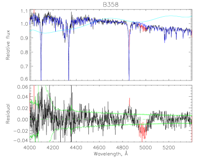
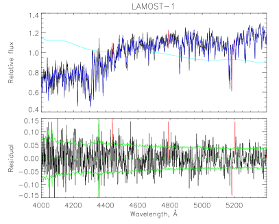
Ages and metallicities derived with ULySS are presented in Table 3. For illustration, Fig. 3 shows the fits of two example clusters, B358 a metal-poor and relatively young cluster and LAMOST-1, a metal-rich and very old cluster. The model spectra shown in the Figure are those from Vazdekis et al. Owing to the overlapping of Field of View (FoV) of adjacent plates, and some repeated observations, either because the first observations failed to pass the quality control (60% of the targets pass the SNR requirement, SNR(4750Å) or SNR(7450Å) $>10$ ) or some other reasons, over half clusters in our sample were observed more than once with LAMOST (c.f. Liu et al. 2014; Yuan et al. 2015 and Paper I). Those multi-epoch duplicate observations of the same targets provide an opportunity to test the precision of parameters yielded by the full spectral fitting method. Fig. 4 shows the distribution of differences of metallicities deduced from the duplicate observations of the same targets. Only results based on SSP models of the Vazdekis et al. are shown because those from the PEGASE-HR models are quite similar. In general, the Figure shows that metallicities yielded by full spectral fitting have a precision better than $\sim$ 0.1 dex.

Many clusters in our sample have previously been studied, some by fitting the color-magnitude diagrams (CMDs) with isochrones while others using spectral indices. We will compare our results with those in the literature in §3.3. The top left panel of Fig. 5 compares metallicities derived with ULySS but using different SSP models. Overall, the agreement is good. For clusters of metallicities [Fe/H] $>-1.0$ dex, the values derived using the PEGASE-HR models are slightly higher ( $\sim$ 0.07 dex) than those from the models of Vazdekis et al. models. For some clusters, the differences are quite significant. Most of these clusters have ages smaller than 2 Gyr (see §3.3). Excluding those outliers, the dispersion of the differences is very small ( $\sim$ 0.1 dex).

3.2 Metallicities from the Lick Indices

Table 2: Zero points to convert our measurements of equivalent widths to the Lick system from literature.

Index	Mg₂	Mg $b$	Fe5270	Fe5335	H $\beta$
Zero point^a (Å)	0.01	$-$ 0.18	$-$ 0.04	0.20	0.10
rms^a (Å)	0.03	0.56	0.55	0.59	0.59
Zero point^b (Å)	0.02	$-$ 0.14	$-$ 0.11	0.07	0.10
rms^b (Å)	0.04	0.46	0.07	0.46	0.31

^a Zero point= $I_{\rm G09}-I_{\rm thiswork}$ .

^b Zero point= $I_{\rm S12}-I_{\rm thiswork}$ .

Lick indices have been widely used for over a decade for determining ages and metallicities of star clusters. We calculate line indices in the Lick/IDS system (e.g. Worthey et al. 1994 and references therein) for old clusters with LAMOST spectral $\rm SNR(4750\,\AA)$ $>$ 10 in our sample. The observed spectra are shifted to rest frame wavelengths such that a consistent set of wavelengths can be used to define and calculate line indices. To measure the line indices, we use the code $\rm{\sc lick_{e}w}$ that comes with the $\rm EZ\_Ages$ package (Graves & Schiavon, 2008). The LAMOST spectra were smoothed to match the (lower) Lick/IDS resolution (Worthey & Ottaviani, 1997). The equivalent widths (EWs) were then measured adopting the passbands defined by Worthey et al. (1994) and Worthey & Ottaviani (1997). Values of metallicity [Fe/H] of old clusters in our sample can then be derived from the line measured indices using the empirical relations. For the latter, Galleti et al. (2009) have recently derived a new relation between [Fe/H] and [MgFe], where ${\rm[MgFe]}$ $\equiv{\rm\sqrt{{\rm Mgb\cdot\langle Fe\rangle}}}$ , and ${\rm\langle Fe\rangle}$ =(Fe5270+Fe5335)/2 (González, 1993). The relation is based on well-studied Galactic GCs supplemented by theoretical models for $-$ 0.2 $\leq$ [Fe/H] $≤\leq$ $+$ 0.5 dex,

\displaystyle{\rm[Fe/H]_{[MgFe]}}={\rm-2.563+1.119[MgFe]-0.106[MgFe]^{2}}.

For prudence, the application of the relation should be limited to clusters of ages older than 7 $-$ 8 Gyr (see Galleti et al. 2009). Alternatively, Caldwell et al. (2011) estimate metallicities of M31 GCs based on ${\rm\langle Fe\rangle}$ , again calibrated using measurements of metallicity [Fe/H] of Galactic GCs,

	$\displaystyle{\rm[Fe/H]_{\langle Fe\rangle}}=-2.23+0.83{\rm\langle Fe\rangle;~{}for~{}\langle Fe\rangle>0.9};$
	$\displaystyle{\rm[Fe/H]_{\langle Fe\rangle}}=-3.18+1.88{\rm\langle Fe\rangle;~{}for~{}\langle Fe\rangle􏰏\leq 0.9}.$

Both calibrations assume that GCs of M31 have similar ages, ignoring the fact that clusters in each of the two galaxies actually span a range of ages and the age distribution can be quite different. In the current work, we calculate metallicities of clusters in our sample using both relations. In doing so, the instrumental EWs are converted to the corresponding Lick/IDS indices using zero points derived from objects in our sample that are in common with those in the literature (Galleti et al. 2009 for the relation of Galleti et al. 2009; and Schiavon et al. 2012 for both the relations of Caldwell et al. 2011 and that adopted in the code $\rm EZ\_Ages$ ). We concentrate on a few lines indices including Mg₂, Mgb, Fe5270, Fe5335 and H $\beta$ . The zero points are determined by the averages of differences between our measurements and those from the literature. They are listed in Table 2, together with the rms of the differences.

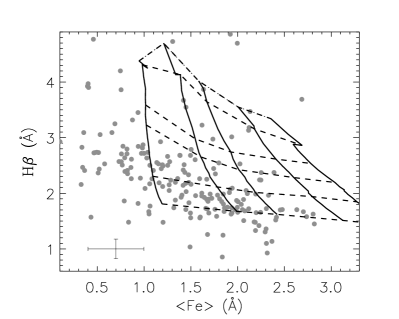
Ages and metallicities of clusters in M31 can also be determined from the Lick indices using code $\rm EZ\_Ages$ , developed by Graves & Schiavon (2008) for automatic stellar population analysis. $\rm EZ\_Ages$ is a package written in IDL that computes the mean, light-weighted age, metallicity [Fe/H], and elemental abundances [Mg/Fe], [C/Fe], [N/Fe], and [Ca/Fe] for unresolved stellar populations. This is accomplished by comparing the measured Lick indices with predictions of SSP models of Schiavon (2007), using a method described in Graves & Schiavon (2008). The method has been successfully tested by applying to Galactic GCs of known ages and chemical composition. Ages and abundances are determined by using the index-index model grids. In the current work, we use the H $\beta$ – ${\rm\langle Fe\rangle}$ index pair. The pair provide good estimates of metallicities and ages of star clusters. In additional the H $\beta$ and ${\rm\langle Fe\rangle}$ indices are relatively easy to measure and are insensitive to elemental abundance variations. Fig. 6 plots the ${\rm\langle Fe\rangle}$ – H $\beta$ grid, with our measurements of M31 clusters overplotted. There are a relatively large fraction of objects located outside the model grid. Some of them are metal poor clusters. They have blue horizontal branch stars which may not be represented in the Schiavon (2007) models. The young clusters are not included in the model, either. In addition, there are some old clusters whose H $\beta$ line indexes are so small that they fall below the predicted values of the oldest models. Most of them are actually consistent with the models if we consider the index measurement errors. A minority of them falls far away from the oldest models and that could not be caused by the measurement uncertainties alone. In those cases, the discrepancies may be partly caused by the model zero-point uncertainties (Schiavon et al., 2002) and the contaminations of Balmer lines from the evolved giants and/or intra-cluster medium (Poole et al., 2010; Caldwell et al., 2011). $\rm EZ\_Ages$ does not deal with model extrapolation, so clusters with line index measurements falling outside the model grid are excluded from the analysis. This includes clusters of metallicities [Fe/H] $<-$ 1.3 or [Fe/H] $>+0.2$ dex.

Fig. 5 compares values of [Fe/H] estimated from our spectra using various methods described above. Overall the agreement is good, with negligible offsets and small dispersions. The rms differences of values derived with ULySS using the SSP models of Vazdekis et al. and those from the relation of Galleti et al. (2009) is 0.22 dex. The corresponding value between results derived from relation of Galleti et al. (2009) and those from relation of Caldwell et al. (2011) is 0.25 dex, and 0.13 dex between the results derived from the relation of Caldwell et al. (2011) and those yielded by code $\rm EZ\_Ages$ .

3.3 Comparison with previous [Fe/H] measurements

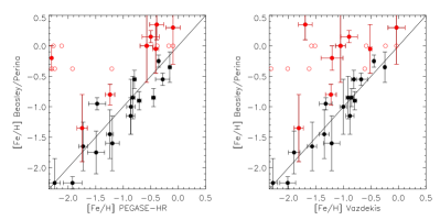
Only a few studies on the metallicity of young clusters in M31 is available in the literature. Based on high-quality spectra, Beasley et al. (2004) obtain metallicities for 30 star clusters in M31. Eight of them are young clusters. Perina et al. (2010) derive ages and metallicities of 25 young clusters by fitting the optical color-magnitude diagrams with theoretical isochrones using HST/WFPC2 data. Fig. 7 compares our metallicities derived from full spectral fitting using various SSP models and those of Beasley et al. (2004) and Perina et al. (2010). For the young clusters, except for a few outliers, our estimates, deduced using PEGASE-HR models or those of Vazdekis et al. regardless, correlate well with those obtained by Beasley et al. (2004) but with values $\sim 0.45$ dex systematically lower. Similarly, our estimates are systematically lower than those of Perina et al. (2010). Note that the latter have only two distinct values, either of ${\rm Fe/H]}=-0.38$ dex (Z $=0.008$ ) or ${\rm Fe/H]}=0.0$ dex (Z $=0.019$ , i.e. Solar). The systematics could be due to incorrect zero-point shifts applied to our estimates. Nevertheless, Fig. 7 shows that we may have significantly underestimated the metallicities of young clusters. A close scrutiny of Fig. 7 also indicates that our estimates of [Fe/H] using the PEGASE-HR models are in slightly better agreement with those of Beasley et al. than those using the SSP models of Vazdekis et al. One possible explanation is that the SSP models of Vazdekis et al. contain few templates of very young clusters. The lower age limit of templates of Vazdekis et al. is 0.063 Gyr, while many of the clusters in comparison here have ages less than 0.03 Gyr according to the determinations of Beasley et al. (2004).

Many more studies for old cluster are available in the literature and we compare our results with previous ones below. However, for completeness, old clusters analyzed by Beaslet et al. (2004) are also show in Fig. 7. The agreement with our values is excellent, except that our values derived using the PEGASE-HR models are slightly lower than those of Beasley et al.

Now we compare our results for old clusters in M31 with those in the literature. For those old clusters our results derived with various methods using different SSP models are in good agreement. Because of this, only values derived from the full spectral fitting using the PEGASE-HR models are compared to those in the literature. The comparisons are presented in Fig. 8.

We first compare our [Fe/H] values with those obtained from low- and medium- resolution spectroscopy in the literature, i.e. those of Perrett et al. (2002); Galleti et al. (2009); Caldwell et al. (2011) and Cezario et al. (2013). In general, the agreement is good. Caldwell et al. (2011) estimated metallicities from spectra obtained with the 6.5 m MMT Hectospec multi-fiber spectrograph. 45 objects of their targets are in common with ours. The differences between our and their estimates have a small rms scatter of 0.16 dex and a negligible offset of $-$ 0.02 dex. The rms scatters of differences between our results and those of Galleti et al. (2009) and Cezario et al. (2013) are slightly larger. Note, however, that the objects in common here cover a wider metallicity range than those in common with the sample of Caldwell et al. ⁵⁵5We have used the metallicities derived from the $\rm EZ\_Ages$ analysis in Caldwell et al. (2011). Their metallicities, derived from a Lick index relation using measurements of metallicity [Fe/H] of Galactic GCs,, did cover the entire metallicity range, unlike the case for the $\rm EZ\_Ages$ values., down to as low as $\sim-2$ dex. Galleti et al. (2009) present metallicity estimates based on the Lick indices for 245 GCs in M31, 144 objects of them are in common with our sample. The rms scatter of the differences between the two sets of measurements is considerable, about 0.31 dex. The overall agreement is however very good, with no obvious systematics over a wide metallicity range. The average difference between the two sets of measurements amounts to only $-0.02$ dex. Cezario et al. (2013) derive spectroscopic metallicities of 38 M31 GCs by full spectral fitting. For the 27 objects in common with ours, the differences between their and our metallicity estimates have a mean of $-$ 0.23 dex with a rms scatter of 0.38 dex. Perrett et al. (2002) present spectroscopic metallicities of about 200 GCs in M31, derived from the Lick indices. For the 93 objects in common with ours, again covering a wide range of metallicities, the differences of their and our estimates have a mean of 0.26 dex and a rms scatter of 0.47 dex. Parts of the large discrepancies between our results and those of Perrett et al. (2002) might be caused by improper background subtraction in their work for clusters near the centre of M31 where the background emission from the host galaxy is high.

Probably the most robust metallicity estimates available hitherto for star clusters in M31 are those derived from the CMDs of the individual clusters based on the mean colors of giant branch stars (Rich et al., 2005; Fuentes-Carrera et al., 2008; Perina et al., 2009; Caldwell et al., 2011) and those determined from Fe i lines detected in high-resolution (R $\sim$ 20,000) spectra (Colucci et al., 2009, 2014; Sakari et al., 2015). The giant branch stars of star clusters in M31 can be resolved by HST imaging photometry. We have collected metallicities derived from the CMDs of red giant branch stars in the literature and found 18 clusters in common with our sample (cf. middle panel of top row of Fig. 8). The objects come from Rich et al. (2005); Fuentes-Carrera et al. (2008); Perina et al. (2009) and Caldwell et al. (2011). Metallicities based on high-resolution spectroscopy are collected from Colucci et al. (2009) and Colucci et al. (2014). In total 24 objects in common with our sample are found (cf. right panel of top row of Fig. 8). Fig. 8 shows surprisingly good agreements for both comparisons. Our measurements, compared to those derived from the CMDs and from high-resolution spectroscopy, have an average difference of only 0.11 and $-$ 0.01 dex, respectively, along with a rms scatter of 0.26 and 0.16 dex, respectively.

4 Ages

4.1 Ages from LAMOST spectra

In the process of fitting the full spectrum using the ULySS code or comparing the measured Lick line indices with the predictions of SSP models using the $\rm EZ\_Ages$ code, the best-fitted age of cluster is also determined simultaneously with the metallicity. Ages of clusters thus derived with ULySS and $\rm EZ\_Ages$ are listed in Table 2.

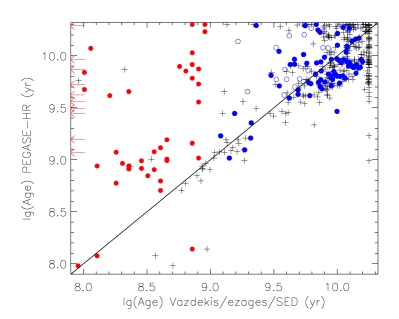
We first test the precision of ages delivered by full spectral fitting for clusters with duplicate observations. Fig. 9 shows that a precision of better than 2 Gyr has been achieved for most clusters. Fig. 10 compares ages determined with the PEGASE-HR models and those with the models of Vazdekis et al. In general, ages derived with the two sets of SSP models are consistent with each other. No obvious systematic offset is seen. The scatters of their differences are however considerable. We notice that some clusters of PEGASE-HR ages between $\sim$ 3 and $\sim$ 15 Gyr are all found to have an age of $\sim$ 15 Gyr as derived with models of the Vazdekis et al., i.e. the upper age limit of the models of Vazdekis et al. On the other hand, ages of those clusters returned by the $\rm EZ\_Ages$ code are consistent with the PEGASE-HR ages. It seems that the full spectral fitting with the models of Vazdekis et al. may have overestimated the ages of some clusters, by returning an age of 15 Gyr for those clusters, the upper limit of age of the models.

The code $\rm EZ\_Ages$ only provide parameters for clusters falling within the model grids, as Fig. 6 shows. This yields ages of 103 old clusters in our sample. The results are compared with those yielded by ULySS fitting with the PEGASE-HR models in Fig. 10. The agreement is good overall, with a negligible average offset of $\sim$ 1 Gyr. Note that ages yielded by $\rm EZ\_Ages$ are based on the H $\beta$ index only. The Padova isochrones, adopted in the models of Schiavon (2007) and used in Caldwell et al. (2011), do not contain blue horizontal branch (HB) stars. Because an actual metal-poor cluster with a blue HB tends to have stronger Balmer lines than predicted by Padova models of the same age and metallicity, cluster ages yielded by EZ Ages tend to be underestimated for metal poor clusters. This effect can be clearly seen in Fig. 10, where $\rm EZ\_Ages$ ages of clusters of [Fe/H] $􏰍<-0.95$ dex are all smaller than those derived with ULySS with the PEGASE-HR models. If we exclude those clusters of [Fe/H] $􏰍<-0.95$ dex, then no obvious systematic offset is seen between the $\rm EZ\_Ages$ and PEGASE-HR ages.

4.2 Ages from SED fitting

Ages of young clusters can be estimated by SED fitting of multi-band photometry (Wang et al., 2010; Fan et al., 2010; Kang et al., 2012, and references therein). We have collected magnitudes in $ugriz$ passbands for clusters in our sample (see Sect. 2.3). With photometric data from the optical to the NIR, we are able to break the age-metallicity degeneracy of young clusters (Anders et al., 2004). The photometric data are de-reddened using reddening values described in §2.3 and the reddening law of Yuan et al. (2013). The de-reddened data are then fitted with predictions of the SSP models to determine the ages. The SSP models of Bruzual & Charlot (2003, hereafer BC03)⁶⁶6http://www2.iap.fr/users/charlot/bc2003/ are adopted. BC03 models are constructed using various stellar libraries and IMFs. In this work we adopt those models of IMF from Chabrier (2001) and stellar library from the Padova isochrones. The models cover ages of $5.0<{\rm log}\,t<10.3$ (yr), with log $t$ bins ranging from 0.005 to 0.05 (yr). The models have six metallicities (of values of Z of 0.0001, 0.0004, 0.004, 0.008, 0.02 and 0.05).

The SED fitting is applied to all sample star clusters that are detected in at least four bands. For each object, we select BC03 model of metallicity closest to that derived for that object with full spectral fitting. The age is then determined by minimising $\chi^{2}$ defined as,

\chi^{2}=\sum\frac{(m^{\rm obs}_{\lambda i}-m^{\rm mod}_{\lambda i}(t))^{2}}{\sigma_{\lambda i}^{2}},

(1)

where $m^{\rm obs}_{\lambda i}$ and $m^{\rm mod}_{\lambda i}$ are the observed and model magnitudes in band $\lambda i=u,~{}g,~{}r,~{}i$ or $z$ ; and $\sigma_{\lambda i}$ is the uncertainty of magnitudes in band $\lambda i$ . The uncertainty include the contributions from observed and model magnitudes as well as from the error of distance modulus (Ma et al., 2012), i.e., $\sigma^{2}_{\lambda i}=\sigma^{2}_{{\rm obs},\lambda i}+\sigma^{2}_{{\rm mod},\lambda i}+\sigma^{2}_{{\rm dm},\lambda i}$ . Note that $\sigma_{{\rm mod},\lambda i}$ and $\sigma_{{\rm dm},\lambda i}$ only affect the absolute value of $\chi^{2}$ but not the best-fit result. 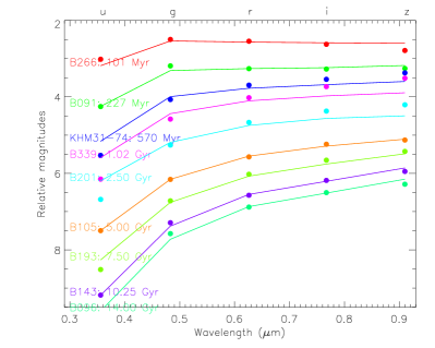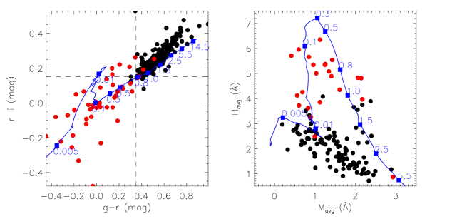In the current work, we have assumed $\sigma_{{\rm mod},\lambda i}=0.05$ mag and $\sigma_{{\rm dm},\lambda i}=0.07$ mag.

Ages of 292 clusters in our sample are obtained with the SED fitting. They are listed in Table 3. Examples of best-fits for nine objects are plotted in Fig.11. Fig.11 shows that the SEDs of old clusters have similar shapes that are hard to distinguish. Thus the SED best-fit ages are only adopted for young clusters. In total there are 46 young clusters with best-fit SED ages $t\leq$ 1 Gyr in our sample. The left panel of Fig. 12 plots the dereddened $g-r$ versus $r-i$ color-color diagram of all clusters in our sample. Young and old clusters are well separated in color $g-r$ , with young ones having $g-r<0.35$ mag. This is consistent with the color criteria ( $g-r<0.3$ mag) that Peacock et al. (2010) used to select young clusters. The cut between young and old clusters in color $r-i$ is less clear. A roughly border line is $r-i=0.15$ mag, although there are young and old clusters on both side of the line. In the right panel of Fig. 12 we present a plot of the average Balmer line index H_avg versus the average metal line index M_avg measured from the LAMOST spectra of clusters with a $\rm SNR(4750\,\AA)$ $>$ 10 in our sample. The indexes are defined as $\rm M_{avg}=(Fe5270+Mgb)/2$ and $\rm H_{avg}=(H\delta F+H\gamma F+H\beta)/3$ , respectively. Except for B016, all young clusters identified by SED fitting fall around the sequence line for young clusters. For B016 the SED fitting yields log $t=8.9\pm 0.2$ (yr), significantly younger than log $t=10\pm 0.2$ (yr) given by full spectral fitting. The latter is consistent with the estimate of Caldwell et al. (2011), log $t=10$ (yr). The age of B016 from SED fitting might have been underestimated but the value is still consistent with that from the full spectral fitting considering the uncertainties of both estimates.

Ages derived from the various approaches have already been compared in Fig. 10, including those from the SED fitting for young clusters. The scatters are significant. Ages derived from full spectral fitting are systematically older than those from SED fitting. Some of the young clusters identified by SED fitting have very old ages, $3-15$ Gyr, from full spectral fitting. Such old ages are inconsistent with the colors and Balmer/metal line indices of those young clusters. We believe that full spectral fitting may have overestimated the ages of young clusters.

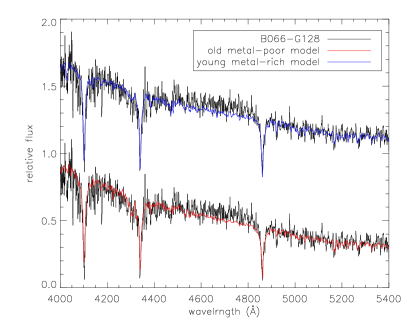
We have checked carefully the spectra of those young clusters as well as those of both the PEGASE-HR and Vazdekis et al. models. The young clusters are found to have strong Balmer lines and weak metal lines (such as Mgb line). They can be fitted by not only young and metal-rich SSP models, but also old and metal-poor models. An example is shown in Fig. 13. B066 is a young cluster, with $t$ = 0.72 Gyr from the SED fitting method in the current work and $t$ = 0.71 Gyr from Perina et al. (2010). The metallicity of B066 is 0.0 dex from Perina et al. (2010). Yet the full spectral fitting method gives values of [Fe/H] = $-$ 2.12 and $-$ 1.52 dex and $t$ = 1.17 and 1.07 Gyr from PEGASE-HR and Vazdekis et al. models, respectively. Both the old, metal-poor model and the young, metal-rich model fit well with the observed spectra of B066. Thus there is degeneracy when we use the full spectral fitting method. In most cases, young clusters have been assigned old ages along with poor metallicities, such as VDB0, B448, B342 and B066, etc. Both ages and metallicities of these clusters obtained from the full spectral fitting are problematic. For these clusters we adopt only the ages from SED fitting and simply assigned their metallicities as 0.0 dex. We have also found two opposite cases (B074 and B013). They are old, metal-poor clusters, but have been assigned a young age and a high metallicity based on the full spectral fitting method. B074 is misclassified by the Vazdekis et al. models, but correctly classified by the PEGASE-HR models. B013 is misclassified by the PEGASE-HR models but correctly classified by the Vazdekis et al. models. The abnormal results of these two clusters are excluded in Table 3.

4.3 Comparison with previous age estimates

Ages of old clusters derived from the full spectral fitting with the PEGASE-HR models are in good agreement with those from $\rm EZ\_Ages$ , while the PEGASE-HR ages for young clusters are probably overestimated. For the purpose of comparisons with previous work, we have adopted the PEGASE-HR ages for old clusters in our sample, while for young clusters the ages from SED fitting are used when available. Note that due to lack of suitable photometric data, SED fitting does not provide ages for all young clusters in the sample. The number of young clusters without a SED fitting age is however small ( $\leq$ 5). For those a couple of clusters, their ages yielded by full spectral fitting may have been overestimated (see Fig. 14).

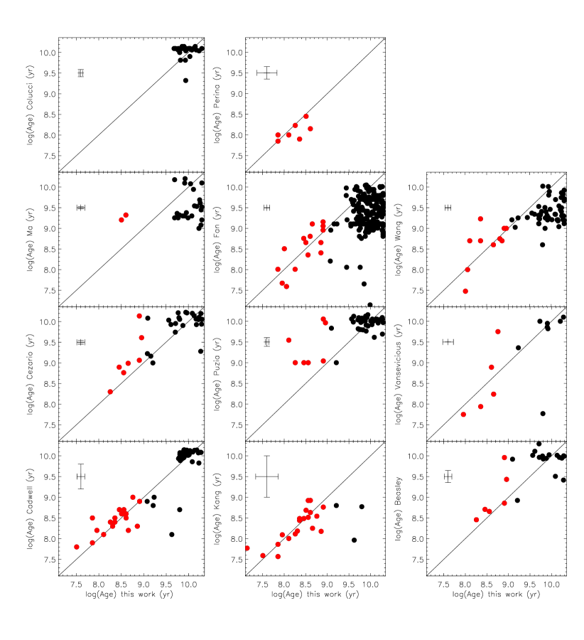
In Fig. 14, we compare our ages with those in the literature, Beasley et al. (2004), Perina et al. (2010), Puzia et al. (2005), Vansevičius et al. (2009), Caldwell et al. (2009, 2011), Colucci et al. (2009), Colucci et al. (2014), Ma et al. (2009, 2011), Ma (2012), Wang et al. (2010), Fan et al. (2010), Kang et al. (2012) and Cezario et al. (2013). Beasley et al. (2004) derive ages of 30 clusters in M31 from spectral indices. 24 of them are in common with our sample. Their results are very similar with ours. The scatter is small. Puzia et al. (2005) present ages of 70 GCs of M31 from the Lick line indices. 50 of them are found in our sample. In general the agreement between our age estimates and theirs is good, except for 6 young clusters. Considering the SSP models used by Puzia et al. (2005) do not cover ages younger than $1$ Gyr, their estimates for young clusters may be incorrect. Vansevičius et al. (2009) derive ages of 238 high probability star cluster candidates in M31 selected based on multi-band photometric data and images. 17 of them are included in our sample. Our results are consistent with theirs, except for one GC, B384, for which we derive an age of log $t=9.8$ (yr) while Vansevičius et al. (2009) give a result of log $t$ =7.77 (yr). Our result is consistent with that of Caldwell et al. (2011) who find log $\,t=10.1$ (yr). Caldwell et al. (2009) estimate ages of young clusters from spectral indices and Caldwell et al. (2011) derive ages of old clusters from spectra indices using $\rm EZ\_Ages$ . 73 objects are common between our sample and those of Caldwell et al. (2009, 2011). The agreement between our and their estimates is very good. The ages of old clusters from Caldwell et al. (2011) are slightly larger than our results. This could be caused by the different SSP models used to calculate the ages. Note that Caldwell et al. (2011) simply assign an age of 14 Gyr to all clusters of [Fe/H] $<-$ 0.95 dex. This may not only lead to overestimated ages, but also masses of some clusters (see §5). Our ages of five clusters (B124, B338, B119, B106 and B365) found to be young by Caldwell et al. (2009) are overestimated. The differences for three of them (B124, B119 and B106) are however quite small, in fact consistent within the error bars. The differences for the other two objects (B338 and B365) are slightly larger. Both clusters are also found to be young by Kang et al. (2012), who estimate ages of 182 young clusters by SED fitting of multi-band photometric data. A comparison of our age estimates and those of Kang et al. (2012) is also presented in Fig. 14. The agreement is good except for B338 and B365. Cezario et al. (2013) derive ages by full spectral fitting using code ULySS and SSP models of Vazdekis et al. For old clusters it is not surprisingly that their results are in good agreement with ours. For young clusters, the estimates of Cezario et al. (2013), as those of ours based on full spectral fitting, are systematically higher than our values derived from SED fitting and adopted here. Perina et al. (2010) estimate ages of some young clusters by comparing model isochrones in CMDs with data obtained from the HST/WFPC2 observations. 7 objects are in common with our sample and the agreement is again good. Colucci et al. (2009) and Colucci et al. (2014) determine ages for some star clusters with high-resolution spectroscopy. 24 objects studied by them are included in our sample. The comparison shows that our estimates are consistent with results from high-resolution spectroscopy. Ma et al. (2009, 2011); Wang et al. (2010) and Fan et al. (2010) estimate ages of M31 star clusters by SED fitting of multi-band photometric measurements. For young clusters, their results are consistent with ours. However, their estimates of old clusters are systematically smaller than ours. The discrepancies are significant. As discussed above, the SED fitting may not be suitable for determining ages of old clusters.

5 Masses

Once the age and metallicity of a star cluster have been determined, its mass can be estimated by comparing the photometric measurements with the SSP models. In the current work, we use the SDSS optical $ugriz$ photometry and the BC03 models for the purpose. The BC03 models are normalized to one Solar mass in stars of age $t$ =0 Gyr. Thus the mass of a cluster can be estimated by the difference between the observed intrinsic absolute magnitude and that predicted by the models in $ugriz$ bands. To calculate the intrinsic absolute magnitudes of clusters in our sample, we use the reddening values described in §2.3 and listed in Table 1. The distance modulus of M31 is taken to be $(m-M)_{0}$ = 24.43 mag (Caldwell et al., 2011). Clusters metallicities derived from full spectral fitting with the PEGASE-HR models are adopted when calculating the masses. As for the ages, again those yielded by the PEGASE-HR models are adopted except for young clusters for which the ages from SED fitting are used when available.

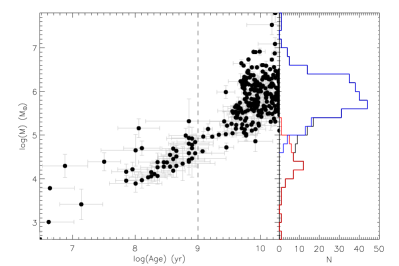
With this approach, we have been able to determine masses of 295 clusters in our sample. The results are listed in Table 3. In Column ‘Note’ of Table 3, the method used to derive the ages adopted for calculating the mass is marked, where values 1 and 2 refer to PEGASE-HR and SED fitting ages, respectively. The masses thus estimated for our M31 sample clusters are plotted against age in Fig. 15. The estimated masses span a range from $\sim 10^{3}$ to $\sim 10^{7}{\rm M_{\odot}}$ . Two discrete peaks are seen in the cluster mass histogram distribution, at $10^{4.3}$ and $10^{5.7}\,{\rm M_{\odot}}$ , produced by young and old clusters in the sample, respectively.

We compare in Fig. 16 our mass estimates to determinations in the literature (Barmby et al. 2007, 2009; Caldwell et al. 2009, 2011; Strader et al. 2011; Ma et al. 2015). The masses presented in Barmby et al. (2007, 2009), Caldwell et al. (2009, 2011) and Ma et al. (2015) are all estimated by adopting certain values of mass-to-light ratio $M/L$ . Barmby et al. (2007, 2009) and Ma et al. (2015) use $M/L$ ratios given by the SSP models as in the case of the current work. Caldwell et al. (2011) assume constant ratio of $M/L_{V}=2$ . In contrast, the masses presented in Strader et al. (2011) are estimated from the velocity dispersions and structural parameters of the star clusters. Overall, our mass estimates are in good agreement with determinations presented in those studies. For old ( $t>1$ Gyr) or massive ( $M>10^{5}\,{\rm M_{\odot}}$ ) clusters our mass estimates are slightly larger than the previous determinations. This is probably caused by the different SSP models used. The fact that both Caldwell et al. (2011) and Ma et al. (2015) calculated the cluster masses using the ages of Caldwell et al. (2011), which are slightly higher than our values (see §4.3), may also partly be responsible for the discrepancies.

Table 3: Derived properties of star clusters in our sample.

Name	[Fe/H]^a	[Fe/H]^b	[Fe/H]^c	[Fe/H]^d	[Fe/H]^e	log $t$ ^f	log $t$ ^g	log $t$ ^h	log $t$ ⁱ	Note^j	log $M$
	(dex)	(dex)	(dex)	(dex)	(dex)	(yr)	(yr)	(yr)	(yr)		( $\rm M_{\odot}$ )
B001-G039	$-0.66\pm 0.11$	$-0.84\pm 0.04$	$-0.80$	$-0.75$	$-0.88$	$9.80\pm 0.15$	$10.25\pm 0.01$	–	$9.95$	1	$5.69\pm 0.12$
B002-G043	$-2.17\pm 0.24$	$-2.32\pm 0.01$	–	–	–	$9.86\pm 0.11$	$10.05\pm 0.19$	–	–	1	$5.10\pm 0.09$
B003-G045	$-1.70\pm 0.13$	$-1.33\pm 0.15$	$-1.42$	–	–	$10.24\pm 0.05$	$9.62\pm 0.08$	–	–	1	$5.59\pm 0.04$
B004-G050	$-0.65\pm 0.06$	$-0.73\pm 0.06$	$-0.58$	$-0.71$	$-0.75$	$10.27\pm 0.02$	$10.19\pm 0.07$	–	$10.10$	1	$5.93\pm 0.02$
B005-G052	$-0.63\pm 0.04$	$-0.78\pm 0.02$	$-0.69$	$-0.63$	$-0.87$	$9.92\pm 0.06$	$10.25\pm 0.01$	–	$10.15$	1	$6.26\pm 0.05$
B006-G058	$-0.49\pm 0.04$	$-0.52\pm 0.04$	$-0.28$	$-0.41$	$-0.28$	$9.92\pm 0.06$	$10.00\pm 0.06$	–	$9.66$	1	$6.19\pm 0.05$
B008-G060	$-0.59\pm 0.09$	$-0.76\pm 0.06$	$-0.70$	$-0.73$	$-0.63$	$9.92\pm 0.13$	$10.25\pm 0.05$	–	$9.63$	1	$5.73\pm 0.11$
B010-G062	$-1.53\pm 0.15$	$-1.38\pm 0.15$	–	–	–	$9.69\pm 0.10$	$9.69\pm 0.09$	–	–	1	$5.56\pm 0.07$
B011-G063	$-1.49\pm 0.09$	$-1.37\pm 0.15$	$-1.00$	$-1.37$	$-0.95$	$10.19\pm 0.03$	$9.93\pm 0.12$	–	$9.62$	1	$5.82\pm 0.02$
B011D	$-1.17\pm 0.09$	$-1.18\pm 0.12$	$-0.91$	$-1.36$	$-0.81$	$9.62\pm 0.08$	$9.73\pm 0.12$	–	$9.58$	1	$5.40\pm 0.06$
B012-G064	$-2.02\pm 0.03$	$-1.91\pm 0.02$	$-0.16$	$-1.61$	$-0.12$	$10.08\pm 0.04$	$10.07\pm 0.04$	–	$9.52$	1	$6.40\pm 0.04$
B013-G065	–	$-0.59\pm 0.10$	–	–	–	–	$10.05\pm 0.17$	–	–	1	$5.67\pm 0.15$
…	…	…	…	…	…	…	…	…	…	…	…
KHM31-74	$-0.62\pm 0.12$	–	–	–	–	–	–	$8.76\pm 0.52$	–	2	$4.35\pm 0.39$
LAMOST-1	$-0.31\pm 0.04$	$-0.36\pm 0.03$	$-0.29$	$-0.06$	$-0.29$	$9.97\pm 0.05$	$10.16\pm 0.04$	–	$9.66$	1	$5.26\pm 0.04$
LAMOST-2	$-0.57\pm 0.08$	$-0.66\pm 0.08$	–	–	–	$10.16\pm 0.31$	$10.25\pm 0.01$	–	–	1	$5.31\pm 0.20$
LAMOST-3	$-1.58\pm 0.12$	$-1.75\pm 0.13$	$-1.54$	$-1.60$	–	$9.78\pm 0.07$	$10.07\pm 0.16$	–	–	1	$5.22\pm 0.06$
LAMOST-4	$-1.90\pm 0.20$	$-1.86\pm 0.13$	$-1.34$	$-1.45$	–	$10.30\pm 0.01$	$10.09\pm 0.16$	–	–	1	$5.61\pm 0.01$
LAMOST-5	$-2.18\pm 0.04$	$-2.17\pm 0.03$	$-2.36$	$-2.00$	–	$10.17\pm 0.03$	$9.95\pm 0.05$	–	–	1	$6.11\pm 0.02$
M086	$-0.28\pm 0.16$	–	–	–	–	–	–	$8.61\pm 0.19$	–	2	$4.18\pm 0.15$
…	…	…	…	…	…	…	…	…	…	…	…

This is a sample of the full table, which is available in its entirety in the electronic versions of this article.

^a Clusters metallicities from full spectral fitting with the PEGASE-HR models.

^b Clusters metallicities from full spectral fitting with the models of Vazdekis et al.

^c Clusters metallicities from the [MgFe] index using the relation of Galleti et al. (2009).

^d Clusters metallicities from the ${\rm\langle Fe\rangle}$ index using the relation of Caldwell et al. (2011).

^e Clusters metallicities from the $\rm EZ\_Ages$ package.

^f Cluster ages from full spectral fitting with the PEGASE-HR models.

^g Cluster ages from full spectral fitting with the models of Vazdekis et al.

^h Cluster ages from SED fitting.

ⁱ Cluster ages from the $\rm EZ\_Ages$ package.

^j Note $=$ 1: Mass estimated using the PEGASE-HR age; 2: Mass estimated using age from SED fitting.

6 Discussion

6.1 GCs in streams

The stellar halo of M31 is rich of substructures including streams, loops and filaments. Both metal rich and poor substructures are detected (e.g. Ibata et al. 2014), pointing to the presence of ongoing multiple accretion events. Many GCs found at large distances from the centre of M31 appear spatially associated with those substructures (Mackey et al., 2010). Some of those distant clusters are included in the current sample. The most intriguing case is LAMOST-1, a new identified GC with LAMOST (Paper I). It falls on the Giant Stellar Stream ( ${\rm[Fe/H]}>-0.6$ dex; Ibata et al. 2014) and has a radial velocity suggesting its association with the Stream. In the current work, we find a value of metallicity [Fe/H] $=-0.4$ dex and an age of 9.2 Gyr for LAMOST-1. LAMOST-1 is the most metal-rich of amongst the distant clusters in our sample. Its derived metallicity is compatible to that of RGB stars in the Giant Stellar Stream (Tanaka et al., 2010; Ibata et al., 2014). The deduced age of LAMOST-1 is also in good agreement with the average age of red clump (RC) stars in the Giant Stellar Stream (Brown et al., 2006; Tanaka et al., 2010). The metallicity and age derived of LAMOST-1 suggest that it probably formed in an early-type and relatively massive dwarf galaxy, of mass comparable to that of the Large Magellanic Cloud (LMC) or the Sagittarius (Sgr) dwarf spheroidal.

The other remote GCs at large distances from M31 in our sample are all very old, comparable to the age of the universe, suggesting parent galaxies formed in the early universe. Those clusters have however a range of metallicities, suggesting the variety of substructures currently being accreted into the outer halo of M31. MCGC8 is the second most metal-rich distant GC in our sample. It falls on Stream D in the halo of M31. The metallicity of MCGC8 is [Fe/H] $=-$ 1.1 dex, similar to values found for stars in the stream (Tanaka et al., 2010). It may be formed in a fairly massive galaxy, considering its metallicity. H26 falls on Stream C and has a metallicity [Fe/H] $=-1.6$ dex, again consistent with values determined for stars associated with the stream (Tanaka et al., 2010). The relatively low metallicity suggests that the stream may be the relics of an intermediate-mass dwarf galaxy. LAMOST-4 and G002 fall on ‘Association 2’, a spatial overdensity of GCs found by Mackey et al. (2010). They have very similar metallicities ([Fe/H] = $-$ 1.9 dex for LAMOST-4 and $-$ 2.1 dex for G002) and are spatially close to each other. Thus they may both come from a dwarf galaxy of a relatively low mass.

6.2 Age and metallicity distributions

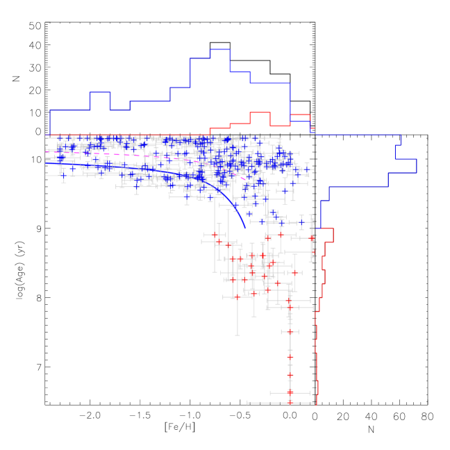
The ages derived for all clusters in our sample are plotted against metallicities in Fig. 17. Here the metallicities are those obtained from full spectral fitting with the PEGASE-HR models. For old clusters, the values are consistent with estimates derived from other methods as well as with previous determinations in the literature. For young clusters, they may have been underestimated, by less than 0.5 dex compared to those of Beasley et al. (2004) and Perina et al. (2010). Ages for most objects in the plot are again those derived with the PEGASE-HR models, except for young clusters for which the ages deduced by SED fitting are adopted when available. A small number of the young clusters have very low metallicities with [Fe/H] $<-1.0$ dex. The values may be underestimated given that the PEGASE-HR models are not suitable for young clusters, as discussed in §4.2. If we ignore those objects, then the remaining young clusters in our sample clump at the bottom right of the Figure, with similar ages around 0.3 Gyr and metallicities around $-0.3$ dex. The latter is comparable to the solar value considering that we may have underestimated the metallicities of those young clusters. The result is consistent with previously studies (e.g. Beasley et al. 2004).

Most old clusters in our sample, 240 in number, have ages larger than 4 Gyr. Only 19 have ages in the range of $1<t<4$ Gyr. The ages of old clusters peak at $t\sim$ 8 Gyr. The metallicities of Galactic GCs are known to have a bimodal Gaussian distribution, peaking at [Fe/H]= $-$ 1.60 and $-$ 0.59 dex, respectively (Harris, 1996; Galleti et al., 2009). The distribution of old clusters of M31 in our sample is quite different. It has a very broad than bimodal distribution. Again this is consistent with the findings of most previous studies (Barmby et al., 2000; Perrett et al., 2002; Lee et al., 2008; Galleti et al., 2009; Caldwell et al., 2011, and references therein). In any case, the metallicity distribution of M31 GCs resembles nothing like a single Gaussian distribution. It has an obvious broad peak around [Fe/H]= $-0.7$ dex, but also an almost flat distribution down to $\sim-2$ dex.

The old clusters in Fig. 17 can be loosely divided into three groups. The group of metallicities richer than $\sim-0.7$ dex have a wide range of ages (1–15 Gyr). Objects poorer than [Fe/H] $\sim-0.7$ dex seem to have two groups – one of the oldest ages with all values of metallicity down to $\sim-2$ dex and another with metallicity increasing with decreasing age. The later two groups are similar to those found for Galactic GCs (Marín-Franch et al., 2009; Forbes & Bridges, 2010, and references therein). Studies of Galactic GCs show that the group of GCs with very old ages and a flat age–[Fe/H] relation are probably formed in situ in a rapid enrichment process on a time-scale less than 1 Gyr. The other group of GCs with range of ages and an age–metallicity relation are probably accreted from dwarf galaxies, such as the Sgr and Canis Major (CMa) dwarf galaxies (Forbes & Bridges 2010 and references therein). The scenario may apply to M31. The difference is that those young and intermediate-age GCs in M31 are younger and more meta-rich than those found in the Milky Way, suggesting that the major accretion and merger in M31 continued several (about 4; cf. Fig. 16) Gyr even after that had ceased in the Milky Way. Most of those old, metal-rich ([Fe/H] $>~{}-$ 0.7 dex) clusters in the first group are found in the thin disk of M31 and have ages about 8–9 Gyr. These cluster may also form in a rapid enrichment process but at a later epoch than that for the old clusters found in the halo of M31.

6.3 Spatial distribution and radial metallicity gradient

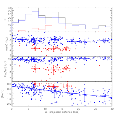
The top panel of Fig. 18 shows the distributions of de-projected distances from the centre of M31 for all, young and old clusters in our sample. The distribution of all clusters (dominated by old ones) peaks at $\sim$ 7 kpc. The distribution of young clusters is quite different. They occur from a few kpc to as far as 25 kpc. The distribution has a broad weak peak around 12 kpc. Some of these young clusters are clearly associated with the well-known star formation region, the 10 kpc “ring of fire”, in the M31 disk (Brinks & Shane, 1984; Dame et al., 1993; Pagani et al., 1999).

The lower three panels of Fig. 18 plot the masses, ages and metallicities of clusters in our sample against the de-projected distances from the centre of M31. Both ages and masses of young and old clusters have a flat distribution in distance. However, the metallicities of both old and young clusters show clear evidence of variations as a function of distance. The old clusters show a clear negative metallicity gradient, measured $\Delta{\rm[Fe/H]}/\Delta R=-0.038\pm 0.023$ dex $\rm\,kpc^{-1}$ by a linear fit to the means in the individual distance bins. This gradient is steeper than previous findings in the literature. More recently, Gregersen et al. (2015) obtain a metallicity gradient of $-0.020\pm 0.004\rm\,dex\,kpc^{-1}$ from RGB stars observed in the PHAT program. In contrast to old clusters, the metallicities of young clusters do not show clear trend of variations. Their mean metallicity first decreases from a value of $-0.2$ dex at $7$ kpc to $-$ 0.5 dex at 13 kpc but then but then flattens..

7 Summary

We select from Paper I a sample of 305 massive star clusters in M31 and one probably associated with M33 observed with LAMOST since June, 2014. From the LAMOST spectra combined with archival $ugriz$ optical photometric measurements, we present new homogeneous estimates of the metallicities, ages and masses of these clusters.

Using the full spectral fitting code ULySS in combined with different SSP models (PEGASE-HR, Vazdekis et al.), we have determined parameters including metallicities and ages of all clusters, young and old. Values derived with different SSP models are in consistent with each other for most clusters. Metallicities of young clusters estimated with the PEGASE-HR models are in better agreement with previous determinations than those estimated with the models of Vazdekis et al. In addition, ULySS fitting with the models of Vazdekis et al. may have incorrectly assigned a constant age, 15 Gyr, the upper limit of the models, to some old clusters. Thus in general, we believe that the ULySS code combined with the PEGASE-HR models work better for cluster parameter estimates than with the models of Vazdekis et al. For old ( $t>1\,$ Gyr) clusters, parameters determined with full spectral fitting are in good agreement with those derived from the Lick line indices. For young ( $t<1\,$ Gyr) clusters, the spectral fitting may have underestimated the cluster metallicities by as much as 0.5 dex and systematically overestimated the cluster ages. We apply a SED fitting method to calculate the ages of young clusters by comparing their SDSS $ugriz$ photometric data with the predictions of the BC03 models. The SED fitting is able to break the age-metallicity degeneracy. Ages of young clusters from SED fitting are in good agreement with results in the literature. Overall, among all the resultant parameters from those different methods, we prefer the metallicities from the full spectral fitting with the PEGASE-HR models for all objects in our sample. For the ages, we prefer those from the full spectral fitting with the PEGASE-HR models for old clusters and those from the multi-band SED fitting for young clusters. Based on the PEGASE-HR metallicities and ages, and the SED fitting ages for young clusters when available, we estimate the masses of 299 star clusters in our sample by comparing their photometry to the BC03 models. Our estimated metallicities, ages and masses are all in good agreement with previous determinations in general.

In our sample, we find 46 young and 260 old clusters. The masses determined range from $10^{3}$ to $10^{7}\,\rm M_{\odot}$ , peaking at $10^{4.3}\,\rm M_{\odot}$ and $10^{5.7}\,\rm M_{\odot}$ for young and old clusters, respectively. The metallicities of M31 star clusters do not show a clear bimodal nor a single Gaussian distribution. The old clusters have a peak at [Fe/H] $=-$ 0.7 dex, more metal-rich than the peak value of Galactic GCs. Young clusters have metallicities comparable to the Sun and clump in a small area to the bottom-right in the age-metallicity diagram. The old clusters in M31 seem to fall into three groups in the diagram. The first group has the oldest ages and metallicities poorer than $\sim-0.7$ dex, with no obvious age–metallicity relation. They were probably formed in situ in the halo in the early epoch of M 31 with a rapid process. The second group has metallicities also poorer than $\sim-$ 0.7 dex but shows a clear age–metallicity relation, with young clusters being more metal rich than older ones. They probably come from disrupted dwarf galaxies accreted by M31 in the past. Compared to those Milky Way GCs that are also believed to be accreted, they are younger and more metal-rich, suggesting that M31 may have been subjected to substantial merger events more recently than the Milky Way. The third group of clusters has metallicities richer than $\sim-0.7$ dex and spans a wide range of ages. A significant fraction of them has ages about 8–9 Gyr and are mainly found in the disk of M31. These clusters might also form in situ in the disk of M31, but at an epoch much later than those formed in the halo.

Most of the young clusters fall at de-projected distances between 7 and 17 kpc to the centre of M31. Young clusters found near de-projected distance of 13 kpc, probably associated with the ring structure of M31, have lower metallicities than the other young clusters. Finally, old clusters have a wide spatial distribution, peaking around 7 kpc. Those in the inner region (of de-projected distances 0 – 30 kpc) show a clear metallicity gradient of $\Delta{\rm[Fe/H]}/\Delta R=-0.038\pm 0.023$ dex $\rm\,kpc^{-1}$ .

Some of the star clusters in our sample are associated with the streams in the outer halo of M31. Among them, LAMOST-1, MCGC8 and H26 are probably associated with the Giant Stellar Stream, Stream D and Stream C, respectively. Metallicities determined for these objects in the current work are consistent with this interpretation. Most of the distant clusters in our sample are very old except for LAMOST-1, and are therefore most likely relics of early-type dwarf galaxies accreted by M31.

We want to thank the referee for detailed and constructive comments that help improve the manuscript significantly. This work is partially supported by National Key Basic Research Program of China 2014CB845700 and China Postdoctoral Science Foundation 2014M560843. The LAMOST FELLOWSHIP is supported by Special Funding for Advanced Users, budgeted and administrated by Center for Astronomical Mega-Science, Chinese Academy of Sciences (CAMS). B.Q.C thanks Professor Jun Ma for very useful comments. Z.F. is supported by the National Natural Science Foundation of China (NFSC) 11373003 and National Key Basic Research Program of China (973 Program) No. 2015CB857002. G.C.L. is supported by the National Natural Science Foundation of China (NFSC) 11303020. This work has made use of data products from the Guoshoujing Telescope (the Large Sky Area Multi-Object Fibre Spectroscopic Telescope, LAMOST). LAMOST is a National Major Scientific Project built by the Chinese Academy of Sciences. Funding for the project has been provided by the National Development and Reform Commission. LAMOST is operated and managed by the National Astronomical Observatories, Chinese Academy of Sciences. Funding for SDSS-III has been provided by the Alfred P. Sloan Foundation, the Participating Institutions, the National Science Foundation, and the U.S. Department of Energy Office of Science. The SDSS-III web site is http://www.sdss3.org/. SDSS-III is managed by the Astrophysical Research Consortium for the Participating Institutions of the SDSS-III Collaboration including the University of Arizona, the Brazilian Participation Group, Brookhaven National Laboratory, Carnegie Mellon University, University of Florida, the French Participation Group, the German Participation Group, Harvard University, the Instituto de Astrofisica de Canarias, the Michigan State/Notre Dame/JINA Participation Group, Johns Hopkins University, Lawrence Berkeley National Laboratory, Max Planck Institute for Astrophysics, Max Planck Institute for Extraterrestrial Physics, New Mexico State University, New York University, Ohio State University, Pennsylvania State University, University of Portsmouth, Princeton University, the Spanish Participation Group, University of Tokyo, University of Utah, Vanderbilt University, University of Virginia, University of Washington, and Yale University.

References

Alves-Brito et al. (2009) Alves-Brito, A., Forbes, D. A., Mendel, J. T., Hau, G. K. T., & Murphy, M. T. 2009, MNRAS, 395, L34
Anders et al. (2004) Anders, P., Bissantz, N., Fritze-v. Alvensleben, U., & de Grijs, R. 2004, MNRAS, 347, 196
Arimoto (1996) Arimoto, N. 1996, in Astronomical Society of the Pacific Conference Series, Vol. 98, From Stars to Galaxies: the Impact of Stellar Physics on Galaxy Evolution, ed. C. Leitherer, U. Fritze-von-Alvensleben, & J. Huchra, 287
Barmby et al. (2000) Barmby, P., Huchra, J. P., Brodie, J. P., et al. 2000, AJ, 119, 727
Barmby et al. (2007) Barmby, P., McLaughlin, D. E., Harris, W. E., Harris, G. L. H., & Forbes, D. A. 2007, AJ, 133, 2764
Barmby et al. (2009) Barmby, P., Perina, S., Bellazzini, M., et al. 2009, AJ, 138, 1667
Beasley et al. (2004) Beasley, M. A., Brodie, J. P., Strader, J., et al. 2004, AJ, 128, 1623
Brinks & Shane (1984) Brinks, E. & Shane, W. W. 1984, A&AS, 55, 179
Brown et al. (2006) Brown, T. M., Smith, E., Ferguson, H. C., et al. 2006, ApJ, 652, 323
Bruzual & Charlot (2003) Bruzual, G. & Charlot, S. 2003, MNRAS, 344, 1000
Caldwell et al. (2009) Caldwell, N., Harding, P., Morrison, H., et al. 2009, AJ, 137, 94
Caldwell & Romanowsky (2016) Caldwell, N. & Romanowsky, A. J. 2016, ArXiv e-prints
Caldwell et al. (2011) Caldwell, N., Schiavon, R., Morrison, H., Rose, J. A., & Harding, P. 2011, AJ, 141, 61
Cenarro et al. (2007) Cenarro, A. J., Peletier, R. F., Sánchez-Blázquez, P., et al. 2007, MNRAS, 374, 664
Cezario et al. (2013) Cezario, E., Coelho, P. R. T., Alves-Brito, A., Forbes, D. A., & Brodie, J. P. 2013, A&A, 549, A60
Chabrier (2001) Chabrier, G. 2001, The Astrophysical Journal, 554, 1274
Chen et al. (2015) Chen, B.-Q., Liu, X.-W., Xiang, M.-S., et al. 2015, Research in Astronomy and Astrophysics, 15, 1392
Cid Fernandes & González Delgado (2010) Cid Fernandes, R. & González Delgado, R. M. 2010, MNRAS, 403, 780
Cid Fernandes et al. (2005) Cid Fernandes, R., Mateus, A., Sodré, L., Stasińska, G., & Gomes, J. M. 2005, MNRAS, 358, 363
Colucci et al. (2009) Colucci, J. E., Bernstein, R. A., Cameron, S., McWilliam, A., & Cohen, J. G. 2009, The Astrophysical Journal, 704, 385
Colucci et al. (2014) Colucci, J. E., Bernstein, R. A., & Cohen, J. G. 2014, ApJ, 797, 116
Cui et al. (2010) Cui, X., Su, D.-Q., Wang, Y.-N., et al. 2010, in Society of Photo-Optical Instrumentation Engineers (SPIE) Conference Series, Vol. 7733, Society of Photo-Optical Instrumentation Engineers (SPIE) Conference Series, 9
Cui et al. (2012) Cui, X.-Q., Zhao, Y.-H., Chu, Y.-Q., et al. 2012, Research in Astronomy and Astrophysics, 12, 1197
Dame et al. (1993) Dame, T. M., Koper, E., Israel, F. P., & Thaddeus, P. 1993, ApJ, 418, 730
de Jong (1996) de Jong, R. S. 1996, A&A, 313, 377
de Vaucouleurs et al. (1991) de Vaucouleurs, G., de Vaucouleurs, A., Corwin, Jr., H. G., et al. 1991, Third Reference Catalogue of Bright Galaxies. Volume I: Explanations and references. Volume II: Data for galaxies between 0^h and 12^h. Volume III: Data for galaxies between 12^h and 24^h.
Dias et al. (2010) Dias, B., Coelho, P., Barbuy, B., Kerber, L., & Idiart, T. 2010, A&A, 520, A85
Fan et al. (2010) Fan, Z., de Grijs, R., & Zhou, X. 2010, ApJ, 725, 200
Fan et al. (2008) Fan, Z., Ma, J., de Grijs, R., & Zhou, X. 2008, MNRAS, 385, 1973
Fioc & Rocca-Volmerange (1997) Fioc, M. & Rocca-Volmerange, B. 1997, A&A, 326, 950
Forbes & Bridges (2010) Forbes, D. A. & Bridges, T. 2010, MNRAS, 404, 1203
Fuentes-Carrera et al. (2008) Fuentes-Carrera, I., Jablonka, P., Sarajedini, A., et al. 2008, A&A, 483, 769
Fusi Pecci et al. (2005) Fusi Pecci, F., Bellazzini, M., Buzzoni, A., et al. 2005, AJ, 130, 554
Galleti et al. (2009) Galleti, S., Bellazzini, M., Buzzoni, A., Federici, L., & Fusi Pecci, F. 2009, A&A, 508, 1285
Galleti et al. (2006) Galleti, S., Federici, L., Bellazzini, M., Buzzoni, A., & Fusi Pecci, F. 2006, A&A, 456, 985
Galleti et al. (2004) Galleti, S., Federici, L., Bellazzini, M., Fusi Pecci, F., & Macrina, S. 2004, A&A, 416, 917
Girardi et al. (2000) Girardi, L., Bressan, A., Bertelli, G., & Chiosi, C. 2000, A&AS, 141, 371
González (1993) González, J. J. 1993, Ph.D. Thesis
Graves & Schiavon (2008) Graves, G. J. & Schiavon, R. P. 2008, ApJS, 177, 446
Gregersen et al. (2015) Gregersen, D., Seth, A. C., Williams, B. F., et al. 2015, ArXiv e-prints
Harris (1996) Harris, W. E. 1996, AJ, 112, 1487
Huchra et al. (1991) Huchra, J. P., Brodie, J. P., & Kent, S. M. 1991, ApJ, 370, 495
Huxor et al. (2008) Huxor, A. P., Tanvir, N. R., Ferguson, A. M. N., et al. 2008, MNRAS, 385, 1989
Ibata et al. (2014) Ibata, R. A., Lewis, G. F., McConnachie, A. W., et al. 2014, ApJ, 780, 128
Johnson et al. (2012) Johnson, L. C., Seth, A. C., Dalcanton, J. J., et al. 2012, ApJ, 752, 95
Kang et al. (2012) Kang, Y., Rey, S.-C., Bianchi, L., et al. 2012, The Astrophysical Journal Supplement Series, 199, 37
Kaviraj et al. (2007) Kaviraj, S., Rey, S.-C., Rich, R. M., Yoon, S.-J., & Yi, S. K. 2007, MNRAS, 381, L74
Kent (1989) Kent, S. M. 1989, PASP, 101, 489
Kim et al. (2007) Kim, S. C., Lee, M. G., Geisler, D., et al. 2007, AJ, 134, 706
Koleva et al. (2009) Koleva, M., Prugniel, P., Bouchard, A., & Wu, Y. 2009, A&A, 501, 1269
Koleva et al. (2008) Koleva, M., Prugniel, P., Ocvirk, P., Le Borgne, D., & Soubiran, C. 2008, MNRAS, 385, 1998
Kotulla et al. (2009) Kotulla, R., Fritze, U., Weilbacher, P., & Anders, P. 2009, MNRAS, 396, 462
Le Borgne et al. (2004) Le Borgne, D., Rocca-Volmerange, B., Prugniel, P., et al. 2004, A&A, 425, 881
Lee et al. (2008) Lee, M. G., Hwang, H. S., Kim, S. C., et al. 2008, ApJ, 674, 886
Liu et al. (2014) Liu, X.-W., Yuan, H.-B., Huo, Z.-Y., et al. 2014, in IAU Symposium, Vol. 298, IAU Symposium, ed. S. Feltzing, G. Zhao, N. A. Walton, & P. Whitelock, 310–321
Liu et al. (2015) Liu, X.-W., Zhao, G., & Hou, J.-L. 2015, Research in Astronomy and Astrophysics, 15, 1089
Luo et al. (2015) Luo, A.-L., Zhao, Y.-H., Zhao, G., et al. 2015, Research in Astronomy and Astrophysics, 15, 1095
Ma (2012) Ma, J. 2012, Research in Astronomy and Astrophysics, 12, 115
Ma et al. (2009) Ma, J., Fan, Z., de Grijs, R., et al. 2009, The Astronomical Journal, 137, 4884
Ma et al. (2011) Ma, J., Wang, S., Wu, Z., et al. 2011, The Astronomical Journal, 141, 86
Ma et al. (2012) Ma, J., Wang, S., Wu, Z., et al. 2012, The Astronomical Journal, 143, 29
Ma et al. (2015) Ma, J., Wang, S., Wu, Z., et al. 2015, AJ, 149, 56
Mackey et al. (2010) Mackey, A. D., Huxor, A. P., Ferguson, A. M. N., et al. 2010, ApJ, 717, L11
Marín-Franch et al. (2009) Marín-Franch, A., Aparicio, A., Piotto, G., et al. 2009, ApJ, 694, 1498
Pagani et al. (1999) Pagani, L., Lequeux, J., Cesarsky, D., et al. 1999, A&A, 351, 447
Peacock et al. (2010) Peacock, M. B., Maccarone, T. J., Knigge, C., et al. 2010, MNRAS, 402, 803
Perina et al. (2010) Perina, S., Cohen, J. G., Barmby, P., et al. 2010, A&A, 511, A23
Perina et al. (2009) Perina, S., Federici, L., Bellazzini, M., et al. 2009, A&A, 507, 1375
Perrett et al. (2002) Perrett, K. M., Bridges, T. J., Hanes, D. A., et al. 2002, AJ, 123, 2490
Poole et al. (2010) Poole, V., Worthey, G., Lee, H.-c., & Serven, J. 2010, AJ, 139, 809
Prugniel & Soubiran (2001) Prugniel, P. & Soubiran, C. 2001, A&A, 369, 1048
Prugniel et al. (2007) Prugniel, P., Soubiran, C., Koleva, M., & Le Borgne, D. 2007, ArXiv Astrophysics e-prints
Puzia et al. (2005) Puzia, T. H., Perrett, K. M., & Bridges, T. J. 2005, A&A, 434, 909
Renzini & Fusi Pecci (1988) Renzini, A. & Fusi Pecci, F. 1988, ARA&A, 26, 199
Rich et al. (2005) Rich, R. M., Corsi, C. E., Cacciari, C., et al. 2005, AJ, 129, 2670
Sakari et al. (2015) Sakari, C. M., Venn, K. A., Mackey, D., et al. 2015, ArXiv e-prints
Salpeter (1955) Salpeter, E. E. 1955, ApJ, 121, 161
Sánchez-Blázquez et al. (2006) Sánchez-Blázquez, P., Peletier, R. F., Jiménez-Vicente, J., et al. 2006, MNRAS, 371, 703
Schiavon (2007) Schiavon, R. P. 2007, ApJS, 171, 146
Schiavon et al. (2012) Schiavon, R. P., Caldwell, N., Morrison, H., et al. 2012, AJ, 143, 14
Schiavon et al. (2002) Schiavon, R. P., Faber, S. M., Rose, J. A., & Castilho, B. V. 2002, ApJ, 580, 873
Strader et al. (2011) Strader, J., Caldwell, N., & Seth, A. C. 2011, AJ, 142, 8
Tanaka et al. (2010) Tanaka, M., Chiba, M., Komiyama, Y., et al. 2010, ApJ, 708, 1168
Vansevičius et al. (2009) Vansevičius, V., Kodaira, K., Narbutis, D., et al. 2009, ApJ, 703, 1872
Vazdekis et al. (2010) Vazdekis, A., Sánchez-Blázquez, P., Falcón-Barroso, J., et al. 2010, MNRAS, 404, 1639
Wang et al. (2010) Wang, S., Fan, Z., Ma, J., de Grijs, R., & Zhou, X. 2010, AJ, 139, 1438
Wang et al. (2012) Wang, S., Ma, J., Fan, Z., et al. 2012, AJ, 144, 191
Worthey et al. (1994) Worthey, G., Faber, S. M., Gonzalez, J. J., & Burstein, D. 1994, ApJS, 94, 687
Worthey & Ottaviani (1997) Worthey, G. & Ottaviani, D. L. 1997, ApJS, 111, 377
Xiang et al. (2015a) Xiang, M. S., Liu, X. W., Yuan, H. B., et al. 2015a, MNRAS, 448, 822
Xiang et al. (2015b) Xiang, M. S., Liu, X. W., Yuan, H. B., et al. 2015b, MNRAS, 448, 90
York et al. (2000) York, D. G., Adelman, J., Anderson, Jr., J. E., et al. 2000, AJ, 120, 1579
Yuan et al. (2015) Yuan, H.-B., Liu, X.-W., Huo, Z.-Y., et al. 2015, MNRAS, 448, 855
Yuan et al. (2013) Yuan, H. B., Liu, X. W., & Xiang, M. S. 2013, Monthly Notices of the Royal Astronomical Society, 430, 2188

The LAMOST spectroscopic survey of star clusters in M31. II. Metallicities, ages and masses