Hadron Physics from Lattice QCD

Abstract

We sketch the basic ideas of the lattice regularization in Quantum Field Theory, the corresponding Monte Carlo simulations, and applications to Quantum Chromodynamics (QCD). This approach enables the numerical measurement of observables at the non-perturbative level. We comment on selected results, with a focus on hadron masses and the link to Chiral Perturbation Theory. At last we address two outstanding issues: topological freezing and the sign problem.

PACS numbers: 11.15.Ha, 12.38.Gc

1 Introduction

Since the 1970s, QCD is generally accepted as the fundamental theory that underlies nuclear physics. It is formulated in terms of quark and gluon fields, but what our detectors actually observe are hadrons. In contrast to quarks and gluons, hadrons are composite particles, color singlets with an extremely complicated internal structure. One distinguishes baryons (which contain three valence quarks) and mesons (with a valence quark–anti-quark pair).

Of course, hadrons do not just consist of these valence quarks, although some quantum numbers are obtained correctly if we sum up the valence quark contributions. If we consider the mass, however, we see that this simplification fails: in particular the lightest quark flavors, $u$ and $d$, have masses in the range of $\approx 2\dots 6\,{\rm MeV}$, which are provided by the Higgs mechanism. Hence the valence quark content of a nucleon ($p\sim(uud)$, $n\sim(udd)$) contributes only ${\cal O}(1)\,\%$ to the nucleon mass, $M_{p,n}\approx 939\,{\rm MeV}$.

We conclude that most of the masses of the macroscopic objects around us do not emerge from the Higgs mechanism. The dominant contribution is encoded in a dense tangle of gluons, along with virtual quark–anti-quark pairs (sea quarks). The situation is similar for other (light) hadrons. Deriving their masses from first principles of QCD has been a major challenge since the 1970s. Perturbation theory is inappropriate for this purpose, since the strong coupling “constant” is large at low energy (Section 3 specifies the reference scale). A non-perturbative derivation, and therefore a stringent test of QCD at low energy, has been a primary goal of lattice QCD from its beginning. The basic concepts of this approach were elaborated in the 1970s and 1980s, and a breakthrough in its applications has been achieved in recent years.

Section 2 summarizes the ideas of the lattice regularization in Quantum Field Theory, and of the corresponding Monte Carlo simulations — for further details we refer to text books[1]. In Section 3 we comment on results for hadron masses, and the relation between lattice QCD and Chiral Perturbation Theory. Section 4 adds concluding remarks, and two appendices refer to selected outstanding issues.

2 The lattice regularization of Euclidean Quantum Field Theory

Our framework is the functional integral formulation of Quantum Field Theory in Euclidean space (in natural units, $\hbar=c=1$). This formulation provides a link to Statistical Mechanics, from where we adopt terms like the partition function

$$Z=\langle 0|0\rangle=\int{\cal D}\Phi\ e^{-S[\Phi]}\ ,$$ (1)

where $\Phi(x)$ represents some field, $S$ is the Euclidean action (a functional of the field configuration $[\Phi]$), and ${\cal D}\Phi$ is the functional measure for the integration over all configurations. Most relevant observables take the form of $n$-point functions, i.e. expectation values of the form

$$\langle 0|T\hat{\Phi}(x_{1})\dots\hat{\Phi}(x_{n})|0\rangle=\frac{1}{Z}\int{\cal D}\Phi\ \Phi(x_{1})\dots\Phi(x_{n})\ e^{-S[\Phi]}\ .$$ (2)

The left-hand-side refers to the canonical formalism (with an operator-valued field $\hat{\Phi}$ and the time ordering operator $T$), while the right-hand-side expresses the same quantity in the functional integral form, in analogy to thermal expectation values in Statistical Mechanics, and $x_{k}=(\vec{x}_{k},t_{k})$. We adopt the interpretation as a statistical system and interpret

$$p[\Phi]=\frac{1}{Z}\ e^{-S[\Phi]}$$ (3)

as the probability of the configuration $[\Phi]$.

2.1 Lattice regularization

Calculations in Quantum Field Theory require an UV regularization, which preserves the symmetries, or allows them to be restored in the final UV limit. The lattice regularization is a simple but powerful scheme: it reduces the Euclidean space (or space-time) to discrete sites $x$, which carry the matter field variables (gauge fields are defined on the links, see Subsection 2.4). The most popular structure is a simple hyper-cubic lattice, with a spacing that we denote as $a$, which means (in $d$ dimensions) $x/a\in\mathbb{Z}^{d}$. One often uses lattice units by setting $a=1$.

On the regularized level, Poincaré symmetry is reduced to a discrete form, but the restoration of this global symmetry in the continuum limit is conceptually on safe ground. A continuum matter field $\Phi(x)$ is reduced to $\Phi_{x}$, so it is only defined on the lattice sites $x$. Thus the momenta are confined to the (first) Brillouin zone, $p\in(-\pi/a,\pi/a]^{d}$, i.e. we impose an UV cutoff $\pi/a$ on each component $|p_{\mu}|$. The (initially mysterious) functional integral simplifies to the well-defined form

$$\int{\cal D}\Phi\ \to\ \int\prod_{x}d\Phi_{x}\ ,$$ (4)

where the integrals run over all (allowed) field values at each lattice site $x$. Now the functional measure has an explicit meaning, but typically the number of integrals is far too large to be computed directly. Instead it can be handled by importance sampling, to be described next.

2.2 Lattice simulations

The idea of Monte Carlo simulations of a lattice regularized Quantum Field Theory is to generate a large set of lattice configurations $[\Phi]$, which are random distributed according to the probability given in eq. (3), $p[\Phi]\propto\exp(-S[\Phi])$. If this is achieved, these “golden configurations” specify values of the observables of interest (such as an $n$-point function); averaging over these values constitutes a numerical measurement. As in experiments, the result is correct up to statistical and systematic errors:

• Statistical errors: the set of “golden” (i.e. useful) configurations generated in a simulation is necessarily finite, but the total set (which should actually be integrated over) is usually infinite. One has to invest an amount of CPU time, which is sufficient for generating and analyzing a number of configurations that leads to small statistical errors, such that the result is conclusive. We add that one can often perform multiple measurements in one configuration, e.g. of the correlation function (or 2-point function) $\langle\Phi_{x}\Phi_{y}\rangle$ over a fixed distance $|x-y|$, so even a modest number of configurations may provide considerable statistics.

• Systematic errors: Simulations must be carried out at finite lattice spacing, $a>0$, in a finite volume $V<\infty$, but in Quantum Field Theory we are generally interested in the continuum limit $a\to 0$ (UV limit) and the infinite volume limit $V\to\infty$ (IR limit).

  The natural scale of the system, which decides what we consider as “large” or “small”, and how far we are from these limits, is set by the correlation length $\xi$. It characterizes the exponential decay of the connected correlation function $\langle\Phi_{x}\Phi_{y}\rangle_{c}=\langle\Phi_{x}\Phi_{y}\rangle-\langle\Phi_{x}\rangle\langle\Phi_{y}\rangle$, over a long distance $|x-y|\gg a$,

  $$\langle\Phi_{x}\Phi_{y}\rangle_{c}\propto\left\{\begin{array}[]{cccc}\exp(-|x-y|/\xi)&&&V=\infty\\ \cosh([\,|x-y|-La/2]/\xi)&&&V=(aL)^{d}.\end{array}\right.$$ (5)

  In case of a finite volume $V$, we assume periodic boundary conditions (for bosonic fields), i.e. a torus, such that discrete translation invariance holds. We require $a\ll\xi\ll L$, and the final limits $\xi/a,\ L/\xi\to\infty$ lead to a critical point, with a phase transition of second (or higher) order. So we are dealing with critical phenomena, as Kenneth Wilson — the leading pioneer of lattice field theory — and others pointed out.[2]

  One extrapolates to these limits based on simulation results at various $a$ and $V$, and theoretical knowledge about the form of the leading artifacts. Finite size effects are often exponentially suppressed in $L/\xi$. The dominant source of systematic errors tends to be the lattice artifacts, e.g. in purely bosonic theories they set in at ${\cal O}((a/\xi)^{2})$. The uncertainty in these extrapolations — and sometimes further ones, cf. Section 3 — can be estimated by established methods, see e.g. Ref. numrep.

As a great virtue, the lattice approach is fully non-perturbative. At no point the action is split into a free and an interaction part, as it is done in perturbation theory, which relies on an expansion of the form

$$\exp(-S)=\exp(-(S_{\rm free}+S_{\rm int}))\approx\exp(-S_{\rm free})\ [1-S_{\rm int}+S_{\rm int}^{2}/2\dots]\ .$$

In contrast, here the entire action $S$ is left in the exponent, where it belongs. It fixes the probabilities of the configurations, cf. eq. (3), so one works directly at finite interaction strength. This allows us to capture even settings of strong coupling, like QCD at low energy: this case is relevant e.g. for the nucleon masses, and generally for hadron physics under ordinary conditions, where perturbation theory is inapplicable ($S_{\rm int}$ is too large to be treated as an expansion quantity).

2.3 Monte Carlo methods

The Monte Carlo algorithms, which are used in this context, generate a long sequence of configurations,

$$[\Phi]\to[\Phi^{\prime}]\to[\Phi^{\prime\prime}]\to[\Phi^{\prime\prime\prime}]\dots\ .$$ (6)

Each new configuration is generated based on the previous one, without considering the earlier history; this is a Markov chain.

As a first example, we describe the simple but robust Metropolis algorithm: an update step starts with some suggestion for a new configuration, which is often a small random modification of the previous one, where only the field variable in one site or link changes. The decision whether or not this suggestion is accepted has to obey the condition of Detailed Balance,

$$\frac{p[\Phi_{1}\to\Phi_{2}]}{p[\Phi_{2}\to\Phi_{1}]}=\frac{p[\Phi_{2}]}{p[\Phi_{1}]}=e^{-\Delta S[\Phi_{1},\Phi_{2}]}\ ,\quad\Delta S[\Phi_{1},\Phi_{2}]=S[\Phi_{2}]-S[\Phi_{1}]\ ,$$ (7)

where $p[\Phi_{i}\to\Phi_{j}]$ is the acceptance probability of a transition from configuration $[\Phi_{i}]$ to $[\Phi_{j}]$. Moreover, an algorithm has to be ergodic: starting from any configuration, any other (allowed) configuration must be accessible within a finite number of update steps (the probability for attaining it must be non-zero).

If the algorithm respects these conditions, and we perform a large number of update steps (from any initial configuration), then we will obtain configurations with the required probability distribution (3). They should be independent of each other, so the configurations to be used in the numerical measurements — we called them “golden configurations” — have to be separated by a significant number of update steps; we have to suppress their auto-correlation.

The Metropolis algorithm implements Detailed Balance with the prescription

$$p_{\rm Metropolis}[\Phi_{1}\to\Phi_{2}]=\left\{\begin{array}[]{ccccc}1&&&&{\rm if}\ \Delta S[\Phi_{1},\Phi_{2}]\leq 0\\ \exp(-\Delta S[\Phi_{1},\Phi_{2}])&&&&{\rm otherwise.}\end{array}\right.$$ (8)

This algorithm is simple to implement and widely applicable, though there are often more efficient alternatives.

For instance the heatbath algorithm considers a small part of the configuration, say $\Phi_{x}$, computes the probability for its possible values in the background of the fixed rest of the configuration (the “heatbath”), and selects $\Phi_{x}^{\prime}$ randomly with this probability. Here the previous value $\Phi_{x}$ doesn’t matter, and no accept/reject step is necessary. The implementation is more difficult than the Metropolis algorithm, it is only feasible in certain models, but if it works it is superior. In particular, the heatbath algorithm is standard in simulations of pure gauge theories (without matter fields).

Molecular Dynamics prepares a new configuration based on the Hamiltonian equations of motion, such that it is — in principle — automatically accepted, due to Liouville’s Theorem. In practice this in not exact, since one follows the Hamiltonian trajectory in discrete jumps. Therefore a Metropolis accept/reject step is added nevertheless, but one obtains a high acceptance rate.

Cluster algorithms[5] construct — in a stochastic manner — “clusters” of field variables to be updated collectively, again without needing an accept/reject decision (the corresponding probabilities are anticipated in the cluster formation). This can be highly efficient, since one proceeds in the space of all configurations “in large leaps”, rapidly suppressing auto-correlations. Moreover, cluster algorithms often enable the use of an Improved Estimator, which allows for the statistical inclusion of numerous configurations, without actually generating them. It is extremely powerful when applied to certain spin models[5], and fermionic models[6], but no efficient cluster algorithm is known for gauge theories — unfortunately.

The standard algorithm for QCD with (dynamical) quarks is called Hybrid Monte Carlo (HMC) [7]. It extends the action by a momentum field, with a Gaussian probability distribution. Then one applies Molecular Dynamics to follow the Hamiltonian trajectory (Langevin algorithm[8]). The field and momentum are updated in small alternating steps, structured according to the Leap frog method (or something similar) to closely follow the Hamiltonian trajectory over some length; deviations are corrected at the end by a Metropolis step. Now the momentum field is refreshed with a new random Gaussian, and the next trajectory begins. The application to QCD requires — in addition to the gauge field — an auxiliary “pseudo-fermion field” to avoid the computation of the fermion determinant, see Subsection 2.5.

A priori, we do not know what would be a particularly suitable configuration to start a simulation, so we start anywhere: a cold start begins with a hand-made trivial configuration, it could be uniform. The opposite is a hot start from a “wild” or “rough” random configuration, e.g. in case of the Ising model on chooses $\sigma_{x}=\pm 1$ with equal probability at each site $x$. Such wildly fluctuating configurations have a high Euclidean action (in spin models one would call it “energy”), and the algorithm will easily find ways to decrease it. Thus the action drops rapidly, until it reaches an equilibrium, as illustrated in Fig. 1 (left) for some model with minimal action $S[\Phi_{\rm classical}]=0$.

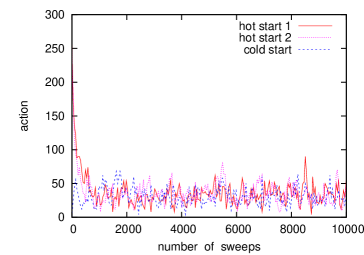
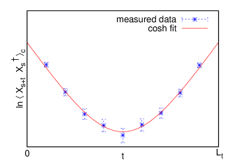
Figure 1: On the left: examples for Monte Carlo histories, i.e. the evolution of the Euclidean action $S$ depending on the number of update steps in units of “sweeps” (one update for each site of the lattice volume). We show the beginning of three histories, with two “hot starts” and one “cold start”, which soon fluctuate around the same stable plateau (at $\langle S\rangle\approx 33$). On the right: possible results for a connected correlation function, $\langle X_{s+t}X_{s}^{\dagger}\rangle_{c}$ (in $d>1$, $X_{s}$ could be a sum over a time slice, $X_{s}=\sum_{\vec{x}}X_{\vec{x},s}$, which corresponds to momentum $\vec{p}=\vec{0}$, cf. footnote 2), and a fit to the expected cosh-function of eq. (5), for periodic boundary conditions over the extent $L_{t}$ in Euclidean time. The physical interpretation of $L_{t}$ is an inverse temperature, see Appendix B.

At this point, the configurations are quite smooth. The Boltzmann factor $\exp(-S)$ favors a further decrease of $S$, but this requires specific, even smoother configurations. There are more random update suggestions which would increase $S$, but these are less likely to be accepted, due to detailed balance (7). The equilibrium between a Boltzmann effect (pulling $S$ down) and an entropy effect (pushing $S$ up) causes fluctuations around a stable mean value. This regime is independent of the initial configuration (for a cold start it is attained from below), and here the numerical measurement can be performed. The first part of the Monte Carlo history, the thermalization, is discarded — it is just needed for first taking the Markov chain to the right regime, the thermal equilibrium.

Now one still has to assure that the thermal equilibrium configurations that one uses are (essentially) independent of each other. To this end, i.e. in order to avoid auto-correlation effects, the measurements have to be separated by a sufficient number of update steps. In the example illustrated in Fig. 1 (left), one should first wait for a few thousand Monte Carlo sweeps for the thermalization. If we subsequently measure the expectation value of the action itself, $\langle S\rangle$, the separation should be a few hundred sweeps — for subtle observables it has to be longer, cf. footnote 8.

Once we have generated a sizable set of “golden configurations” (well thermalized and decorrelated), we perform the numerical measurement. Fig. 1 (right) shows, as an example, possible results for the connected correlation function of some quantity $X$ (a product of fields, often denoted as an “operator”) over different separations $t$ in Euclidean time. A fit to the expected $\cosh$ function, cf. eq. (5), yields a result for the correlation length, which represents the inverse first energy gap, $\xi=1/(E_{1}-E_{0})$. In quantum field theory, this first excitation energy above the vacuum is the mass of the (lightest) particle which corresponds to the quantity $X$.

2.4 Lattice gauge theory

Let us consider a free, complex scalar field, $\Phi_{x}\in\mathbb{C}$, with the lattice action

$$S[\Phi] = \frac{a^{d-2}}{2}\sum_{x,y}\Phi_{x}^{*}M_{xy}\Phi_{y}\ ,$$

$$M_{xy} = \sum_{\mu=1}^{d}(-\delta_{x+a\hat{\mu},y}-\delta_{x-a\hat{\mu},y}+2\delta_{x,y})+(ma)^{2}\delta_{x,y}\ ,$$ (9)

where $\hat{\mu}$ is the unit vector in $\mu$-direction. This is the most obvious lattice discretization of the continuum action $S[\Phi]=\int d^{d}x\,\Phi(x)^{*}\,[-\partial^{2}+m^{2}]\,\Phi(x)$.

We now follow the procedure, which is standard in the continuum, but we do so on the lattice. We promote the global U(1) symmetry $\Phi_{x}\to e^{{\rm i}g\varphi}\Phi_{x}$ to a local symmetry, $\varphi\to\varphi_{x}$. To this end, we replace the $\delta$-links in $M$, $\delta_{x\pm a\hat{\mu},y}$, by link variables in U(1), which transform such that gauge symmetry holds. To be explicit, we substitute in eq. (9)

$$\Phi_{x}^{*}\Phi_{x+a\hat{\mu}}\longrightarrow\Phi_{x}^{*}U_{x,\mu}\Phi_{x+a\hat{\mu}}\ ,\ \Phi_{x}^{*}\Phi_{x-a\hat{\mu}}\longrightarrow\Phi_{x}^{*}U_{x-a\hat{\mu},\mu}^{*}\Phi_{x-a\hat{\mu}}\ ,\quad U_{x,\mu}\in{\rm U}(1)\ ,$$

as illustrated in Fig. 2 (left), such that a gauge transformation

$$\Phi_{x}\to e^{{\rm i}g\varphi_{x}}\Phi_{x}\ ,\quad U_{x,\mu}\to e^{{\rm i}g\varphi_{x}}U_{x,\mu}e^{-{\rm i}g\varphi_{x+a\hat{\mu}}}$$ (10)

leaves the lattice action invariant. So we have implemented a discrete covariant derivative, which endows gauge invariance at the regularized level. Generically, such a compact link variable is an element of the gauge group (not of its algebra!), e.g. $U_{x,\mu}\in{\rm SU}(N_{c})$; then the link from $x$ in $-\mu$-direction takes the form $U_{x-a\hat{\mu},\mu}^{\dagger}$.

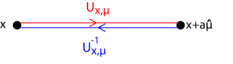
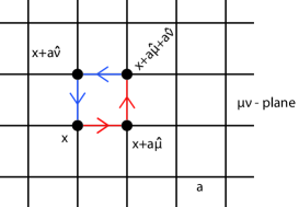
Figure 2: On the left: an compact link variable $U_{x,\mu}\in\{{\rm gauge~{}group}\}$, as part of the lattice gauge field. On the right: illustration of a plaquette variable, as given in eq. (11).

To construct the lattice gauge action, we first build the plaquette variable 

$$U_{x,\mu\nu}:=U_{x,\nu}^{-1}U_{x+a\nu,\mu}^{-1}U_{x+a\mu,\nu}U_{x,\mu}\in\{\mbox{\,gauge~{}group\,}\}\ ,$$ (11)

which represents a minimal lattice Wilson loop in the $\mu\nu$-plane, as shown in Fig. 2 (right). Therefore $U_{x,\mu\nu}$ is gauge invariant as well, and a suitable ingredient for the lattice gauge action (Wilson’s standard formulation)

$$S_{\rm gauge}[U] = \frac{2N_{c}}{g^{2}}\sum_{x,\,\mu<\nu}\Big{(}1-\frac{1}{2N_{c}}{\rm Tr}[U_{x,\mu\nu}+U_{x,\mu\nu}^{\dagger}]\Big{)}$$ (12)

$$= \frac{2N_{c}}{g^{2}}\sum_{x,\,\mu<\nu}\Big{(}1-\frac{1}{N_{c}}{\rm Re}\,{\rm Tr}\,U_{x,\mu\nu}\Big{)}\ ,\ \ {\rm for~{}}U_{x,\mu},\,U_{x,\mu\nu}\in{\rm SU}(N_{c}).\quad$$

In contrast to continuum gauge theory, no gauge fixing is needed, thanks to the use of compact link variables. This is a great relief, since it avoids nightmares related to Faddeev-Popov ghost fields. Moreover, compact link variables simplify the update procedure in the Monte Carlo simulation.

In order to confirm that the continuum limit takes the expected form, we introduce non-compact link variables $A_{x,\mu}$ (in the algebra), and the corresponding continuum field $A_{\mu}(x)$. For instance in the simple case of 4d U(1) gauge theory we obtain

$$U_{x,\mu} = \exp\Big{(}-{\rm i}g\int_{x}^{x+a\hat{\mu}}ds\,A_{\mu}(s)\Big{)}=e^{-{\rm i}gaA_{x,\mu}}\ ,\ U_{x,\mu\nu}=e^{-{\rm i}a^{2}gF_{x,\mu\nu}}\ ,$$

$$F_{x,\mu\nu} = \frac{(A_{x+a\hat{\mu},\nu}-A_{x,\nu})-(A_{x+a\hat{\nu},\mu}-A_{x,\mu})}{a}=F_{\mu\nu}(x)+{\cal O}(a)\ ,$$

$$S_{\rm gauge}[U] = \frac{1}{g^{2}}\sum_{x,\,\mu<\nu}(1-{\rm Re}\,U_{x,\mu\nu})=\frac{1}{4}\int d^{4}x\,F_{\mu\nu}(x)F_{\mu\nu}(x)+{\cal O}(a^{2})\ .$$ (13)

2.5 Fermion fields

We treat $\Psi(x)$ and $\bar{\Psi}(x)$ as independent fermion fields, and assume an action of bilinear form, with the partition function

$$Z=\int{\cal D}\bar{\Psi}\,{\cal D}\Psi\,\exp(-\bar{\Psi}M\Psi)=\int\prod_{k}d\bar{\psi}_{k}\,d\psi_{k}\,\exp\Big{(}-\sum_{ij}\bar{\psi}_{i}M_{ij}\psi_{j}\Big{)}\ .$$ (14)

The components, given by the indices $i,j,k$, run over everything, i.e. over all lattice sites, and on each site over the internal degrees of freedom, such as the spinor index and possible indices for $N_{f}$ flavors and $N_{c}$ colors.

For each spinor, the fermion matrix $M$ contains a discrete, Euclidean Dirac operator $D$. In contrast to the scalar field action in Subsection 2.4, its formulation is not straightforward, not even for free fermions. The naïve discretization of the linear derivative, $\partial_{\mu}\Psi(x)\to\frac{1}{2a}(\Psi_{x+a\hat{\mu}}-\Psi_{x-a\hat{\mu}})$, fails. It is plagued by the notorious fermion doubling problem: its free propagator in momentum space,

$$\tilde{D}_{\mbox{na\"{\i}ve}}(p)^{-1}=\Big{[}{\rm i}\gamma_{\mu}\frac{1}{a}\sin(ap_{\mu})+m\Big{]}^{-1}=\frac{-{\rm i}\gamma_{\mu}\frac{1}{a}\sin(ap_{\mu})+m}{\frac{1}{a^{2}}\sum_{\mu}\sin^{2}(ap_{\mu})+m^{2}}\ ,$$ (15)

has — in the chiral limit $m\to 0$ — $2^{d}$ poles, instead of one (in the Brillouin zone).

A number of valid formulations are known, such as the Wilson fermion:[9] $D_{\mbox{na\"{\i}ve}}$ is supplemented by a discrete Laplacian, which moves the masses of the doublers to the cutoff scale,

$$D_{\rm Wilson} = \frac{1}{2}\sum_{\mu=1}^{d}\Big{[}\gamma_{\mu}(\nabla_{\mu}+\nabla_{\mu}^{*})-a\nabla_{\mu}^{*}\nabla_{\mu}\Big{]}+m\ ,$$

$${\rm free~{}fermion:} \nabla_{\mu}\psi_{x}=(\psi_{x+a\hat{\mu}}-\psi_{x})/a\ ,\quad\nabla_{\mu}^{*}\psi_{x}=(\psi_{x}-\psi_{x-a\hat{\mu}})/a\ ,$$ (16)

where $\nabla_{\mu}$ ($\nabla_{\mu}^{*}$) is a forward (backward) lattice derivative. Unfortunately the Wilson term explicitly breaks the chiral symmetry of massless fermions, $\{D_{\rm Wilson},\gamma_{5}\}\neq 0$, which entails problems like an additive mass renormalization (see below).

The other standard formulation is known as staggered fermions:[10] a transformation replaces the $\gamma$-matrices by $x$-dependent sign factors. In $d=4$ this reduces the number of doublers by a factor of 4 (the number of spinor components), and the remaining $16/4=4$ species are used as a kind of degenerate flavors (“tastes”). Here a ${\rm U}(1)$ subgroup of the chiral symmetry persists. However, $N_{f}=4$ light quark flavors is not what we need in QCD. Formally this formulations can be generalized to one (and therefore to any) number of flavors by taking the forth root of the fermion determinant (see below), but locality is questionable for such “rooted staggered fermions”.

Since the end of the 20th century we also have formulations which preserve the full chiral flavor symmetry, ${\rm SU}(N_{f})\otimes{\rm SU}(N_{f})$, cf. Subsection 3.3, in a lattice modified form, which turns into the standard form in the continuum limit[11]. The condition for this property is the Ginsparg-Wilson Relation,[13] which reads (in its simplest form)

$$\{D,\gamma_{5}\}=aD\gamma_{5}D\ .$$ (17)

Various types of solutions are known, such as Domain Wall Fermions[14], (classically) perfect fermions[15] and overlap fermions[16], but they are all rather tedious to simulate. For reviews we refer to Refs. revGWR.

In the presence of a gauge field $U_{x,\mu}$, all these formulations of the lattice Dirac operator contain covariant lattice derivatives,

$$\nabla_{\mu}\psi_{x}=\frac{1}{a}(U_{x,\mu}\psi_{x+a\hat{\mu}}-\psi_{x})\ ,\quad\nabla_{\mu}^{*}\psi_{x}=\frac{1}{a}(\psi_{x}-U_{x-a\hat{\mu},\mu}^{-1}\psi_{x-a\hat{\mu}})\ ,$$ (18)

hence also the fermion action is gauge invariant at the regularized level. Regarding the Wilson term, $-\frac{a}{2}\nabla_{\mu}^{*}\nabla_{\mu}$, the link couplings are suppressed, whereas the on-site term $\propto\bar{\psi}_{x}\psi_{x}$ remains invariant, which leads to the aforementioned additive mass renormalization (along with further nuisance, like ${\cal O}(a)$ scaling artifacts). Hence a negative bare mass $m$ has to be tuned in order to get close to chirality; in QCD this means attaining light pions. This tuning — to search for criticality — is not needed in the cases of staggered fermions or Ginsparg-Wilson fermions, thanks to the (remnant) chiral symmetry on the lattice.

In the canonical formalism of Quantum Field Theory, Pauli’s principle — as part of the Spin-Statistics Theorem — is implemented by the anti-commutation behavior of the fermionic creation and annihilation operators. They do not occur in the functional integral formulation, so one implements the fermionic anti-commutativity by the type of fields: the components $\bar{\psi}_{i}$, $\psi_{j}$ are given by Grassmann variables, i.e. elements $\eta_{1},\eta_{2},\eta_{3}\dots$ of a Grassmann algebra, with the rules

$$\{\eta_{i},\eta_{j}\}=0\ ,\quad\frac{\partial}{\partial\eta_{i}}\eta_{j}=\delta_{ij}=\int d\eta_{i}\ \eta_{j}\ ,$$ (19)

where the integral in the last term does not have any bounds. It is defined such that it obeys translation invariance (see e.g. Ref. PS).

Application of these rules leads to the celebrated formulae

$$\int{\cal D}\bar{\Psi}\,{\cal D}\Psi\,\exp(-\bar{\Psi}M\Psi)={\rm det}\,M\ ,\quad\langle\bar{\psi}_{i}\,\psi_{j}\rangle=-(M^{-1})_{ij}\ ,$$ (20)

where ${\rm det}\,M$ is the fermion determinant. In light of these results, we see that computers do not need to handle Grassmann variables, they “just” deal with the (complex) fermion matrix $M$. However, in typical QCD simulations $\bar{\Psi}$, $\Psi$ have millions of components, hence capturing ${\rm det}\,M$ and $M^{-1}$ is a formidable task, the bottleneck in lattice QCD simulations.

In 4d lattice gauge theories, a (frequent) computation of ${\rm det}\,M$ is hardly feasible. The HMC algorithm[7] circumvents this problem as follows: first we note that all usual lattice Dirac operators $D$ are $\gamma_{5}$-Hermitian,

$$D^{\dagger}=\gamma_{5}D\gamma_{5}\quad\Rightarrow\quad H:=\gamma_{5}D=H^{\dagger}\ .$$ (21)

For two degenerate flavors, the fermion determinant is expressed by introducing an auxiliary multi-scalar field $\Phi\in\mathbb{C}^{N}$, which is denoted as a “pseudo-fermion field”,

$${\rm det}\,D[U]^{2}={\rm det}\,H[U]^{2}=\int{\cal D}\Phi^{\dagger}{\cal D}\Phi\ e^{-G^{\dagger}[U,\Phi]\,\cdot\,G[U,\Phi]}\ ,\ G[U,\Phi]:=H[U]^{-1}\Phi\ .$$ (22)

Updating the pseudo-fermion field is not necessary thanks to the Gaussian structure in $G$; this random distribution can be generated directly, as it is also done for the momentum field in the HMC algorithm; both are refreshed before beginning a new Molecular Dynamics trajectory. (There are quite efficient methods to iteratively invert a huge but sparse, positively definite matrix, like $D^{\dagger}D=H^{2}$.)

Once the fermion fields are integrated out, the configuration is given in terms of the gauge link variables, $[U]$. If we update just one link, the change of the gauge action, $\Delta S_{\rm gauge}$ in a notation analogous to eq. (7), can be computed locally, since it only affects $2(d-1)$ plaquette variables. In the presence of fermions, however, ${\rm det}\,M$ alters $S$ in a complicated manner. Now numerous degrees of freedom are coupled, and the HMC algorithm is appropriate, since it modifies the entire configuration at once. Still, the inclusion of quarks makes the generation of QCD configurations much more tedious: the computational effort increases by (about two) orders of magnitude.

3 Lattice QCD and the hadron spectrum

3.1 Set-up

As discussed in Section 2, a lattice QCD configuration $[U]$ is given by a set of link variables $U_{x,\mu}\in{\rm SU}(3)$, which connect nearest neighbor lattice sites. The gauge action (12) is obtained by summing over the plaquette variables $U_{x,\mu\nu}$, given in eq. (11). Integrating out the quark fields $\bar{\Psi}$, $\Psi$ gives rise to the fermion determinant of eq. (20). Thus the partition function takes the form

$$Z=\int{\cal D}U\ {\rm det}\,M[U]\,\exp(-S_{\rm gauge}[U])\ ,$$ (23)

i.e. the statistical weight is composed of the fermion determinant and the Boltzmann factor of the gauge action, both depending on the gauge configuration.

In lattice QCD, the prefactor of eq. (12) is usually denoted as $\beta=6/g^{2}$ (as in Statistical Mechanics). If it increases, the “golden” gauge configurations (thermalized and decorrelated) become smoother, and the physical lattice spacing $a$ decreases; $\beta\to\infty$ corresponds to the continuum limit $a\to 0$. At fixed $\beta$ one selects a phenomenologically known, dimensional quantity, which is rather easy to measure numerically, and identifies $a$ in this way[19], usually in the range $a\simeq 0.05\dots 0.1~{}{\rm fm}$. One would like $a$ to be small, to suppress the lattice artifacts, but on the other hand the physical size $La$ should be kept large enough (with the affordable number of lattice sites $L$ in one direction); it should clearly exceed the correlation length (cf. Section 2), which is given here by the inverse pion mass, $\xi=1/M_{\pi}$.

Once the Monte Carlo algorithm has generated a set of “golden” configurations with the right probability distribution, we can measure physical observables. For instance, the pseudo-scalar densities (cf. footnote 2)

$$P_{t}^{+}=\sum_{\vec{x}}\bar{d}_{\vec{x},t}\,\gamma_{5}\,u_{\vec{x},t}\ ,\quad P_{t}^{-}=\sum_{\vec{x}}\bar{u}_{\vec{x},t}\,\gamma_{5}\,d_{\vec{x},t}$$ (24)

(where $u$ and $d$ are the quark fields for the corresponding flavors) are relevant for the charged pions. $M_{{\pi}^{\pm}}$ is obtained from the decay of the correlator (at $1\ll t/a\ll L_{t}$)

$$C_{{\pi}^{\pm}}(t)=\langle\,P^{\pm}_{s+t}\,P^{\pm\,*}_{s}\,\rangle_{c}\propto\exp(-M_{\pi}^{\pm}\,t)\ ,$$ (25)

up to artifacts that we discussed in Section 2. (Of course, CPT invariance implies $M_{\pi^{+}}=M_{\pi^{-}}\,$.)

Varying the density $P_{t}^{\pm}$, both with respect to the quark flavors and the element of the Clifford algebra, leads to further hadron masses (this is nicely described in the lecture notes Marc). The same procedure allows us to measure further physical quantities, such as matrix elements, decay constants, the chiral condensate, the crossover temperature of the chiral — or confinement–deconfinement — transition, the topological susceptibility etc. These results are truly based on first principles of QCD (in contrast to many other approaches in the literature, which are QCD-related, but which ultimately depend on additional assumptions and parameters).

Of course, lattice simulations can also be applied to other models of (phenomenological or theoretical) interest, such as the Higgs sector of the Standard Model (based on triviality, an upper bound for the Higgs particle mass could be estimated, $M_{\rm Higgs}\raisebox{-2.15277pt}{$\,\stackrel{{\scriptstyle<}}{{\scriptstyle\sim}}\,$}650\,{\rm GeV}$), QED (although in that case perturbation theory is successful), and many models which are relevant e.g. in Condensed Matter Physics, Statistical Mechanics, or the search for physics beyond the Standard Model[21], including multi-flavor systems (which are fashion now, in view of a possible sub-structure of the Higgs particle[22]), Dark Matter models[23], supersymmetry (although its lattice formulation is problematic[24]), field theories in non-commutative spaces,[25] etc.

However, QCD simulations are particularly motivated, so let us focus on QCD. Fig. 3 (left) shows phenomenological data which illustrate the famous property of asymptotic freedom, i.e. the decrease of the strong gauge coupling $g_{s}$, and the corresponding quantity $\alpha_{s}$, for increasing transfer momentum $q$,

$$\alpha_{s}(q)=\frac{1}{4\pi}g_{s}(q)^{2}=\frac{6\pi}{33-2N_{f}}\,\frac{1}{\ln(q/\Lambda_{\rm QCD})}\quad\ {\rm(to~{}leading~{}order).}$$ (26)

We see that perturbation theory is applicable only at high energy, where $\alpha_{s}(q)$ becomes small, but at low energy a non-perturbative method is required.

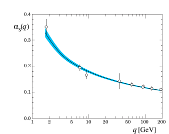
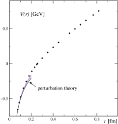
Figure 3: On the left: the strong coupling $\alpha_{s}$ of eq. (26) as a function of a transfer momentum $q$. The curve logarithmically interpolates phenomenological data points, and illustrates asymptotic freedom. On the right: the effective potential $V(r)$ for two static quarks, separated by a distance $r$. At $r\raisebox{-2.15277pt}{$\,\stackrel{{\scriptstyle>}}{{\scriptstyle\sim}}\,$}0.5\ {\rm fm}$, $V(r)$ increases linearly (plots adopted from Ref. MLlect.)

The value of $\Lambda_{\rm QCD}$ is renormalization scheme dependent, typically it is obtained in the range $200\dots 250\,{\rm MeV}$. It is remarkable that an intrinsic scale occurs; for massless quarks, the action does not involve any dimensional parameter ($g_{s}$ is dimensionless). Hence this scale is due to an anomaly: quantization explicitly breaks the scale invariance of the classical field theory. It is similar to the energy scale of the chiral condensate, which was measured in lattice simulations,

$$\Sigma=-\langle\bar{\Psi}\,\Psi\rangle\ ,\quad\Sigma^{1/3}\approx 270\ {\rm MeV}\ .$$ (27)

$\Sigma$ acts as an order parameter for chiral symmetry breaking (we refer to 2 or 3 light quark flavors at low temperature). Thus QCD sets a magnitude for the light hadron masses.

The plot in Fig. 3 (right) illustrates confinement: $V(r)$ is the energy that it takes to pull apart two static quarks by a distance $r$. At short distances it can be computed perturbatively (few gluon exchange), but the linear increase at $r\raisebox{-2.15277pt}{$\,\stackrel{{\scriptstyle>}}{{\scriptstyle\sim}}\,$}0.5\ {\rm fm}$ is measured on the lattice; up to some $r$, it agrees with experimental observations.

3.2 Hadron masses

We pointed out in Subsection 2.5 that the fermion determinant is particularly tedious to deal with; it is the bottleneck for the generation of “golden QCD configurations”. Therefore, in the last century it was ignored in many simulations; ${\rm det}\ M[U]$ was treated as a constant, only $\,\exp(-S_{\rm gauge}[U])\,$ was taken into account. This simplification is known as the quenched approximation, and there are several ways to express its meaning: in case of $N_{f}$ degenerate quark flavors, ${\rm det}\,M[U]$ contains the factor $({\rm det}\,D[U])^{N_{f}}$, where $D[U]$ is the Dirac operator for one of these flavors. In this sense, the quenched approximation corresponds to $N_{f}=0$. Alternatively, we may refer to valence quarks with an infinite mass, which also leads to ${\rm det}\,M[U]={\rm const}$. This shows that sea quarks are not included in this approximation.

So quenched simulations were using an incomplete statistical weight for the configurations. This implies a systematic error, which is hard to estimate. One could worry that it distorts the results completely, but the outcome was not that bad at all. Fig. 4 gives an overview of hadron masses, obtained quenched by the CP-PACS Collaboration[28]. Typically three input quantities are involved. We mentioned before that measuring one phenomenologically known, dimensional quantity sets an overall scale. The bare light quark masses are assumed to be degenerate, $m_{u}=m_{d}$, and tuned for a suitable value of $M_{\pi}$, and some strange hadron mass fixes the bare quark mass $m_{s}$. This set of hadrons does not include heavier valence quarks ($c$, $b$, $t$), and their sea quark contribution is negligible at low energy (up to a minor shift in the short-distance coupling).

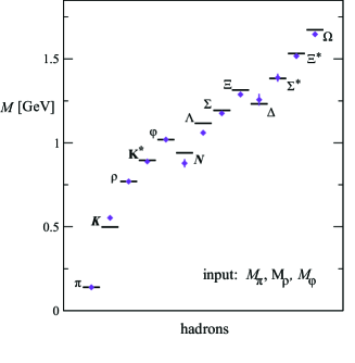
Figure 4: The light hadron spectrum obtained by the CP-PACS Collaboration[28] from lattice QCD in the quenched approximation. The masses agree with the phenomenological values (horizontal bars) up to ${\cal O}(10)\,\%$ (plot adopted from Ref. MLlect, in a modified form).

For the results of Fig. 4, these three input terms are the masses $M_{\pi}$, $M_{\rho}$ and $M_{\phi}$, and all the rest are lattice predictions. We see that the agreement with the phenomenological values (horizontal bars) is quite good, it matches up to ${\cal O}(10)\,\%$. This is even more impressive when we consider that — for technical reasons — quenched QCD simulations were often performed at heavy pion masses, like $M_{\pi}\raisebox{-2.15277pt}{$\,\stackrel{{\scriptstyle>}}{{\scriptstyle\sim}}\,$}600\,{\rm MeV}$, followed by a quasi-chiral extrapolation to the physical value $M_{\pi}\approx 138\,{\rm MeV}$, which caused additional uncertainties.

Hence quenched simulation results already indicated that QCD is promising to work also at low energy. Of course, the lattice community wanted to proceed to precise large-scale simulations with dynamical quarks. This was achieved in the 21st century, with rapid progress based on improvements in many respects (computers, algorithms, lattice actions, numerical measurement techniques etc.).

Fig. 5 shows results by the Budapest-Marseille-Wuppertal Collaboration[30]. If we assume an exponential decay of a hadronic correlation function $C$, as in the example of eq. (25), we can extract the corresponding hadron mass $M$ as

$$M=\frac{1}{a}\ln\Big{(}\frac{C_{t}}{C_{t+a}}\Big{)}\ .$$ (28)

In practice the results depend on the distance $t$. The exponential that we refer to is actually just the leading contribution to a superposition of exponentials, which includes excited states, so at short $t$ contaminations by higher states are expected. As $t$ grows, they are exponentially suppressed and the first energy gap dominates, which suggests to take $t$ as large as possible. One should not overdo it, however, because at large $t$ the wanted signal is exponentially suppressed too (though in a weaker form), and it eventually disappears in the statistical noise. Hence one hopes to find a suitable interval of moderate $t$, where $M$ is stable and conclusive. Such intervals can be observed in the first plot of Fig. 5 (left), for five hadron masses.

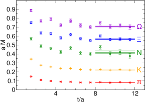
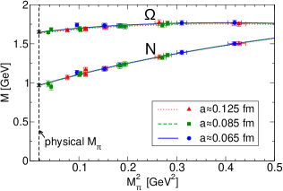
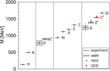
Figure 5: The hadron spectrum, obtained by the Budapest-Marseille-Wuppertal Collaboration by QCD simulations with $2+1$ flavors of dynamical quarks.[30] On the left: illustration of the mass plateaux, which provide reliable values for a set of hadron masses, cf. eq. (28). On the right: extrapolation of two baryon masses to the physical point, where $M_{\pi}$ takes its phenomenological value. Below: overview over the extrapolated hadron spectrum, compared to the experimental results (plots adopted from Ref. BMW).

A set of pion masses was simulated, which reached down to $M_{\pi}\approx 190\,{\rm MeV}$, i.e. quite close to the physical value. Fig. 5 (right) shows how two baryon masses depend on $M_{\pi}^{2}$, and how they are extrapolated to the physical pion mass, which is also here an input parameter.

The system size was kept at $La\simeq 4/M_{\pi}$, so it attained $\approx 4\,{\rm fm}$, which suppresses finite size effects quite well. Regarding the lattice artifacts, three different lattice spacings were used as a basis for the continuum extrapolation, $a=0.125\,{\rm fm},\ 0.085\,{\rm fm},\ 0.065\,{\rm fm}$. In this way, the spectrum in Fig. 5 (bottom) was obtained, in excellent agreement with phenomenology. Referring to Section 1, we are most interested in the nucleon mass, which was measured as

$$M_{\rm N}=936(25)(22)\,{\rm MeV}\ ,$$ (29)

in accurate agreement with Nature. The parentheses give the statistical and systematic errors, respectively, which sum up to $3.6\,\%$.

A new strategy was introduced in Ref. QCDSFPLB. The traditional approach for 2+1 flavors ($m_{u}=m_{d}\ll m_{s}$) proceeded as follows:

• Adjust the kaon mass, $M_{K}\simeq 496\,{\rm MeV}$, as well as possible.

• Now push for light pions, while keeping $M_{K}\approx{\rm const.}$

The new approach by the QCDSF-UKQCD Collaboration proceeds in a different manner, which is illustrated in Fig. 6.

• Start from SU(3)_f flavor symmetry, i.e. $m_{u}=m_{d}=m_{s}$ and $M_{\pi}=M_{K}$. In this setting, the “center of squared masses” of the pseudoscalar meson octet,

  $$X_{\pi}^{2}:=\frac{1}{3}(M_{\pi}^{2}+2M_{K}^{2})\ ,$$ (30)

  is tuned to its physical value.

• Now decrease the light quark mass $m_{q}:=m_{u}=m_{d}$ while increasing $m_{s}$. This simultaneous modification is performed such that $X_{\pi}$ is kept constant, while $M_{\pi}$ and $M_{K}$ extrapolate to their physical values.

  This trajectory towards the physical point is constrained and stable. It is located inside the regime where Chiral Perturbation Theory applies, which guides the extrapolation. Flavor singlet quantities, like $X_{\pi}$, change only in the second order of the variation of the renormalized quark masses.

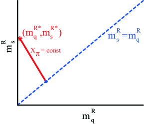
Figure 6: Scheme of the renormalized quark masses $m_{q}^{R}:=m_{u}^{R}=m_{d}^{R}$ and $m_{s}^{R}$.[31] SU(3)_f flavor symmetry is realized on the dashed line, where we select the point with the physical value of $X_{\pi}$. From there we decrease $m_{q}^{R}$, and increase $m_{s}^{R}$, such that $X_{\pi}$ is preserved, and we approach the physical masses $M_{\pi}$ and $M_{K}$. This is the point to determine a multitude of further hadron masses.

The application of this method[32] led to the hadron spectrum in Fig. 7. It was obtained in the lattice volumes $V=24^{3}\times 48$ and $32^{3}\times 64$, at a lattice spacing $a=0.0765(15)~{}{\rm fm}$. We see an accurate agreement with the phenomenological masses, up to the baryon $\Omega\sim(sss)$.

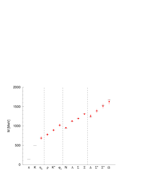
Figure 7: The hadron spectrum obtained by the QCDSF-UKQCD Collaboration[32] from QCD simulations with $2+1$ flavors of dynamical quark. $M_{\pi}$ and $M_{K}$ are input quantities, and all the rest agrees with phenomenology within small errors (plot from Ref. QCDSFPRD, in modified form).

Further collaborations have arrived at similar results. In light of these data, no doubt remains that QCD is the appropriate theory for hadron physics down to low energy. Overviews of the lattice results on light hadrons are given in Refs. FodHoel and FLAG; the latter contains carefully evaluated “world averages” for hadron masses, and numerous additional quantities like quark masses, Low Energy Constants, decay constants, meson mixing parameters, form factors and the running coupling $\alpha_{s}$. We also refer to the review talks at the annual Lattice Symposium; since 2005 the proceedings appear in Proc. of Science (PoS).

3.3 Lattice QCD and chiral perturbation theory

Before the breakthrough of lattice QCD, low energy QCD was most successfully described by the effective Lagrangian of Chiral Perturbation Theory. Unlike ad hoc effective models, it is manifestly derived from QCD with light quark flavors. In the limit of massless quarks, the left- and right-handed quark field decouple,

$${\cal L}^{\rm QCD}_{m_{\rm quark}=0}=\bar{\Psi}_{L}D\Psi_{L}+\bar{\Psi}_{R}D\Psi_{R}+{\cal L}_{\rm gauge}\ ,$$ (31)

where $\bar{\Psi}$, $\Psi$ run over $N_{f}$ flavors, and $D$ is the (joint) Dirac operator. Thus ${\cal L}^{\rm QCD}_{m_{\rm quark}=0}$ has a global $U(N_{f})_{L}\otimes U(N_{f})_{R}$ symmetry, which can be decomposed into subgroups,

$${\rm U}(N_{f})_{L}\otimes{\rm U}(N_{f})_{R}={\underbrace{{\rm SU}(N_{f})_{L}\otimes{\rm SU}(N_{f})_{R}}_{\rm chiral~{}flavor~{}symmetry}}\otimes{\underbrace{{\rm U}(1)_{L=R}}_{\rm baryon~{}number}}\otimes{\underbrace{{\rm U}(1)_{\rm axial}}_{\rm anomalous}}\ .$$ (32)

One U(1) symmetry breaks explicitly under quantization (axial anomaly). The other one is chirality-blind and responsible for baryon number conversation. We are interested in the remaining chiral flavor symmetry, which breaks spontaneously,

$${\rm SU}(N_{f})_{L}\otimes{\rm SU}(N_{f})_{R}\to{\rm SU}(N_{f})_{L=R}\ .$$ (33)

This yields $N_{f}^{2}-1$ Nambu-Goldstone Bosons (NGBs), or light quasi-NGBs if we include small quark masses. They dominate the low energy physics, and Chiral Perturbation Theory deals with a Lagrangian for these quasi-NGBs, which are identified with the light mesons (pions for $N_{f}=2$; $\pi,\,K,\,\eta$ for $N_{f}=3$).

Hence Chiral Perturbation Theory deals with fields in the coset space of the spontaneous symmetry breaking, $U(x)\in{\rm SU}(N_{f})$.[35] It includes all terms, which obey the chiral flavor symmetry (as well as Lorentz invariance and locality). They are structured in a hierarchical order, according to the energy (powers of momenta, and of quark or meson masses).

Here we consider $N_{f}=2$, such that the field $U(x)\in{\rm SU}(2)$ describes the pion triplet $\pi^{+},\,\pi^{0},\,\pi^{-}$, and we assume a (degenerate) mass $m_{q}$ for $u$ and $d$ quarks. The leading and some sub-leading terms of the effective Lagrangian can be written as

$${\cal L}_{\rm eff}(U,\partial_{\mu}U)=\frac{F_{\pi}^{2}}{4}\,{\rm Tr}[\partial_{\mu}U^{\dagger}\partial_{\mu}U]+\frac{\Sigma\,m_{q}}{2}\,{\rm Tr}[U^{\dagger}+U]$$

$$+\,l_{1}\ ({\rm Tr}[\partial_{\mu}U^{\dagger}\partial_{\mu}U])^{2}+l_{2}\ ({\rm Tr}[\partial_{\mu}U^{\dagger}\partial_{\nu}U])^{2}+l_{3}\ \Big{(}\frac{\Sigma m_{q}}{F_{\pi}^{2}}\Big{)}^{2}({\rm Tr}[U^{\dagger}+U])^{2}+\dots$$ (34)

The coefficients to these terms are known as Low Energy Constants (LECs); they appear in the effective theory as free parameters. Hence ${\cal L}_{\rm eff}$ is derived from QCD, but — being a simplification — it cannot capture its entire information.

The leading order LECs are the pion decay constant $F_{\pi}$ and the chiral condensate $\Sigma$, while the $l_{i}$ appear in sub-leading terms. The LECs of the effective theory can only be determined from the underlying, fundamental theory, which is QCD in this case. Since this refers to low energy, it is a non-perturbative problem, and therefore a challenge for lattice simulations. If this works, we arrive at a rather comprehensive picture of low energy QCD.

Chiral Perturbation Theory has been formulated and studied in various regimes, depending on the volume:

• $p$-regime[36]: the volume is large, e.g. $V=L^{4}$, $L\gg M_{\pi}^{-1}$, and the momentum of $U(x)$ counts (in the energy hierarchy) like $M_{\pi}$.

• $\epsilon$-regime[37]: the volume is small, $L\raisebox{-2.15277pt}{$\,\stackrel{{\scriptstyle<}}{{\scriptstyle\sim}}\,$}M_{\pi}^{-1}$, and a momentum counts like $m_{q}$.

• $\delta$-regime[38]: the spatial volume is small, but the extent in Euclidean time is large, e.g. $V=L^{3}\times L_{t}$, $L\raisebox{-2.15277pt}{$\,\stackrel{{\scriptstyle<}}{{\scriptstyle\sim}}\,$}M_{\pi}^{-1}\ll L_{t}$.

The $p$-regime is standard, and also the $\epsilon$-regime has been studied extensively, both analytically[39] and numerically. The LECs are the same in all three regimes, hence the $\epsilon$-regime is convenient for their determination by simulations, which do not require large volumes. Since chirality is vital in this context, it is appropriate to use Ginsparg-Wilson fermions for the quarks. This is computationally expensive, so it was done in the quenched approximation even in this century, which led to decent results for the leading LECs. For instance, Random Matrix Theory predictions[40] for the low lying Dirac eigenvalues match the numerical data well, and the fit determines $\Sigma$.[41, 42] $F_{\pi}$ is easier to extract from the correlation of axial currents,[43, 42] or of pseudo-scalar zero modes.[44, 42] Recent progress, now with dynamical quark simulations, is reviewed in Ref. Giusti.

Here we discuss the least explored case, the $\delta$-regime (for a recent study, see Ref. Tibur). The corresponding volume is illustrated in Fig. 8 (left). Its quasi-1d form enables an approximate analytical treatment as a quantum mechanical system, i.e. a 1d O(4) model[38] (due to the local isomorphy ${\rm O}(4)\sim{\rm SU}(2)\otimes{\rm SU}(2)$).

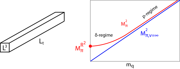
Figure 8: A schematic illustration of a volume, which corresponds to the $\delta$-regime (left) and of the quark mass dependence of $M_{\pi}^{2}$: at large $m_{q}$ it approaches $M_{\pi}^{2}\propto m_{q}$, whereas the chiral limit leads to the residual pion mass $M_{\pi}^{R}$.

Since the spatial volume is finite, there is no spontaneous symmetry breaking, and pions do not become massless NGBs at $m_{q}\to 0$. Instead they keep a residual mass $M_{\pi}^{R}$ in the chiral limit. On the other hand, at large $m_{q}$ the same volume appears large, and we obtain the $p$-regime behavior, namely the Gell-Mann–Oakes–Renner Relation $M_{\pi}^{2}\approx(\Sigma/F_{\pi}^{2})\,m_{q}$. This is shown schematically in Fig. 8 (right).

We return to the picture of an O(4) rotor: the first gap in its energy spectrum $E_{n}=n(n+2)/(2\Theta)$ ($n=0,1,2\dots$) determines the residual pion mass, $M_{\pi}^{R}=3/(2\Theta)$. The question is how to identify $\Theta$, the moment of inertia. An expansion in inverse powers of $(F_{\pi}L)^{2}$ yields

$$LM_{\pi}^{R}=\frac{3}{2(F_{\pi}L)^{2}(1+\Delta)}\ ,\quad\Delta=\frac{0.452\dots}{(F_{\pi}L)^{2}}+{\cal O}\Big{(}\frac{1}{(F_{\pi}L)^{4}}\Big{)}\ .$$ (35)

The first order ($\Delta=0$) was derived in Ref. deltareg, and the second order in Ref. HasNie. For the third order Refs. Has10,NieWei obtained slightly different results, but for sure at this level some sub-leading LECs $l_{i}$ enter.

The QCDSF Collaboration performed extrapolations of numerical pion mass measurements into the $\delta$-regime[50], and obtained good agreement with these predictions, see Fig. 9.

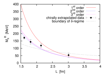
Figure 9: The residual pion mass in the $\delta$-regime of QCD. We show the predictions of the first[38], second[47] and third[48] order $\delta$-expansion; the latter two are close, which indicates convergence. The data points are extrapolated numerical results by the QCDSF Collaboration[50], which agree well with the quasi-converged $\delta$-expansion (plot from the second article cited in Ref. QCDSFdelta).

In the sub-leading order of the effective Lagrangian, the least known — and most controversial LEC — is $l_{3}$. Its value is usually taken at the energy of the physical pion mass, where it is denoted as $\bar{l}_{3}$. If we fix the other LECs involved to their known values, the QCDSF numerical results suggest $\bar{l}_{3}=4.2(2)$, somewhat above the world-average according to the FLAG report[34],  $\bar{l}_{3}|_{N_{f}=2}=3.41(41)$.

4 Status and challenges of the future

Regarding the light hadron spectrum, low energy QCD is now systematically tested from first principles: lattice simulations consistently confirm the phenomenological values up to ${\cal O}(1)\,\%$ uncertainty. This was a key point in the ambitious program, which was outlined in the 1980s. In particular, the precise results for the nucleon mass explain over $99\,\%$ of the mass of known matter in the visible Universe.

Of course, lattice QCD results involve many quantities, beyond hadron masses and Low Energy Constants, which were not discussed here: decay constants, matrix elements, quark masses and the strong coupling $\alpha_{s}$, flavor mixing parameters, thermodynamic properties, ingredients of structure functions, spin and (anomalous) magnetic momenta, quark and gluon propagators, vertex functions, etc. Here we sketched the basic ideas — they are explained in detail in six text books[1] devoted to this subject — and we showed a few selected examples; for a comprehensive overview of results (with light quarks) we refer again to Ref. FLAG.

We mentioned before that — in the early period — Kenneth Wilson was the main protagonist of the lattice approach to QCD. At the end of the 1980s, however, he suddenly expressed his pessimism about its prospects in any foreseeable future, and he left the field. However, the lattice community kept working and growing: the annual Lattice Symposium started as a small event in the 1980s, and attracted already some 300 participants in the 1990s. Nowadays the number is around 500, and the total community is certainly more than twice that large. Unfortunately, Latin America is still drastically under-represented, we hope for that to change in the future. Actually it is becoming easier to contribute even without huge computational resources, thanks to the International Lattice Data Grid,[51] which makes valuable QCD configurations publically available.

Regarding Wilson’s pessimism, we add that indeed it took time to arrive at percent level results for phenomenological quantities, but this has now been achieved.

So what is next? Meanwhile the lattice community is already pushing for the sub-percent level. This is not a straightforward extension, but it requires qualitatively new aspects: for instance QED effects and the splitting between the masses $m_{u}$ and $m_{d}$ have to be considered at that level of precision. As a remarkable result, even the splitting between the neutron and proton mass has been demonstrated[52]: it was shown that QCD implies in fact $M_{\rm neutron}>M_{\rm proton}$ — a property, which is highly non-trivial, with far-reaching consequences like the proton stability. Moreover the scenario with a quark mass $m_{u}=0$ — which would have solved the strong CP problem — could be safely ruled out.[34, 53]

Nevertheless there are still many outstanding challenges.[21] For instance, the masses of excited states are far more difficult to extract, hence their uncertainties are much larger. A notorious example is the Roper resonance, $N^{*}(1440)$, where most lattice studies arrived at energies well above the phenomenological value (compared to the negative parity state $N^{*}(1535)$, the masses are often obtained in inverse order). The current status and recent progress are discussed in Ref. Leinw.

A general goal for the future is the step from post-dictions (reproduction of experimentally known facts from QCD) to predictions. Indeed, an example was given already, in the framework of heavy quarks. They are difficult to handle on the lattice, due to the short Compton wavelength. Nevertheless, in 2005 Ref. HPQCD predicted the mass of the $B_{c}^{\pm}$ meson as $6.30(2)\,{\rm GeV}$, and one year later it was indeed measured experimentally[56] at $6.286(5)\,{\rm GeV}$ (meanwhile the value slipped slightly down to $6.275(1)\,{\rm GeV}$).[57]

So is everything going to continue smoothly, with straightforward progress and constant success? This would by untypical for the history of science, and in fact there are still severe conceptual obstacles ahead of us, which cannot be overcome just by computer power. In the appendices we comment on two examples.

Appendix A Numerical measurements at fixed topology

In some field theory models, including QCD, the configurations occur in distinct topological sectors, labelled by a topological charge $Q\in\mathbb{Z}$. In the continuum, configurations can only be deformed continuously within the same sector (with periodic boundary conditions, at finite action).

Strictly speaking, there are no topological sectors on the lattice (in most formulations). Nevertheless there are ways to define a topological charge $Q$ for the lattice configurations. Continuous transitions are possible, but they have to pass through a region of high Euclidean action, which is statistically suppressed. As we make the lattice spacing finer and finer, we approach more and more the continuum behavior of infinite potential barriers. This means that an algorithm, which performs small update steps, tends to be blocked in one sector for a very long (computation) time, i.e. the auto-correlation time with respect to $Q$ gets very long.[58]

This could in principle be overcome by an algorithm, which performs large leaps to generate its Markov chain, like a cluster algorithm, but for lattice QCD no efficient algorithm of this kind is known. So far, there is no actual competitor of the HMC algorithm, which proceeds in small update steps (regarding the Molecular Dynamics evolution). Hence the problem of “topological freezing” is expected to become severe when we proceed to finer lattices. Up to now, most simulations were performed at $0.05\,{\rm fm}\raisebox{-2.15277pt}{$\,\stackrel{{\scriptstyle<}}{{\scriptstyle\sim}}\,$}a\raisebox{-2.15277pt}{$\,\stackrel{{\scriptstyle<}}{{\scriptstyle\sim}}\,$}0.1\,{\rm fm}$. When we try to further suppress this source of systematic errors and work at $a\raisebox{-2.15277pt}{$\,\stackrel{{\scriptstyle<}}{{\scriptstyle\sim}}\,$}0.05\,{\rm fm}$, the energy barriers between the topological sectors increase and tunnelling between them will be extremely rare.

This also depends on the (lightest) quark masses involved, cf. footnote 18. For instance, in the quenched approximation, at moderate lattice spacing, tunnelling happens quite easily, and one can measure e.g. the topological susceptibility

$$\chi_{\rm t}=\frac{1}{V}\Big{(}\langle Q^{2}\rangle-\langle Q\rangle^{2}\Big{)}$$ (36)

directly, or by a Gaussian interpolation of a topological charge histogram. (In QCD parity symmetry holds, hence the second term vanishes, $\langle Q\rangle=0$.) Examples for quenched QCD results,[42] with $Q$ defined by the index of the standard overlap Dirac operator[16], or an improved version, the overlap-hypercube Dirac operator[59], are shown in Fig. 10.

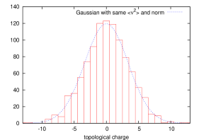
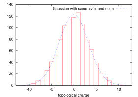
Figure 10: Histograms for topological charges of lattice QCD configurations[42], defined by the index of two variants of a chiral lattice Dirac operator, (standard) overlap[16] and (improved) hypercube-overlap[59]. These histograms are compatible with a Gauss distribution, and its width determines the topological susceptibility $\chi_{\rm t}$ (plots adopted from Ref. Stani).

They are compatible with a Gaussian distribution. Its width corresponds to a value of $\chi_{\rm t}$, which (roughly) supports the Witten-Veneziano formula[60]. This formula relates the mass of the $\eta^{\prime}$-meson to the quenched value of $\chi_{\rm t}$, based on a $1/N_{c}$ expansion. Its simplest form reads

$$M_{\eta^{\prime}}^{2}\approx\frac{2N_{f}}{F_{\pi}^{2}}\chi_{\rm t}\qquad(M_{\eta^{\prime}}\simeq 957.8\,{\rm MeV},\ F_{\pi}\simeq 92.2\,{\rm MeV})\ .$$ (37)

This formula explains the amazingly heavy $M_{\eta^{\prime}}$ (“U(1) problem”) quantitatively, as a topological effect.

In view of this straight way to determine $\chi_{\rm t}$, it seems questionable if this quantity can be measured based on data of a Monte Carlo history, which never — or hardly ever — changes the topological sector. However, several methods for this purpose were proposed, and recently also tested, and it turns out to be possible under suitable conditions. In particular, the Aoki-Fukaya-Hashimoto-Onogi formula[61]

$$^{\lim}_{|x|\to\infty}\ \langle q_{0}\,q_{x}\rangle_{|Q|}\simeq-\frac{\chi_{\rm t}}{V}+\frac{Q^{2}}{V^{2}}+\dots$$ (38)

allows for an (approximate) determination of $\chi_{\rm t}$ based on the correlation of the topological charge density $q_{x}$, measured at fixed $|Q|$. Successful tests of this approach, and variants, are reported in Refs. AFHOresults,Arthur16.

An alternative approach divides the volume into sub-volumes (“slabs”) and determines $\chi_{\rm t}$ from the topological charge distributions in these slabs. There the density is summed up, $q=\sum_{x\in{\rm slab}}q_{x}$ ($q$ does not need to be integer, since not all slab boundaries are periodic). Assuming the probability distribution $p(q)$ to be Gaussian, we obtain for two slabs — with volumes $xV$ and $(1-x)V$ — in the sector with total topological charge $Q$,

$$p_{1}(q)\cdot p_{2}(Q-q)|_{Q} \propto \exp\Big{(}-\frac{q^{2}}{2\chi_{\rm t}xV}\Big{)}\ \exp\Big{(}-\frac{(Q-q)^{2}}{2\chi_{\rm t}(1-x)V}\Big{)}$$ (39)

$$\propto \exp\Big{(}-\frac{1}{2\chi_{\rm t}V}\frac{(q-xQ)^{2}}{x(1-x)}\Big{)}\ .$$

Numerical data for $\langle(q-xQ)^{2}\rangle$, as a function of $x\in(0,1)$, in a fixed sector $Q$, enable therefore the determination of $\chi_{\rm t}$, which was confirmed in tests with non-linear $\sigma$-models[64] and 2-flavor QCD[63]. For a related approach, see Ref. LSD.

Another method, which is specific to the simulation with dynamical overlap quarks, was suggested in Ref. Egri. This is the setting where the most extreme topological freezing has been observed[67].

More generally, the question is how to measure any observable, if the Monte Carlo histories are trapped in one topological sector. Ref. Liao suggests to gradually fill the potential valleys inside the topological sectors, such that transitions occur. Thus one simulates with modified Boltzmann probabilities, to be corrected at the end by reweighting.

Alternatively, it has been advocated to prevent “topological freezing” by the use of partially open boundary conditions[69]. Since this breaks lattice translation invariance, also a milder form was proposed (a parity flip at the boundary)[70]. In these scenarios, $Q$ is not integer anymore, so it can change continuously.

However, it would be nicer to maintain periodic boundaries, and therefore $Q\in\mathbb{Z}$. Indeed, there is hope for an (approximate) determination of an expectation value of some observable, $\langle\Omega\rangle$, even if only topologically restricted measurements, i.e. results for $\langle\Omega\rangle_{|Q|}$, are available. Brower, Chandrasekharan, Negele and Wiese derived the approximation[71]

$$\langle\Omega\rangle_{|Q|}\approx\langle\Omega\rangle+\frac{c}{V\chi_{\rm t}}\Big{(}1-\frac{Q^{2}}{V\chi_{\rm t}}\Big{)}\ ,\quad(c={\rm const.})\ .$$ (40)

In an extremely large volume $V$, any sector provides the same — correct – result. However, in moderate volumes, where simulations are more realistic, a set of results for the left-hand-side, in various $V$ and $|Q|$, and a 3-parameter fit allow for the determination of the unknown terms $\langle\Omega\rangle$, $\chi_{\rm t}$ and $c$, where the former two are of physical interest. These three terms are $V$-independent, up to ordinary finite size effects, which tend to be exponentially suppressed (cf. Section 2). In contrast, the topologically restricted quantities suffer from polynomial finite size effects, as eqs. (38) and (40) show.

The latter is the beginning of an expansion in $1/(V\chi_{\rm t})$, which has recently been extended,[72] and even ordinary finite size effects have been included[73]. Detailed tests[74] in four models confirm that this method can provide accurate results for $\langle\Omega\rangle$ under suitable conditions: $V\chi_{\rm t}=\langle Q^{2}\rangle>1$ and sectors with small $|Q|$ ($|Q|\leq 1$, or perhaps $|Q|\leq 2$). For the determination of $\chi_{\rm t}$, however, the approaches of Refs. AFHO,AFHOresults,slab provide better results.

Appendix B Quantum simulations as a remedy to the sign problem?

Let us finally address the phase diagram of QCD. Finite temperature QCD is difficult to explore, since the Euclidean time direction has to be much shorter than the spatial direction, say $V=L^{3}\times L_{t}$, $L_{t}\ll L$. Let’s consider lattice units: if the computational resources set a limit like $L=32$, for example, then $L_{t}$ must be really short (in the past it was often just $L_{t}=4$). Converting it into a temperature of interest (now in physical units, with $k_{B}=1$), $T=1/(aL_{t})$, requires a large physical lattice spacing $a$, which leads to bad lattice artifacts.

Hence the finite temperature behavior has been a challenge for a long time, and the results were controversial. However, over the last decade also this issue has been settled quite well, thanks to improved simulations.[75] A confinement–deconfinement crossover was observed, which seems to coincide with the chiral symmetry breaking/restoration transition (we mentioned the chiral condensate $\Sigma$ of eq. (27) as the order parameter). It would be a phase transition for massless quarks, but since it is only a crossover, the exact transition temperature is somewhat criterion dependent; at $N_{f}=3$, values were obtained in the range[76]

$$T_{\rm crossover}\simeq 150\dots 160\,{\rm MeV}\ .$$ (41)

(In this case, the quenched approximation deviates strongly, $T_{\rm crossover}^{\rm quenched}\simeq 270\,{\rm MeV}$.)

However, the question what happens at high baryon density is even more difficult to explore, and still open. There are data from laboratories like the LHC (at CERN) and RHIC (at BNL), and observations from extremely dense objects, in particular neutron stars, as well as numerous theoretical conjectures. Still, the QCD phase diagram at high density is one of the major mysteries within the Standard Model that still persists. Fig. 11 (left) shows a cartoon of the unknown phase diagram. A large chemical potential $\mu_{B}$ corresponds to high baryon density, which occurs under exotic circumstances (the nucleon mass can be taken as a reference scale).

The reason why — unlike other issues — this hasn’t been settled yet by lattice simulations is the sign problem: the inclusion of $\mu_{B}$ attaches an imaginary part to the Euclidean action $S_{\rm QCD}$.[77] Thus one faces the problem mentioned in footnote 3; the quantity of eq. (3) becomes complex,

$$p[U]=\left.\frac{1}{Z}\exp(-S_{\rm QCD}[U])\right|_{\mu_{B}>0}\notin{\kern 2.5pt\sf{R}\kern-7.79999pt\sf{I}\kern 7.79999pt\kern-2.5pt}\ .$$ (42)

Obviously, in this setting $p[U]$ does not define any probability, and the straightforward approach to simulate QCD as a statistical system fails.

One could still perform simulations, say with $|\exp(-S_{\rm QCD})|$ and incorporate the complex phase a posteriori by reweighting. This is correct in principal, but in practice it leads to lots of cancellations, and the wanted signal is hard to extract: for stable statistical errors, the required amount of data grows exponentially in the volume. This is the technical meaning of the notorious “sign problem”, which usually prevents us from arriving at conclusive results (except at small $\mu_{B}$).

Many attempts have been – and are being — made to overcome this problem (Taylor expansion in $\mu_{B}/T$, extrapolation from imaginary $\mu_{B}$, world line formalism, complex Langevin algorithm etc.)[77], but there is no real breakthrough so far. An approach, which bears the potential of a solution, is the application of quantum (rather than classical) computing, where the complex phase is naturally incorporated. Digital quantum computers are still very far from being powerful enough for such tasks, but there is rapid progress in analog quantum computing, for instance employing ultracold atoms (at nK temperatures) trapped in optical lattices.[78] Such lattices are built by the nodes of standing laser waves, see Fig. 11 (center/right).

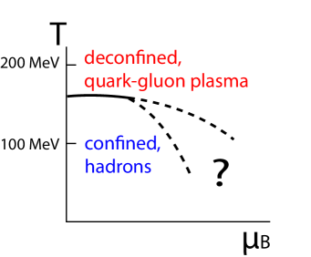
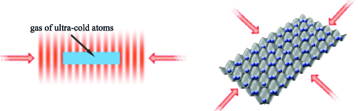
Figure 11: On the left: cartoon of the QCD phase diagram, where an increasing chemical potential $\mu_{B}$ corresponds to higher baryon density. At low density the crossover temperature is known, but the phase structure at high density is still terra incognita. Center and right: illustrations of an optical lattice, built from standing waves of laser light. Ultracold atoms may be trapped on the sites and thus physically implement a lattice field theory.

The corresponding literature is tremendous; for lack of space and knowledge, we only mention one recent proposal to quantum simulate the 2d CP(2) model (or higher CP$(N-1)$ models).[79] This toy model shares a number of qualitative features with QCD: asymptotic freedom, a dynamically generated mass gap, topological sectors, a unitary global symmetry (which may break spontaneously) and even a local symmetry.[80]

The proposed scenario uses ultracold alkaline earth atoms located on the sites of a rectangular optical $L\times L^{\prime}$ lattice, with $L\gg L^{\prime}$ (Fig. 11, center/right). The relevant degrees of freedom are the nuclear spins, which represent an SU(3) field (a staggered atomic site occupation yields anti-ferromagnetic coupling). When the (2+1)-d system approaches its continuum limit (where the correlation length diverges), it undergoes dimensional reduction (the $L^{\prime}$-direction becomes negligible), as well as spontaneous symmetry breaking SU(3) $\to$ U(2). The low energy effective theory for the four NGBs (cf. Subsection 3.3) just matches the 2d CP(2) model.

The experimental realization is feasible by means of established techniques.[79] It would allow for the measurement of quantities like the phase diagram at high density and real-time dynamics, which are unaccessible to simulations on classical computers, because of the sign problem. This would mean a step forward towards the long-term goal of a quantum simulation of high density QCD, which could explore the unknown main part, the terra incognita, of the QCD phase diagram.

References

- [1] M. Creutz, Quarks, Gluons and Lattices (Cambridge University Press, 1983). H.J. Rothe, Lattice Gauge Theories: An Introduction (World Scientific, 1992) I. Montvay and G. Münster, Quantum Fields on a Lattice (Cambridge University Press, 1994). J. Smit, Introduction to Quantum Fields on a Lattice (Cambridge University Press, 2002). T. DeGrand and C. DeTar, Lattice Methods for Quantum Chromodynamics (World Scientific, 2006). C. Gattringer and C.B. Lang, Quantum Chromodynamics on the Lattice (Springer, 2009).
- [2] K.G. Wilson and J.B. Kogut, Phys. Rept. 12 (1974) 75.
- [3] W.H. Press, S.A. Teukolsky, W.T. Vetterling and B.P. Flannery, Numerical Recipes, The Art of Scientific Computing (Cambridge University Press, 2007 (3rd edition)).
- [4] M. Creutz and B. Freedman, Ann. Phys. (N.Y.) 132 (1981) 427.
- [5] R.H. Swendsen and J.-S. Wang, Phys. Rev. Lett. 58 (1987) 86. U. Wolff, Phys. Rev. Lett. 62 (1989) 361.
- [6] S. Chandrasekharan and U.-J. Wiese, Phys. Rev. Lett. 83 (1999) 3116.
- [7] S. Duane, A.D. Kennedy, B.J. Pendleton and D. Roweth, Phys. Lett. B 195 (1987) 216.
- [8] G. Parisi and Y.-S. Wu, Sci. Sin. 24 (1981) 483.
- [9] K.G. Wilson, in New Phenomena in Subnuclear Physics, ed. A. Zichichi (Plenum, 1979), p. 69.
- [10] J.B. Kogut and L. Susskind, Phys. Rev. D 11 (1975) 395.
- [11] M. Lüscher, Phys. Lett. B 428 (1998) 342.
- [12] M. Lüscher, Nucl. Phys. B 549 (1999) 295.
- [13] P.H. Ginsparg and K.G. Wilson, Phys. Rev. D 25 (1982) 2649.
- [14] D.B. Kaplan, Phys. Lett. B 288 (1992) 342.
- [15] U.-J. Wiese, Phys. Lett. B 315 (1993) 417. W. Bietenholz and U.-J. Wiese, Nucl. Phys. B (Proc. Suppl.) 34 (1994) 516; Phys. Lett. B 378 (1996) 222; Nucl. Phys. B 464 (1996) 319. P. Hasenfratz, V. Laliena and F. Niedermayer, Phys. Lett. B 427 (1998) 125. P. Hasenfratz, Nucl. Phys. B 525 (1998) 401.
- [16] Y. Kikukawa and H. Neuberger, Nucl. Phys. B 513 (1998) 735. H. Neuberger, Phys. Lett. B 417 (1998) 141; Phys. Lett. B 427 (1998) 353.
- [17] S. Chandrasekharan and U.-J. Wiese, Prog. Part. Nucl. Phys. 53 (2004) 373. W. Bietenholz, Fortsch. Phys. 56 (2008) 107; AIP Conf. Proc. 1361 (2011) 245.
- [18] M.E. Peskin and D.V. Schroeder, An Introduction to Quantum Field Theory (Westview Press, 1995).
- [19] For a review, see R. Sommer, PoS LATTICE2013 (2014) 015.
- [20] M. Wagner, S. Diehl, T. Kuske and J. Weber, arXiv:1310.1760 [hep-lat].
- [21] N. Brambilla et al., Eur. Phys. J. C 74 (2014) 2981.
- [22] See e.g. Z. Fodor, K. Holland, J. Kuti, S. Mondal, D. Nogradi and C.-H. Wong, JHEP 1509 (2015) 039. A. Hasenfratz, R.C. Brower, C. Rebbi, E. Weinberg and O. Witzel, arXiv:1510.04635 [hep-lat].
- [23] For recent reviews, see R. Lewis, AIP Conf. Proc. 1701 (2016) 090005. G.D. Kribs and E.T. Neil, arXiv:1604.04627 [hep-ph].
- [24] For a review, see A. Feo, Mod. Phys. Lett. A 19 (2004) 2387.
- [25] Regarding simulations of field theories in a non-commutaitve space, the study of 4d U(1) gauge theory is perhaps closest to particle phenomenology, see W. Bietenholz, J. Nishimura, Y. Susaki and J. Volkholz, JHEP 0610 (2006) 042.
- [26] M. Lüscher, Annales Henri Poincaré 4 (2003) 197.
- [27] See e.g. C.W. Bernard et al., Phys. Rev. D 64 (2001) 074509.
- [28] S. Aoki et al. (CP-PACS Collaboration), Phys. Rev. D 67 (2003) 034503.
- [29] G.S. Bali et al. (QCDSF Collaboration), Phys. Rev. D 85 (2012) 054502; Phys. Rev. Lett. 108 (2012) 222001.
- [30] S. Dürr et al. (Budapest-Marseille-Wuppertal Collaboration), Science 322 (2008) 1224.
- [31] W. Bietenholz et al. (QCDSF-UKQCD Collaboration), Phys. Lett. B 690 (2010) 436.
- [32] W. Bietenholz et al. (QCDSF-UKQCD Collaboration), Phys. Rev. D 84 (2011) 054509.
- [33] Z. Fodor and C. Hoelbling, Rev. Mod. Phys. 84 (2012) 449.
- [34] S. Aoki et al. (FLAG Working Group), Eur. Phys. J. C 74 (2014) 2890.
- [35] S. Weinberg, Physica A 96 (1979) 327. J. Gasser and H. Leutwyler, Ann. Phys. (N.Y.) 158 (1984) 142.
- [36] J. Gasser and H. Leutwyler, Phys. Lett. B 184 (1987) 83.
- [37] J. Gasser and H. Leutwyler, Phys. Lett. B 188 (1987) 477.
- [38] H. Leutwyler, Phys. Lett. B 189 (1987) 197.
- [39] H. Leutwyler and A.V. Smilga, Phys. Rev. D 46 (1992) 5607.
- [40] P.H. Damgaard and S.M. Nishigaki, Nucl. Phys. B 518 (1998) 495; Phys. Rev. D 63 (2001) 045012.
- [41] W. Bietenholz, K. Jansen and S. Shcheredin, JHEP 0307 (2003) 033. L. Giusti, M. Lüscher, P. Weisz and H. Wittig, JHEP 0311 (2003) 023. D. Galletly et al. (QCDSF-UKQCD Collaboration), Nucl. Phys. B (Proc. Suppl.) 129&130 (2004) 453.
- [42] W. Bietenholz and S. Shcheredin, Nucl. Phys. B 754 (2006) 17.
- [43] P.H. Damgaard, P. Hernández, K. Jansen, M. Laine and L. Lellouch, Nucl. Phys. B 656 (2003) 226. W. Bietenholz, T. Chiarappa, K. Jansen, K.-I. Nagai and S. Shcheredin, JHEP 0402 (2004) 023. H. Fukaya, S. Hashimoto and K. Ogawa, Prog. Theor. Phys. 114 (2005) 451.
- [44] L. Giusti, P. Hernández, M. Laine, P. Weisz and H. Wittig, JHEP 0401 (2004) 003.
- [45] L. Giusti, PoS LATTICE2015 (2015) 001.
- [46] M.E. Matzelle and B.C. Tiburzi, Phys. Rev. D 93 (2016) 034506.
- [47] P. Hasenfratz and F. Niedermayer, Z. Phys. B 92 (1993) 91.
- [48] P. Hasenfratz, Nucl. Phys. B 828 (2010) 201.
- [49] F. Niedermayer and P. Weisz, arXiv:1601.00614 [hep-lat].
- [50] W. Bietenholz et al. (QCDSF Collaboration), Phys. Lett. B 687 (2010) 410; J. Phys. Conf. Ser. 287 (2011) 012016.
- [51] http://plone.jldg.org/wiki/index.php/Main-Page
- [52] Sz. Borsányi et al., Science 347 (2015) 1452.
- [53] T. Blum et al., Phys. Rev. D 82 (2010) 094508. R. Horsley et al. (QCDSF-UKQCD Collaboration), JHEP 1604 (2016) 093. Z. Fodor et al., arXiv:1604.07112 [hep-lat].
- [54] D. Leinweber et al., arXiv:1511.09146 [hep-lat].
- [55] I.F. Allison, C.T.H. Davies, A. Gray, A.S. Kronfeld, P.B. Mackenzie and J.N. Simone, Phys. Rev. Lett. 94 (2005) 172001.
- [56] A. Abulencia et al. (CDF Collaboration), Phys. Rev. Lett. 96 (2006) 082002.
- [57] K.A. Olive et al. (Particle Data Group), Chin. Phys. C 38 (2014) 090001 (and 2015 update).
- [58] L. Del Debbio, H. Panagopoulos and E. Vicari, JHEP 0208 (2002) 044. L. Del Debbio, G.M. Manca and E. Vicari, Phys. Lett. B 594 (2004) 315. S. Schaefer, R. Sommer and F. Virotta (ALPHA Collaboration), Nucl. Phys. B 845 (2011) 93.
- [59] W. Bietenholz, Eur. Phys. J. C 6 (1999) 537. W. Bietenholz and I. Hip, Nucl. Phys. B 570 (2000) 423. W. Bietenholz, Nucl. Phys. B 644 (2002) 223.
- [60] E. Witten, Nucl. Phys. B 156 (1979) 269. G. Veneziano, Nucl. Phys. B 159 (1979) 213.
- [61] S. Aoki, H. Fukaya, S. Hashimoto and T. Onogi, Phys. Rev. D 76 (2007) 054508.
- [62] S. Aoki et al. (JLQCD and TWQCD Collaborations), Phys. Lett. B 665 (2008) 294. H. Fukaya et al. (JLQCD Collaboration), PoS LATTICE2014 (2014) 323. I. Bautista et al., Phys. Rev. D 92 (2015) 114510.
- [63] A. Dromard, talk presented at Excited QCD, Lisbon, March 2016.
- [64] W. Bietenholz, P. de Forcrand and U. Gerber, JHEP 1512 (2015) 070.
- [65] R.C. Brower et al. (LSD Collaboration), Phys. Rev. D 90 (2014) 014503.
- [66] G.I. Egri, Z. Fodor, S.D. Katz and K.K. Szabó, JHEP 0601 (2006) 049.
- [67] H. Fukaya et al., Phys. Rev. Lett. 98 (2007) 172001; Phys. Rev. D 76 (2007) 054503. S. Aoki et al. (JLQCD Collaboration), Phys. Rev. D 78 (2008) 014508. Sz. Borsányi et al., arXiv:1510.03376 [hep-lat].
- [68] A. Laio, G. Martinelli and F. Sanfilippo, arXiv:1508.07270 [hep-lat].
- [69] M. Lüscher, JHEP 1008 (2010) 071. M. Lüscher and S. Schaefer, JHEP 1107 (2011) 036. G. McGlynn and R.D. Mawhinney, Phys. Rev. D 90 (2014) 074502.
- [70] S. Mages, B.C. Tóth, Sz. Borsányi, Z. Fodor, S. Katz and K.K. Szabó, arXiv:1512.06804 [hep-lat].
- [71] R. Brower, S. Chandrasekharan, J.W. Negele and U.-J. Wiese, Phys. Lett. B 560 (2003) 64.
- [72] A. Dromard and M. Wagner, Phys. Rev. D 90 (2014) 074505.
- [73] A. Dromard, W. Bietenholz, U. Gerber, H. Mejía-Díaz and M. Wagner, Acta Phys. Polon. Supp. 8 (2015) 2, 391; arXiv:1510.08809 [hep-lat].
- [74] W. Bietenholz, C. Czaban, A. Dromard, U. Gerber, C.P. Hofmann, H. Mejía-Díaz and M. Wagner, arXiv:1603.05630 [hep-lat].
- [75] For reviews, see e.g. L. Levkova, PoS LATTICE2011 (2011) 011. P. de Forcrand, O. Philipsen and W. Unger, PoS CPOD2014 (2015) 073. H.-T. Ding, F. Karsch and S. Mukherjee, Int. J. Mod. Phys. E 24 (2015) 1530007.
- [76] Sz. Borsányi et al. (Wuppertal-Budapest Collaboration), JHEP 1009 (2010) 073. E. Laermann, Phys. Part. Nucl. 46 (2015) 740.
- [77] For a review, see P. de Forcrand, PoS LATTICE2009 (2009) 010.
- [78] M. Lewenstein, A. Sanera and V. Ahufinger, Ultracold Atoms in Optical Lattices (Oxford University Press, 2012). U.-J. Wiese, Annalen Phys. 525 (2013) 777. E. Zohar, J.I. Cirac and B. Reznik, Rep. Prog. Phys. 79 (2016) 014401.
- [79] C. Laflamme et al., Ann. Phys. (N.Y.) 370 (2016) 117; arXiv:1510.08492 [hep-lat].
- [80] A. D’Adda, M. Lüscher and P. Di Vecchia, Nucl. Phys. B 146 (1978) 63.
- [81] S. Chandrasekharan and U.-J. Wiese, Nucl. Phys. B 492 (1997) 455.