$K^{+}\rightarrow\mu^{+}\nu_{\mu}\nu\bar{\nu}$ and $K^{+}\rightarrow e^{+}\nu_{e}\nu\bar{\nu}$ decays within the Chiral Perturbation Theory

Abstract

Decays $K^{+}\rightarrow\mu^{+}\nu_{\mu}\nu\bar{\nu}$ and $K^{+}\rightarrow e^{+}\nu_{e}\nu\bar{\nu}$ are examined to the leading order in momenta in the framework of Chiral perturbation theory. Predictions of the Standard Model for the muon and electron differential energy spectra and branching ratios of $K_{\mu 3\nu}$ and $K_{e3\nu}$ are presented.

1 Introduction

Standard Model of particle physics (SM) allows at tree level of perturbation theory fully leptonic 4-body kaon decays $K^{+}\rightarrow\mu^{+}\nu_{\mu}\bar{\nu}_{l}\nu_{l}$ and $K^{+}\rightarrow e^{+}\nu_{\mu}\bar{\nu}_{l}\nu_{l}$, where $l=e,\mu,\tau$. However they occur only in the fourth order of weak coupling constant $g$ (that is in the second order of the Fermi constant $G_{F}$) and hence are expected to be extremely rare. We calculate the amplitudes of these processes exploiting the Chiral Perturbation Theory (ChPT) Gasser and Leutwyler (1982). In this paper we perform calculations of the process amplitudes to the leading order in momenta expansion, $\mathcal{O}(p^{2})$, obtain the charged lepton spectra and estimate the corresponding branching ratios.

Experimental searches for the kaon leptonic 4-body decays, starting from Refs. Cable et al. (1972); Pang et al. (1973) reveal no evidence for the processes so far, which is not surprising given the smallness of estimated SM branching ratios $\sim 10^{-16}$ Pang et al. (1973). The kaon experiments with large statistics, e.g. E494, NA62 (with about $10^{13}$ charged kaons), can either find a hint of new physics or place new much stronger limits on the partial widths $K_{\mu 3\nu}$ and $K_{e3\nu}$. So the correct SM estimate is needed to tell one case from another. Ultimately, in the absence of new physics signal, an experiment with sufficiently large statistics would allow to probe the new ChPT form factors related to the neutral weak boson exchange.

In practice, only a part of the phase space of final particles is available for experimental study. In our case the only one particle in the final state, the charged lepton, is observable, hence one has to calculate the charged lepton spectra in $K_{\mu 3\nu}$ and $K_{e3\nu}$.

The theoretical predictions for the charged lepton spectra are also required, as $K_{\mu 3\nu}$ and $K_{e3\nu}$ contribute to the background in searches for new particles in kaon decays, $K^{+}\to\mu^{+}+X$, $K^{+}\to\mu^{+}+X+Y$, $K^{+}\to\mu^{+}+X+Y+Z$, etc where neutral particles, $X$, $Y$, $Z$, etc (including hypothetical ones) are invisible. Well-known examples are searches for sterile neutrinos, $K^{+}\to\mu^{+}+N$, see e.g. Ref. Artamonov et al. (2015) for recent experimental results and Ref. Gorbunov and Shaposhnikov (2007) for possible motivation, searches for hidden photons, $K^{+}\to\mu+\nu+A$, see e.g. Ref. Beranek and Vanderhaeghen (2013) for recent results and Ref. Pospelov et al. (2008) for possible motivation. Though the contribution of $K_{\mu 3\nu}$ is beyond the immediate registration, in many model of new physics we have no definite predictions for the signal strength. Extensive searches for new physics may, sooner or later, bring to the situation where detailed predictions of the SM contributions to $K_{l3\nu}$ are required to either further constrain or study the new physics models.

Processes $K_{\mu 3\nu}$ and $K_{e3\nu}$ have been considered previously either within a hypothetical models of strong neutrino interactions Bardin et al. (1970); Pang et al. (1973) or within the SM where only charged current contributions of electron and muon doublets have been accounted for Pang et al. (1973). Neutral currents have been considered in Ref. Beranek and Vanderhaeghen (2013). In the present paper we calculate all the relevant SM leading order contributions working within ChPT.

The paper is organized as follows. In Sec. 2 we derive the interaction lagrangian relevant for the kaon leptonic 4-body decays, present the Feynman diagrams of the processes and corresponding amplitudes. The numerical results for lepton spectra and partial decay widths are presented in Sec. 3. We conclude in Sec. 4. Appendix A contains the details of calculation of squared matrix elements of $K_{\mu 3\nu}$ and $K_{e3\nu}$, integration over the 4-body phase space is performed in appendix B.

2 Lagrangian and diagrams

We are using the standard ChPT Gasser and Leutwyler (1982), which properly describes the dynamics of the octet of light pseudoscalar mesons forming the unitary matrix

$$U={\rm e}^{i\,\sqrt{2}\,\frac{\Phi}{F}}\,,\;\;\;\;\Phi=\left(\begin{matrix}\frac{\pi^{0}}{\sqrt{2}}+\frac{\eta}{\sqrt{6}}&\pi^{+}&K^{+}\\ \pi^{-}&-\frac{\pi^{0}}{\sqrt{2}}+\frac{\eta}{\sqrt{6}}&K^{0}\\ K^{-}&\bar{K}^{0}&-\frac{2\,\eta}{\sqrt{6}}\\ \end{matrix}\right)\,,$$ (1)

$F$ is meson decay constant, which numerical value is specified in due course. To the leading order in momentum the model lagrangian can be obtained from Bijnens et al. (1994)

$$L_{2}=\dfrac{F^{2}}{4}\text{Tr}\left[D_{\mu}UD^{\mu}U^{{\dagger}}+\chi U^{{\dagger}}+\chi^{{\dagger}}U\right],$$ (2)

where

$$D_{\mu}U=\partial_{\mu}U-ir_{\mu}U+iUl_{\mu}\;,\;\;\;\;\chi=2B\times\text{diag}\left(m_{u},\,m_{d},\,m_{s}\right)\,.$$ (3)

Here $l_{\mu}$ and $r_{\mu}$ are introduced as follows: $r_{\mu}=v_{\mu}+a_{\mu}$ and $l_{\mu}=v_{\mu}-a_{\mu}$, where $v_{\mu},a_{\mu}$ are sums of the weak and the electromagnetic fields, interacting with vector and axial quark currents in SM. These interactions for the relevant set of three light quarks, $q\equiv(u,\,d,\,s)^{T}$, which masses enter $\chi$ in (3), reads

$$L_{\text{int}}=\bar{q}\gamma^{\mu}(v_{\mu}+\gamma_{5}a_{\mu})q\,.$$ (4)

SM gives the following quark couplings to charged $W_{\mu}^{\pm}$ and neutral $Z_{\mu}$ weak gauge bosons:

$$L_{SM(u,d,s)}=-\dfrac{g}{2\sqrt{2}}\left[W_{\mu}^{+}\bar{q}T_{+}\gamma^{\mu}(1-\gamma_{5})q+h.c.\right]-\dfrac{g}{2\cos\theta_{W}}Z_{\mu}\bar{q}\gamma^{\mu}(v_{nc}-\gamma_{5}a_{nc})q\;,$$ (5)

where we introduce

$$T_{+}=\left(\begin{smallmatrix}0&V_{ud}&V_{us}\\ 0&0&0\\ 0&0&0\\ \end{smallmatrix}\right)\,,$$

with $V_{ud}$ and $V_{us}$ standing for the corresponding elements of the Cabibbo–Kobayashi–Maskawa mixing matrix, and

$$v_{nc}=\text{diag}\left(\frac{1}{2}-\frac{4}{3}\sin^{2}\theta,-\frac{1}{2}+\frac{2}{3}\sin^{2}\theta,-\frac{1}{2}+\frac{2}{3}\sin^{2}\theta\right),\;\;\;a_{nc}=\text{diag}\left(\frac{1}{2},-\frac{1}{2},-\frac{1}{2}\right),$$

with $\theta$ denoting the weak mixing angle, which relates the gauge boson masses as $M_{W}=M_{Z}\cos\theta$. Thus we obtain for the matrices entering (3)

$$r_{\mu}=\frac{\sin^{2}\theta}{\cos\theta}gZ_{\mu}Q,\quad l_{\mu}=\frac{g}{\cos\theta}\left(-\frac{1}{2}\,A+\sin^{2}\theta\,Q\right)Z_{\mu}-\frac{g}{\sqrt{2}}(W_{\mu}^{+}T_{+}+h.c.)\;,$$ (6)

where $Q=\text{diag}(2/3,-1/3,-1/3)$, $A=\text{diag}(1,-1,-1)$. Finally we expand the exponent in (1), put it into (2) and take the relevant for our study part of ChPT $\mathcal{O}(p^{2})$ Lagrangian (2) and leptonic weak current part of the SM Lagrangian (mass terms are omitted below):

$$\begin{split}L&=\frac{iFg^{2}\sin^{2}\theta}{2\cos\theta}V_{us}Z^{\mu}W^{-}_{\mu}K^{+}\!-\!\frac{Fg}{2}V_{us}W^{-}_{\mu}\partial^{\mu}K^{+}\!+\!ig\frac{2\sin^{2}\theta-1}{2\cos\theta}Z^{\mu}\!\left(\partial_{\mu}K^{+}K^{-}\!-\!K^{+}\partial_{\mu}K^{-}\right)\\ &+\frac{igW_{\mu}^{-}V_{us}}{2\sqrt{2}}\left[\partial_{\mu}K^{+}\left(\frac{\pi^{0}}{\sqrt{2}}+3\frac{\eta}{\sqrt{6}}\right)-K^{+}\partial_{\mu}\left(\frac{\pi^{0}}{\sqrt{2}}+3\frac{\eta}{\sqrt{6}}\right)\right]-\frac{gFZ_{\mu}}{2\sqrt{2}\cos\theta}\\ &\times\partial_{\mu}\left(\sqrt{2}\pi^{0}+\frac{2\eta}{\sqrt{6}}-\frac{\eta^{\prime}}{\sqrt{3}}\right)-\frac{g}{2\sqrt{2}}\left(W_{\mu}^{+}\bar{\nu}_{l}\gamma^{\mu}(1-\gamma_{5})l+h.c\right)-\frac{gZ_{\mu}}{4\cos\theta}\bar{\nu}_{l}\gamma^{\mu}(1-\gamma_{5})\nu_{l}\end{split}$$ (7)

Here $l=e,\,\mu,\,\tau$ and $\nu_{l}=\nu_{e},\,\nu_{\mu},\,\nu_{\tau}$ are charged leptons and corresponding neutrinos and we added $\eta^{\prime}$-meson as a natural completion of the set of relevant mesons. Diagrams corresponding to $K^{+}\rightarrow\mu^{+}\nu_{\mu}\bar{\nu}\nu$ decay are shown in Fig. 1.

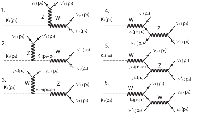
Figure 1: Feynman diagrams of the process $K^{+}\rightarrow\mu^{+}\nu_{\mu}\bar{\nu}_{l}\nu_{l}$. Similar diagrams contribute to the decay $K^{+}\rightarrow e^{+}\nu_{e}\bar{\nu}_{l}\nu_{l}$.

The amplitude of $K_{\mu 3\nu}$ can be written as

$${\cal M}=\frac{FG_{F}^{2}V_{us}}{\sqrt{2}}\times\sum_{i=1}^{6}M_{i}\equiv\frac{FG_{F}^{2}V_{us}}{\sqrt{2}}\times M\;,$$ (8)

where sum goes over all the six diagrams of Fig. 1 and we introduce the Fermi constant, $G_{F}\equiv g^{2}/4\sqrt{2}M_{W}^{2}$. The diagrams contribute to the amplitude as follows

$$M_{1}= 2\sin^{2}\theta\cdot\bar{\nu}_{l}(p_{1})\gamma^{\lambda}(1-\gamma_{5})\nu_{l}(p_{2})\cdot\bar{\nu}_{\mu}(p_{3})\gamma_{\lambda}(1-\gamma_{5})\mu(p_{4})$$

$$M_{2}= (1-2\sin^{2}\theta)\cdot\dfrac{(p_{3}+p_{4})^{\lambda}(p_{0}+p_{3}+p_{4})^{\rho}}{(p_{3}+p_{4})^{2}-M_{K}^{2}}\cdot\bar{\nu}_{l}(p_{1})\gamma_{\rho}(1-\gamma_{5})\nu_{l}(p_{2})\cdot\bar{\nu}_{\mu}(p_{3})\gamma_{\lambda}(1-\gamma_{5})\mu(p_{4})$$

$$M_{3}= -\frac{1}{2}\cdot\dfrac{(p_{1}+p_{2})^{\lambda}(p_{0}+p_{1}+p_{2})^{\rho}}{(p_{1}+p_{2})^{2}-M^{2}_{\alpha}}\cdot\bar{\nu}_{l}(p_{1})\gamma_{\lambda}(1-\gamma_{5})\nu_{l}(p_{2})\cdot\bar{\nu}_{\mu}(p_{3})\gamma_{\rho}(1-\gamma_{5})\mu(p_{4})$$

$$M_{4}= \frac{1}{2}\cdot\dfrac{1}{(p_{0}-p_{4})^{2}}p^{\rho}_{0}\cdot\bar{\nu}_{l}(p_{1})\gamma^{\lambda}(1-\gamma_{5})\nu_{l}(p_{2})\cdot\bar{\nu}_{\mu}(p_{3})\gamma_{\lambda}(1-\gamma_{5})(\hat{p}_{0}-\hat{p}_{4})\gamma_{\rho}(1-\gamma_{5})\mu(p_{4})$$

$$M_{5}= \frac{1}{2}\cdot p^{\lambda}_{0}\bar{\nu}_{\mu}(p_{3})\gamma_{\lambda}(1-\gamma_{5})\dfrac{-\hat{p}_{0}+\hat{p}_{3}+m_{\mu}}{(p_{0}-p_{3})^{2}-m_{\mu}^{2}}\gamma^{\rho}(4\sin^{2}\theta-1+\gamma_{5})\mu(p_{4})\cdot\bar{\nu}_{l}(p_{1})\gamma_{\rho}(1-\gamma_{5})\nu_{l}(p_{2})$$

$$M_{6}= p^{\rho}_{0}\cdot\bar{\nu}_{\mu}(p_{3})\gamma_{\lambda}(1-\gamma_{5})\mu(p_{4})\cdot\bar{\nu}_{l}\gamma^{\lambda}(1-\gamma_{5})\dfrac{m_{l}-\hat{p}_{0}+\hat{p}_{1}}{(p_{0}-p_{1})^{2}-m_{l}^{2}}\gamma^{\mu}(1-\gamma_{5})\nu_{l}(p_{2})$$

Similar amplitudes contribute to decay $K_{e3\nu}$ with obvious replacements $\mu(p_{4})\to e(p_{4})$, $\bar{\nu}_{\mu}(p_{3})\to\bar{\nu}_{e}(p_{3})$, and $m_{\mu}\to m_{e}$. In case of decay $K^{+}\rightarrow e^{+}\nu_{e}\nu_{\mu}\bar{\nu}_{\mu}$ diagram $6$ has resonance divergence associated with muon producing on-shell. We are dealing it by cutting out the phase space region, corresponding to $|(p_{0}-p_{1})^{2}-m_{\mu}^{2}|<(30\,\text{MeV})^{2}$.

3 Results and discussion

For the processes under discussion neutrinos can be treated as massless particles. Then amplitude $M_{3}$ referring to diagram 3 in Fig. 1 vanishes ($Z$ mixes with derivative of scalars, see lagrangian (7) which nullifies the amplitude for outgoing neutrinos on mass-shell). Also note, that for decays $K^{+}\rightarrow\mu^{+}\nu_{\mu}\bar{\nu}_{\mu}\nu_{\mu}$ and $K^{+}\rightarrow e^{+}\nu_{e}\bar{\nu}_{e}\nu_{e}$ there are two identical fermions in the final state and to the amplitudes presented in Sec. 2 must be added the same ones with opposite signs and changed momenta, $p_{1}\leftrightarrow p_{3}$. In appendix A explicit expressions for the squared amplitudes are presented. The phase space of the 4-body decays and integration over the momenta of outgoing fermions are discussed in appendix B. In Fig. 2

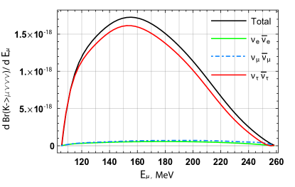
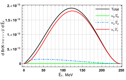
Figure 2: Lepton distributions over energy: Contributions of different final states (electron neutrino $\nu_{e}\bar{\nu}_{e}$, muon neutrino $\nu_{\mu}\bar{\nu}_{\mu}$ and tau-neutrino $\nu_{\tau}\bar{\nu}_{\tau}$ pairs) to the differential spectrum of muons from decays $K_{\mu 3\nu}$ (left panel) and to the differential spectrum of electrons from decays $K_{e3\nu}$ (right panel), normalized to the corresponding branching ratios.

we illustrate contributions of different channels to the differential spectrum of muons in $K_{\mu 3\nu}$ and electrons in $K_{e3\nu}$. As we can see contributions of the channel with $\tau$-neutrinos dominate. The difference is associated with the 6th diagram in Fig. 1, which is suppressed by the $\tau$-lepton mass. For other channels, the 6th diagram coming with relative negative sign reduces the sum of others. The details can be traced with formulas presented in appendix A(there the dominant and relevant for this issue coefficient is denoted as $A$).

The total lepton spectra, sums over all the three final states with different neutrino flavors, are presented in Fig. 2 as well. For experimental application we also show in Fig. 3

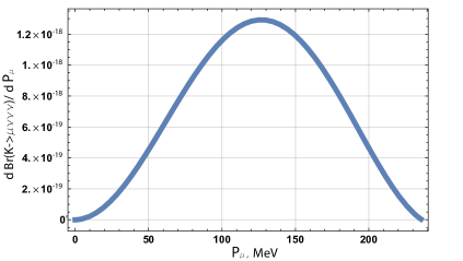
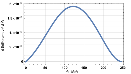
Figure 3: Momentum distribution of leptons normalized to the corresponding branching ratios: $K_{\mu 3\nu}$ (left), $K_{e3\nu}$ (right).

the lepton distributions over 3-momentum. By making use of the interpolating polynomials in lepton 3-momenta $p_{\mu}$($p_{e}$) [MeV] we find the following numerical fits to these distributions:

$$\begin{split}\frac{d\bf{Br}_{K_{\mu 3\nu}}}{dp_{\mu}}=&-2.893\times 10^{-22}+2.234\times 10^{-22}p_{\mu}+2.043\times 10^{-22}p_{\mu}^{2}+8.368\times 10^{-26}p_{\mu}^{3}\\ &-1.632\times 10^{-26}p_{\mu}^{4}+7.338\times 10^{-29}p_{\mu}^{5}-9.035\times 10^{-32}p_{\mu}^{6}\,,\end{split}$$ (9)

$$\begin{split}\frac{d\bf{Br}_{K_{e3\nu}}}{dp_{e}}=&-1.180\times 10^{-21}+1.040\times 10^{-20}p_{e}+1.990\times 10^{-22}p_{e}^{2}-4.793\times 10^{-25}p_{e}^{3}\\ &-1.328\times 10^{-26}p_{e}^{4}+6.474\times 10^{-29}p_{e}^{5}-7.752\times 10^{-32}p_{e}^{6}\,.\end{split}$$ (10)

The full branchings, obtained by integration of interpolating polynomials differ from those obtained by integration of exact ${\cal O}(p^{2})$ results by less than one percent.

Integrating over the muon (electron) momentum, one arrives at the following branching ratios:

$$\begin{array}[]{rclcrcl}{\rm Br}(K^{+}\rightarrow\mu^{+}\nu_{\mu}\nu_{\mu}\bar{\nu}_{\mu})&=&8.42\times 10^{-18}&&{\rm Br}(K^{+}\rightarrow e^{+}\nu_{e}\nu_{\mu}\bar{\nu}_{\mu})&=&2.00\times 10^{-17}\\ {\rm Br}(K^{+}\rightarrow\mu^{+}\nu_{\mu}\nu_{e}\bar{\nu}_{e})&=&6.27\times 10^{-18}&&{\rm Br}(K^{+}\rightarrow e^{+}\nu_{e}\nu_{e}\bar{\nu}_{e})&=&1.30\times 10^{-22}\\ {\rm Br}(K^{+}\rightarrow\mu^{+}\nu_{\mu}\nu_{\tau}\bar{\nu}_{\tau})&=&1.48\times 10^{-16}&&{\rm Br}(K^{+}\rightarrow e^{+}\nu_{e}\nu_{\tau}\bar{\nu}_{\tau})&=&2.38\times 10^{-16}\\ {\rm Br}(K^{+}\rightarrow\mu^{+}\nu_{\mu}\nu\bar{\nu})&=&1.62\times 10^{-16}&&{\rm Br}(K^{+}\rightarrow e^{+}\nu_{e}\nu\bar{\nu})&=&2.58\times 10^{-16}\end{array}$$

Obtained branchings are expectingly small and are beyond foreseeable direct registration (for instance NA$62$ at CERN is investigating the processes of $6$ orders higher branchings). The question arises, how to distinguish this weak process from others with similar observable signature. The full answer is certainly beyond the scope of this paper. An example of the irreducible background process is $K^{+}\rightarrow\pi^{+}\nu\bar{\nu}\rightarrow\mu^{+}\nu_{\mu}\nu\bar{\nu}$. Its contribution to the same final state as $K_{\mu 3\nu}$ in the finite volume detector can be discriminated by increasing the pion boost, which correspondingly suppress the probability of pion decay in flight. Moreover, the muon spectra exhibits different behavior, because the $\pi^{+}$ spectrum is growing throughout the whole kinematically allowed region Komatsubara (1999) (and therefore $\mu^{+}$ spectrum as well) while in $K^{+}\rightarrow\mu^{+}\nu_{\mu}\nu\bar{\nu}$ there is a clear maximum at $E_{\mu}\approx 155$ MeV. Thus although Br($K^{+}\rightarrow\pi^{+}\nu\bar{\nu}\rightarrow\mu^{+}\nu_{\mu}\nu\bar{\nu}$) $\approx 10^{6}Br(K^{+}\rightarrow\mu^{+}\nu_{\mu}\nu\bar{\nu})$, the study of low energy muons will give a chance to distinguish the two processes.

4 Conclusions

To summarise, exploiting the ChPT we perform to the leading order in momenta the calculation of lepton spectra and partial widths of kaon decays $K_{\mu 3\nu}$ and $K_{e3\nu}$. The accuracy of all numerical integrations and numerical fits to spectra are not worse than one percent. Recall, that the uncertainty associated with limiting the ChPT calculations by the leading order is significantly worse, about few tens percent.

We thank Yury Kudenko for suggesting to consider the problem of kaon four-body leptonic decay and encouraging conversations at various stages of the project. We thank Roman Lee and Artur Shaikhiev for discussions on the phase space integration. The work is supported by the RSF grant 14-22-00161.

Appendix A Squared amplitudes of $K_{\mu 3\nu}$ and $K_{e3\nu}$

In this section we present the explicit forms of squared matrix elements describing the four body decays $K_{\mu 3\nu}$ and $K_{e3\nu}$. To shorten the notations we denote the scalar product of $4$-vectors $p_{i}$ and $p_{j}$ as $p_{i}p_{j}\equiv x_{ij}$ (considering $i<j$ for definiteness). Then the corresponding squared amplitudes for decay $K_{\mu 3\nu}$ into the final states with electron and tau neutrinos, $l=e,\tau$, are

$$\begin{split}{M}^{2}=&\big{|}A\times\bar{\nu}_{l}(p_{1})\gamma^{\mu}(1-\gamma_{5})\nu_{l}(p_{2})\cdot\bar{\nu}_{\mu}(p_{3})\gamma_{\mu}(1-\gamma_{5})\mu(p_{4})+B\times\bar{\nu}_{l}(p_{1})\hat{p}_{0}(1-\gamma_{5})\nu_{l}(p_{2})\\ \times&\bar{\nu}_{\mu}(p_{3})(1+\gamma_{5})\mu(p_{4})+C\times\bar{\nu}_{l}(p_{1})\gamma_{\mu}(1-\gamma_{5})\nu(p_{2})\cdot\bar{\nu}_{\mu}(p_{3})\gamma_{\mu}(1-\gamma_{5})\hat{p}_{0}\mu(p_{4})\big{|}^{2}=\\ =&256A^{2}x_{13}x_{24}+64B^{2}x_{34}\left(2x_{01}x_{02}-x_{12}M_{K}^{2}\right)+256C^{2}\left(2x_{13}x_{02}x_{04}-M_{K}^{2}x_{13}x_{24}\right)\\ -&128ABm_{\mu}\left(x_{13}x_{02}+x_{01}x_{23}-x_{12}x_{03}\right)-512m_{\mu}ACx_{13}x_{02}+128BC\left[2x_{02}\left(x_{01}x_{34}\right.\right.\\ +&\left.\left.x_{13}x_{04}-x_{03}x_{14}\right)-M_{K}^{2}\left(x_{12}x_{34}+x_{13}x_{24}-x_{14}x_{23}\right)\right]\,,\end{split}$$ (11)

where

$$\begin{split}A&=2\left(\sin^{2}\theta+\frac{M_{K}^{2}-2x_{04}}{2(M_{K}^{2}-2x_{04}+m^{2}_{\mu})}-\frac{M_{K}^{2}-2x_{01}}{M_{K}^{2}-2x_{01}-m_{l}^{2}}\right.\\ &+\left.\left(\frac{1-2\sin^{2}\theta}{2}\right)\left(1+\frac{m_{\mu}^{2}}{2x_{12}+2x_{14}+2x_{24}}\right)\right),\\ B&=-2m_{\mu}\left(\dfrac{1-2\sin^{2}\theta}{2x_{12}-2x_{01}-2x_{02}}-\dfrac{2\sin^{2}\theta}{2x_{12}+2x_{14}+2x_{24}}\right),\\ C&=-m_{\mu}\left(\dfrac{1}{M_{K}^{2}-2x_{04}+m_{\mu}^{2}}+\dfrac{2\sin^{2}\theta}{2x_{12}+2x_{14}+2x_{24}}\right).\end{split}$$ (12)

Since $B$ and $C$ are proportional to mass of the charged lepton in the final state, in case of the decay $K_{e3\nu}$ they can be neglected. Then only one term in the squared matrix element survives, that is proportional to $A^{2}$, where one must replace $m_{\mu}$ with $m_{e}$.

Squared matrix elements for $K_{\mu 3\nu}$ with only muon neutrinos in the final set, $l=\mu$, read

$$\begin{split}{M}^{2}=&\big{|}A\times\bar{\nu}_{l}(p_{1})\gamma^{\lambda}(1-\gamma_{5})\nu_{l}(p_{2})\cdot\bar{\nu}_{\mu}(p_{3})\gamma_{\lambda}(1-\gamma_{5})\mu(p_{4})+B\times\bar{\nu}_{l}(p_{1})\hat{p}_{0}(1-\gamma_{5})\nu_{l}(p_{2})\\ \times&\bar{\nu}_{\mu}(p_{3})(1+\gamma_{5})\mu(p_{4})+C\times\bar{\nu}_{l}(p_{1})\gamma_{\lambda}(1-\gamma_{5})\nu(p_{2})\cdot\bar{\nu}_{\mu}(p_{3})\gamma^{\lambda}(1-\gamma_{5})\hat{p}_{0}\mu(p_{4})\\ +&D\times\bar{\nu}_{l}(p_{3})\hat{p}_{0}(1-\gamma_{5})\nu_{l}(p_{2})\cdot\bar{\nu}_{\mu}(p_{1})(1+\gamma_{5})\mu(p_{4})+E\times\bar{\nu}_{l}(p_{3})\gamma_{\lambda}(1-\gamma_{5})\nu(p_{2})\\ \times&\bar{\nu}_{\mu}(p_{1})\gamma^{\lambda}(1-\gamma_{5})\hat{p}_{0}\mu(p_{4})\big{|}^{2}=\\ =&256A^{2}x_{13}x_{24}+64B^{2}x_{34}\left(2x_{01}x_{02}-x_{12}M_{K}^{2}\right)+256C^{2}x_{13}\left(2x_{02}x_{04}-M_{K}^{2}x_{24}\right)\\ -&128ABm_{\mu}\left(x_{13}x_{02}+x_{01}x_{23}-x_{12}x_{03}\right)-512m_{\mu}ACx_{13}x_{02}+128BC\left[2x_{02}\left(x_{01}x_{34}\right.\right.\\ +&\left.\left.x_{13}x_{04}-x_{03}x_{14}\right)-M_{K}^{2}\left(x_{12}x_{34}+x_{13}x_{24}-x_{14}x_{23}\right)\right]+64D^{2}x_{14}\left(2x_{03}x_{02}-M_{K}^{2}x_{23}\right)\\ +&256E^{2}x_{13}\left(2x_{02}x_{04}-M_{K}^{2}x_{24}\right)-128m_{\mu}AD\left(x_{12}x_{03}+x_{13}x_{02}-x_{01}x_{23}\right)-512m_{\mu}AE\\ \times&x_{13}x_{02}-64BD\left[2x_{02}\left(x_{01}x_{34}+x_{14}x_{03}-x_{13}x_{04}\right)-M_{K}^{2}\left(x_{12}x_{34}+x_{14}x_{23}-x_{13}x_{24}\right)\right]\\ +&128BE\left[2x_{02}\left(x_{01}x_{34}+x_{13}x_{04}-x_{14}x_{03}\right)-M_{K}^{2}\left(x_{12}x_{34}+x_{13}x_{24}-x_{14}x_{23}\right)\right]\\ +&128CD\left[2x_{02}\left(x_{03}x_{14}+x_{13}x_{04}-x_{34}x_{01}\right)-M_{K}^{2}\left(x_{23}x_{14}+x_{13}x_{24}-x_{34}x_{12}\right)\right]\\ +&512CEx_{13}\left(2x_{04}x_{02}-M_{K}^{2}x_{24}\right)+128ED\left[2x_{02}\left(x_{03}x_{14}+x_{13}x_{04}-x_{34}x_{01}\right)\right.\\ -&\left.M_{K}^{2}\left(x_{23}x_{14}+x_{13}x_{24}-x_{34}x_{12}\right)\right]\end{split}$$ (13)

with

$$\begin{split}A=&2\left[\left(2\sin^{2}\theta+\frac{M_{K}^{2}-2x_{04}}{M_{K}^{2}-2x_{04}+m^{2}_{\mu}}\right)+\frac{1-2\sin^{2}\theta}{2}\left(2+\frac{m_{\mu}^{2}}{2x_{12}+2x_{14}+2x_{24}}\right.\right.\\ +&\left.\left.\frac{m_{\mu}^{2}}{2x_{23}+2x_{34}+2x_{24}}\right)-\left(\frac{M_{K}^{2}-2x_{01}}{M_{K}^{2}-2x_{01}-m_{\mu}^{2}}+\frac{M_{K}^{2}-2x_{03}}{M_{K}^{2}-2x_{03}-m_{\mu}^{2}}\right)\right]\\ B=&2m_{\mu}\left(\frac{2\sin^{2}\theta-1}{2x_{12}-2x_{01}-2x_{02}}+\frac{2\sin^{2}\theta}{2x_{12}+2x_{14}+2x_{24}}\right)\\ C=&-2m_{\mu}\left(\frac{1}{2(M_{K}^{2}-2x_{04}+m_{\mu}^{2})}+\frac{\sin^{2}\theta}{2x_{12}+2x_{14}+2x_{24}}\right)\\ D=&-2m_{\mu}\left(\frac{2\sin^{2}\theta-1}{2x_{23}-2x_{03}-2x_{02}}+\frac{2\sin^{2}\theta}{2x_{23}+2x_{34}+2x_{24}}\right)\\ E=&2m_{\mu}\left(\frac{1}{2(M_{K}^{2}-2x_{04}+m_{\mu}^{2})}+\frac{\sin^{2}\theta}{2x_{23}+2x_{34}+2x_{24}}\right)\end{split}$$ (14)

Again, in case of the decay $K_{e3\nu}$ all the coefficients above except $A$ and $E$ are proportional to mass of the charged lepton in the final state. Thus only the single term proportional to $A^{2}$ saturates the squared matrix element of $K_{e3\nu}$, and $m_{e}$ replaces $m_{\mu}$ in the expressions of $A$ presented above.

Appendix B Integration over the phase space of $K_{\mu 3\nu}$ and $K_{e3\nu}$

We examine the four particle decay and phase density of final states has relatively complicated from. The main idea is to examine a chain of two particle decays from the rest frame of kaon. Thus we write all momenta in the fixed frame from the very beginning. As a consequence of neutrinos being massless, momenta of decay products are unambiguous and resulting formula has a rather simple form.

In the following section we are using notation $p_{i}=(E_{i},\vec{p}_{i})$ for 4-vector $p_{i}$ and ${\bf p}$ for length of 3-vector $\vec{p}$. Formula of 2-particle phase space for decay $q\rightarrow q_{1}+q_{2}$ reads Byckling and Kajantie (1971)

$$R_{2}(q,q_{1},q_{2})=\frac{1}{4}\int d\Omega_{1}\sum_{a=+,-}(\textbf{q}_{1}^{a})^{2}(E\textbf{q}_{1}^{a}-\textbf{q}E_{1}^{a}\cos\theta)^{-1}\,,$$ (15)

where $\textbf{q}_{1}^{+,-}$ are solutions to the following equation,

$$E-E_{1}-(\textbf{q}^{2}+\textbf{q}_{1}^{2}-2\textbf{q q}_{1}\cos\theta_{1}+m_{2}^{2})^{1/2}=0\,,$$

so that $\cos\theta_{1}$ is angle between $\vec{q}$ and $\vec{q}_{1}$, $m_{2}^{2}=q_{2}^{2}$. The r.h.s. of eq. (15) contains Lorentz-non-invariant variables, but after integration $R_{2}$ still depends only on $q^{2}$ as it must be. Nevertheless we will denote it as $R_{2}(q,q_{1},q_{2})$ to specify particles, involved in decay.

Decomposition of n-particle phase space $R_{n}$ is performed with the following formula Byckling and Kajantie (1971)

$$R_{n}(M_{n}^{2})=\int_{\mu_{n-1}^{2}}^{(M_{n}-m_{n})^{2}}dM_{n-1}^{2}R_{2}(k_{n},k_{n-1},p_{n})R_{n-1}(M_{n-1}^{2})\,,$$ (16)

where $m_{i}=p_{i}^{2}$, $\mu_{i}\equiv\sum_{1}^{i}m_{i}$, $k_{i}\equiv\sum_{1}^{i}p_{i}$, $M_{n}^{2}=k_{n}^{2}$. Thus, applying the reduction formula (16) twice, substituting common $R_{2}$ expressions and integrating out $3$ trivial angles, we arrive at the following master formula

$$\begin{split}R_{4}(M_{K}^{2})=\frac{\pi^{2}}{8}\int^{(M_{K}-m_{4})^{2}}_{0}dM^{2}_{3}\int^{M_{3}^{2}}_{0}dM_{2}^{2}\int_{-1}^{1}d\cos\theta_{1}\int_{-1}^{1}d\cos\theta_{2}\int_{0}^{2\pi}d\phi\\ \times\frac{[(M_{K}^{2}-(M_{3}+m_{4})^{2})(M_{K}^{2}-(M_{3}-m_{4})^{2})]^{1/2}\times\textbf{p}_{3}^{2}\times\textbf{p}_{2}^{2}}{2M_{K}^{2}\times(E_{123}\textbf{p}_{3}-\textbf{p}_{123}E_{3}\cos\theta_{1})\times(E_{12}\textbf{p}_{2}-\textbf{p}_{12}E_{2}\cos\theta_{2})}\,.\end{split}$$ (17)

Here we adopt the useful auxiliary momentum variables $p_{12}=(E_{12},\vec{p}_{12})=p_{1}+p_{2}$; $p_{123}=(E_{123},\vec{p}_{123})=p_{1}+p_{2}+p_{3}$, so that $M^{2}_{2}=p_{12}^{2}$, $M^{2}_{3}=p_{123}^{2}$, and angle variables $\theta_{1}\equiv\angle(\vec{p}_{3}\,,\vec{p}_{123})$, $\theta_{2}\equiv\angle(\vec{p}_{2},\vec{p}_{12})$, $\phi$ is rotation angle of plane $(\vec{p}_{12}\,,\vec{p}_{2})$ around $\vec{p}_{12}$, as demonstrated in Fig. 4.

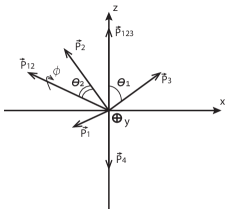
Figure 4: Definition of integration variables (2D sketch).

The decay rates of $K_{l3\nu}$ are found by integrating the corresponding squared amplitudes (8) over the above defined phase space,

$$\Gamma_{K_{l3\nu}}=\int\frac{1}{2M_{K}(2\pi)^{8}}\left|{\cal M}\right|^{2}dR_{4}\,,$$ (18)

in the cases with two identical neutrinos in final state we must also divide the obtained in this way result by $2$. Now substituting $M_{3}^{3}=(p_{0}-p_{4})^{2}$ it is straightforward to obtain the differential spectra:

$$\begin{split}\frac{d\Gamma_{K_{l3\nu}}}{d{\bf p_{4}}}=\frac{1}{(2\pi)^{6}}\int^{M_{3}^{2}}_{0}dM_{2}^{2}\int_{-1}^{1}d\cos\theta_{1}\int_{-1}^{1}d\cos\theta_{2}\int_{0}^{2\pi}d\phi\\ \times\frac{[(M_{K}^{2}-(M_{3}+m_{4})^{2})(M_{K}^{2}-(M_{3}-m_{4})^{2})]^{1/2}\times\textbf{p}_{3}^{2}\times\textbf{p}_{2}^{2}}{2M_{K}^{2}\times(E_{123}\textbf{p}_{3}-\textbf{p}_{123}E_{3}\cos\theta_{1})\times(E_{12}\textbf{p}_{2}-\textbf{p}_{12}E_{2}\cos\theta_{2})}\times\frac{\textbf{p}_{4}\left|{\cal M}\right|^{2}}{32E_{4}}\,,\end{split}$$ (19)

where $M_{3}^{2}=M_{K}^{2}+m_{4}^{2}-2M_{K}E_{4}$. Then the branching fraction is defined as

$$\text{Br}_{K_{l3\nu}}\equiv\tau_{K}\cdot\Gamma_{K_{l3\nu}}\,,$$

where $\tau_{K}$ is the kaon lifetime. For the numerical estimates we substitute the kaon decay constant $F_{K}\approx 111$ MeV Olive et al. (2014) for the meson decay constant $F$.

References

- Gasser and Leutwyler (1982) J. Gasser and H. Leutwyler, Phys. Rept. 87, 77 (1982).
- Cable et al. (1972) G. D. Cable, R. H. Hildebrand, C. Y. Pang, and R. Stiening, Phys. Lett. B40, 699 (1972).
- Pang et al. (1973) C. Y. Pang, R. H. Hildebrand, G. D. Cable, and R. Stiening, Phys. Rev. D8, 1989 (1973).
- Artamonov et al. (2015) A. V. Artamonov et al. (E949), Phys. Rev. D91, 052001 (2015), [Erratum: Phys. Rev.D91,no.5,059903(2015)], arXiv:1411.3963 [hep-ex] .
- Gorbunov and Shaposhnikov (2007) D. Gorbunov and M. Shaposhnikov, JHEP 10, 015 (2007), [Erratum: JHEP11,101(2013)], arXiv:0705.1729 [hep-ph] .
- Beranek and Vanderhaeghen (2013) T. Beranek and M. Vanderhaeghen, Phys. Rev. D87, 015024 (2013), arXiv:1209.4561 [hep-ph] .
- Pospelov et al. (2008) M. Pospelov, A. Ritz, and M. B. Voloshin, Phys. Lett. B662, 53 (2008), arXiv:0711.4866 [hep-ph] .
- Bardin et al. (1970) D. Yu. Bardin, S. M. Bilenky, and B. Pontecorvo, Phys. Lett. B32, 121 (1970).
- Bijnens et al. (1994) J. Bijnens, G. Ecker, and J. Gasser, in 2nd DAPHNE Physics Handbook:125-144 (1994) pp. 125–144, arXiv:hep-ph/9411232 [hep-ph] .
- Komatsubara (1999) T. K. Komatsubara (E787, E949), in Weak interactions and neutrinos. Proceedings, 17th International Workshop, WIN’99, Cape Town, South Africa, January 24-30, 1999 (1999) pp. 535–539, arXiv:hep-ex/9905014 [hep-ex] .
- Byckling and Kajantie (1971) E. Byckling and K. Kajantie, Particle Kinematics (University of Jyvaskyla, Jyvaskyla, Finland, 1971).
- Olive et al. (2014) K. A. Olive et al. (Particle Data Group), Chin. Phys. C38, 090001 (2014).