A manifestly Hermitian semiclassical expansion for the one-particle density matrix of a two-dimensional Fermi gas

Abstract

The semiclassical $\hbar$-expansion of the one-particle density matrix for a two-dimensional Fermi gas is calculated within the Wigner transform method of Grammaticos and Voros, originally developed in the context of nuclear physics. The method of Grammaticos and Voros has the virture of preserving both the Hermiticity and idempotency of the density matrix to all orders in the $\hbar$-expansion. As a topical application, we use our semiclassical expansion to go beyond the local-density approximation for the construction of the total dipole-dipole interaction energy functional of a two-dimensional, spin-polarized dipolar Fermi gas. We find a finite, second-order gradient correction to the Hartree-Fock energy, which takes the form $\varepsilon(\nabla\rho)^{2}/\sqrt{\rho}$, with $\varepsilon$ being small ($|\varepsilon|\ll 1$) and negative. We test the quality of the corrected energy by comparing it with the exact results available for harmonic confinement. Even for small particle numbers, the gradient correction to the dipole-dipole energy provides a significant improvement over the local-density approximation.

I Introduction

Density-functional theory (DFT) DFT is by far the most common and powerful numerical approach for the solution of the quantum many-body problem of $N$ interacting fermions, and constitutes the cornerstone for research in diverse fields such as condensed matter and nuclear physics, quantum chemistry, and materials science. Specifically, the Hohenberg-Kohn-Sham (HKS) DFT DFT states that the ground state properties of an $N$-body interacting Fermi system may be mapped to a noninteracting system of independent fermions moving in an effective one-body potential, $v_{\rm eff}({\bf r})$, sometimes referred to as the Kohn-Sham potential, $v_{\rm KS}({\bf r})$. The HKS total energy functional is then given by (hereby, we focus to strictly two-dimensional (2D) systems)

$$E[\rho]=T_{0}[\rho]+E_{\rm int}[\rho]+\int d^{2}r~{}v_{\rm ext}({\bf r})\rho({\bf r})~{}.$$ (1)

In Eq. (1), $T_{0}[\rho]$ is the kinetic energy (KE) of a noninteracting Fermi gas, $E_{\rm int}[\rho]$ accounts for both classical and quantum interactions, and the last term is the energy functional associated with the external potential, $v_{\rm ext}({\bf r})$.

The noninteracing KE functional is treated exactly in the HKS formalism, and by definition is given by (in this paper, we deal with fermions with spin degeneracy $g=1,2$)

$$T_{0}[\rho]=g\sum_{i=1}^{N/g}\int d^{2}r~{}\phi_{i}^{*}({\bf r})\left(-\frac{\hbar^{2}}{2m}\nabla^{2}\right)\phi_{i}({\bf r})~{},$$ (2)

where the summation is over fully occupied orbitals, $\{\phi_{i}({\bf r})\}$. The variational minimization of $E[\rho]$ with respect to the density then leads to the following set of single-particle Schrödinger-like equation for the orbitals, $\{\phi_{i}({\bf r})\}$,

$$-\frac{\hbar^{2}}{2m}\nabla^{2}\phi_{i}({\bf r})+v_{\rm eff}({\bf r})\phi_{i}({\bf r})=\varepsilon_{i}\phi_{i}({\bf r})~{},~{}~{}~{}~{}(i=1,...,N)~{},$$ (3)

where the effective potential mentioned above is given by

$$v_{\rm eff}({\bf r})=\frac{\delta E_{\rm int}[\rho]}{\delta\rho}+v_{\rm ext}({\bf r})~{}.$$ (4)

Therefore, in the HKS scheme, one must self-consistently solve for $N$ Schrödinger-like equations, which at self-consistency leads to the spatial density

$$\rho({\bf r})=g\sum_{i=1}^{N/g}\phi_{i}^{*}({\bf r})\phi_{i}({\bf r})~{},$$ (5)

with the normalization,

$$\int d^{2}r~{}\rho({\bf r})=N~{},$$ (6)

also determining the Fermi energy, $E_{F}$.

The interaction energy functional, $E_{\rm int}[\rho]$, is generally not known, so some approximation must be made for $E_{\rm int}[\rho]$ in order to completely specify the HKS functional, Eq. (1). Despite its conceptual appeal, any practical implementation of the HKS theory, as defined above, must be weighed against the numerically expensive self-consistent solution to $N$ single-particle Schrödinger-like equations, Eq. (3).

Ideally, one would like to keep in the original spirit of DFT, in which there is no need for the calculation of single-particle orbitals of any kind. In principle, this so-called orbital-free DFT can be accomplished within the HKS scheme if one could construct an explicit density functional for the exact, noninteracting KE, $T_{0}[\rho]$, for an arbitrary inhomogeneous system. To date, such a functional has not been found, implying that if one would like to avoid calculating single-particle orbitals, an additional layer of approximation must be made; that is, in an orbital-free DFT, two functionals, $T_{0}[\rho]$ and $E_{\rm int}[\rho]$, must be approximated. Nevertheless, if the approximation to $T_{0}[\rho]$ is accurate, the computational cost savings for investigating $N\gg 1$ systems is extremely compelling, and is often the only practical numerical option (e.g., in materials science, where $N\sim{\cal O}(10^{23})$).

Toward the goal of obtaining an expression for the KE functional, $T_{0}[\rho]$, explicitly in terms of the spatial density, one may introduce the one-body density matrix (ODM), which is formally defined in terms of the normalized many-body wave function DFT , $\psi$, viz.,

$$\rho_{1}({\bf r};{\bf r}^{\prime})=N\int d^{2}r_{2}...d^{2}r_{N}~{}\psi^{*}({\bf r},{\bf r}_{2},...,{\bf r}_{N})\psi({\bf r}^{\prime},{\bf r}_{2},...,{\bf r}_{N})~{}.$$ (7)

Note that by definition, the spatial density is given by the diagonal element of the ODM, viz., $\rho({\bf r})=\rho_{1}({\bf r};{\bf r})$, along with the fact that the ODM is Hermitian, $\rho_{1}({\bf r};{\bf r}^{\prime})=[\rho_{1}({\bf r}^{\prime};{\bf r})]^{*}$ . It will prove advantageous later to introduce the center-of-mass and relative coordinates, ${\bf R}=({\bf r}+{\bf r}^{\prime})/2$ and ${\bf s}={\bf r}-{\bf r}^{\prime}$, respectively. We also define

$$\bar{\rho}_{1}({\bf R};{\bf s})\equiv\rho_{1}({\bf R}+{\bf s}/2;{\bf R}-{\bf s}/2)~{},$$ (8)

in which case Hermiticity takes the form $\bar{\rho}_{1}({\bf R};{\bf s})=[\bar{\rho}_{1}({\bf R};-{\bf s})]^{*}$ The noninteracting KE functional is then obtained from

$$T_{0}[\rho]=-\frac{\hbar^{2}}{2m}\int d^{2}R~{}[\nabla^{2}_{\bf s}\bar{\rho}_{1}({\bf R};{\bf s})]_{{\bf s}=0}.$$ (9)

Unsurprisingly, there is no known explicit expression for the ODM for an arbitrary inhomogeneous system, implying that approximations to the ODM are unavoidable. It is evident that the quality of any approximation to the noninteracting KE functional is inextricably connected with the approximation applied to the ODM.

The crudest expression for $\bar{\rho}_{1}({\bf R};{\bf s})$ is the so-called local-density approximation (LDA) in which the form of the ODM of a spatially uniform 2D system is assumed to be locally valid for an inhomogeneous system brack_bhaduri ; vanzyl2003 ,viz.,

$$\bar{\rho}_{1}({\bf R};{\bf s})=g\frac{k_{F}({\bf R})^{2}}{2\pi}\frac{J_{1}[k_{F}({\bf R})|{\bf s}|]}{k_{F}({\bf R})|{\bf s}|}~{},$$ (10)

where $k_{F}({\bf R})=\sqrt{4\pi\rho({\bf R})/g}$ is the local Fermi wave vector and $J_{n}(x)$ is a cylindrical Bessel function of the $n$-th order GR . It is immediately seen that Eq. (10) is Hermitian. Note that in, e.g., the Kirzhnits commutator formalism DFT , the fact that one begins with a representation in ${\bf r}$ and ${\bf r}^{\prime}$, means that the resulting Kirzhnits LDA for the ODM is not Hermitian. Specifically, in the Kirzhnits approach, one obtains

$${\rho}_{1}({\bf r};{\bf r}^{\prime})=g\frac{k_{F}({\bf r})^{2}}{2\pi}\frac{J_{1}[k_{F}({\bf r})|{\bf s}|]}{k_{F}({\bf r})|{\bf s}|}~{},$$ (11)

which clearly does not possess the correct ${\bf r}$ and ${\bf r}^{\prime}$ symmetry. However, upon the appropriate symmetrization, one is lead to an expression identical to Eq. (10).

Inserting Eq. (10) into Eq. (9) leads to the LDA for the noninteracting kinetic energy functional, viz.,

$$T_{0}[\rho]=\frac{\pi}{g}\frac{\hbar^{2}}{m}\int d^{2}R~{}\rho({\bf R})^{2}~{},$$ (12)

which is obviously an explicit functional of the spatial density. Presumably, going beyond the LDA for the ODM will lead to a more accurate noninteracting KE functional. We will come back to this point later in the paper.

The interaction energy functional, $E_{\rm int}[\rho]$, may also be determined solely in terms of the ODM if one adopts the common Hartree-Fock approximation (HFA), which does not take into account correlations, viz.,

$$E_{\rm int}[\rho]=\int\int d^{2}rd^{2}r^{\prime}~{}\frac{1}{2}\left(\rho_{1}({\bf r},{\bf r})\rho_{1}({\bf r}^{\prime},{\bf r}^{\prime})-\frac{1}{g}\rho_{1}({\bf r},{\bf r}^{\prime})\rho_{1}({\bf r}^{\prime},{\bf r})\right)v_{\rm int}({\bf r},{\bf r}^{\prime})~{},$$ (13)

where $v_{\rm int}({\bf r},{\bf r}^{\prime})$ is the two-body interaction potential (e.g., a $1/|{\bf r}-{\bf r}^{\prime}|$ Coulomb potential). The first term in Eq. (13) corresponds to the classical Hartree energy, while the second term represents the quantum-mechanical exchange energy. We then see that the ODM is not only fundamental for obtaining the noninteracting KE functional, but also (at least within the HFA) the interaction energy functional. Unfortunately, to our knowledge, the only inhomogeneous systems for which an exact analytical expresion for the ODM is available are the so-called Bardeen model bardeen , the three-dimensional harmonic oscillator (HO) with smeared occupancy bhaduri , and the multi-dimensional HO vanzyl2003 ; march . The point to be taken here is that if one wishes to find explicit functionals for $T_{0}[\rho]$, and $E_{\rm int}[\rho]$, approximations to the ODM must be employed, since $\rho_{1}({\bf r};{\bf r}^{\prime})$ is not known exactly for an arbitrary inhomogenous system.

To this end, in Sec. II, we briefly review the Grammaticos-Voros (GV) semiclassical (SC) $\hbar$-expansion for the ODM GM , and subsequently apply it to develop a Hermitian, idempotent, $\hbar$-expansion for the 2D density matrix of an arbitrary inhomogeneous 2D Fermi gas. While an analogous calculation of this kind (i.e., using the GV approach) has been recently performed by Bencheikh and Räsänen BR in three-dimensions (3D), we feel that a presentation of the 2D analysis is a worthwhile endeavor. First, from a pedagogical point of view, the calculations involved in obtaining the SC 2D ODM are somewhat unwieldy, so providing the details of such calculations will be useful to other researchers wishing to apply, or extend our results. In addition, providing an explicit expression for the SC 2D ODM is of academic interest, since its presentation utilizing the GV approach is currently not available in the literature. Finally, the fundamental role of the ODM in applications of DFT to degenerate Fermi gases, suggests that our work will also be of practical importance in diverse areas of research (e.g., instabilities in 2D dipolar Fermi gases (dFG), Wigner crystallization in 2D electronic and dFG, physics of metal clusters, etc).

Following this development, we will apply our results to construct a beyond the LDA expression for the total HF dipole-dipole interaction energy for a 2D spin-polarized dipolar Fermi gas. Our paper closes with a summary and suggestions for future work.

II Semiclassical $h$-bar expansion of the density matrix

We begin by considering a 2D system of noninteracting fermions under the influence of some one-body potential,

$$\hat{H}=-\frac{\hbar^{2}}{2m}\nabla^{2}+V({\bf r})$$ (14)

along with the associated one-particle density operator

$$\hat{\rho}=\Theta(E_{F}-\hat{H})~{},$$ (15)

where $E_{F}$ is the Fermi energy and $\Theta$ is the Heaviside function.

We develop our semiclassical expansion by working with the Wigner transform of $\rho_{1}({\bf r};{\bf r}^{\prime})$, as originally developed by GV GM and recently applied to the 3D ODM by Bencheikh and Räsänen BR viz.,

$$\bar{\rho}^{\rm sc}_{1}({\bf R};{\bf s})=\frac{1}{(2\pi\hbar)^{2}}\int d^{2}p~{}\rho^{\rm sc}_{\rm w}({\bf R},{\bf p})e^{i{\bf p}\cdot{\bf s}/\hbar}~{},$$ (16)

where ${\bf p}$ is the momentum conjugate to ${\bf s}$, and $\rho_{\rm w}({\bf R},{\bf p})$ denotes the Wigner transform of $\rho_{1}({\bf r};{\bf r}^{\prime})$. Note that in the GV approach, one immediately works in the ${\bf R}$ and ${\bf s}$ representation, which then leads to a transparent expression from which one can deduce the Hermiticity of the ODM.

At the heart of the method is to expand $\rho_{\rm w}({\bf R},{\bf p})=[\theta(E_{F}-\hat{H})]_{\rm w}$ around the identity operator times the classical Hamiltonian $H_{\rm cl}$,

$$H_{\rm cl}=\frac{{\bf p}^{2}}{2m}+V({\bf R})~{}.$$ (17)

To second order in $\hbar$, one finds the dimensionally independent expression for $\rho^{\rm sc}_{\rm w}({\bf R},{\bf p})$, which reads GM ; BR

$$\rho^{\rm sc}_{\rm w}({\bf R},{\bf p})=\Theta(E_{F}-H_{\rm cl})-\frac{1}{2}\varphi_{2}\delta^{\prime}(H_{\rm cl}-E_{F})-\frac{1}{6}\varphi_{3}\delta^{\prime\prime}(H_{\rm cl}-E_{F})+{\cal O}(\hbar^{4})~{},$$ (18)

$$\varphi_{2}=-\frac{\hbar^{2}}{4m}\nabla^{2}_{\bf R}V+{\cal O}(\hbar^{4})~{},$$ (19)

and

$$\varphi_{3}=-\frac{\hbar^{2}}{4m}\left[(\nabla_{\bf R}V)^{2}+\frac{1}{m}({\bf p}\cdot\nabla_{\bf R})^{2}V\right]+{\cal O}(\hbar^{4})~{},$$ (20)

where primes refer to derivatives with respect to $H_{\rm cl}$ note1 . The semiclassical $\hbar$-expansion of the ODM is then obtained by inserting Eq. (18), along with the expressions for $\varphi_{2}$ and $\varphi_{3}$ into Eq. (16), viz.,

$$\bar{\rho}^{\rm sc}_{1}({\bf R};{\bf s})=(A+B+C+D)~{},$$ (21)

where we recall that $\bar{\rho}_{1}({\bf R};{\bf s})\equiv\rho_{1}({\bf R}+\frac{1}{2}{\bf s};{\bf R}-\frac{1}{2}{\bf s})$, and

$$A = \frac{g}{(2\pi\hbar)^{2}}\int d^{2}p~{}e^{i{\bf p}\cdot{\bf s}/\hbar}\Theta(E_{F}-H_{\rm cl})~{},$$ (22)

$$B = \frac{g}{(2\pi\hbar)^{2}}\frac{\hbar^{2}}{8m}\nabla_{\bf R}^{2}V\int d^{2}p~{}e^{i{\bf p}\cdot{\bf s}/\hbar}\delta^{\prime}(H_{\rm cl}-E_{F})~{},$$ (23)

$$C = \frac{g}{(2\pi\hbar)^{2}}\frac{\hbar^{2}}{24m}(\nabla_{\bf R}V)^{2}\int d^{2}p~{}e^{i{\bf p}\cdot{\bf s}/\hbar}\delta^{\prime\prime}(H_{\rm cl}-E_{F})~{},$$ (24)

$$D = \frac{g}{(2\pi\hbar)^{2}}\frac{\hbar^{2}}{24m^{2}}\int d^{2}p~{}e^{i{\bf p}\cdot{\bf s}/\hbar}({\bf p}\cdot\nabla_{\bf R})^{2}V\delta^{\prime\prime}(H_{\rm cl}-E_{F})~{}.$$ (25)

The analytical evaluation of the above integrals requires the following identities (below, $p_{F}=\hbar k_{F}$) ,

$$\delta(H_{\rm cl}-E_{F})=\frac{m}{p_{F}}\delta(p-p_{F})~{},$$ (26)

$$\frac{d\delta(H_{\rm cl}-E_{F})}{dH_{\rm cl}}=\frac{m^{2}}{p_{F}p}\frac{d\delta(p-p_{F})}{dp}~{},$$ (27)

and

$$\frac{d^{2}\delta(H_{\rm cl}-E_{F})}{dH_{\rm cl}^{2}}=\frac{m^{3}}{p_{F}}\left[\frac{1}{p^{2}}\frac{d^{2}\delta(p-p_{F})}{dp^{2}}-\frac{1}{p^{3}}\frac{d\delta(p-p_{F})}{dp}\right]~{}.$$ (28)

Each of the integrals, $A,B,C,D$, is explicitly worked out in Appendices A–D. Here, we will simply write down our final result for the semi-classical $\hbar$-expansion of the ODM (to ${\cal O}(\hbar^{2})$) note ,

$$\bar{\rho}^{\rm sc}_{1}({\bf R};{\bf s}) = g\left\{\frac{k_{F}^{2}}{2\pi}\frac{J_{1}(z)}{z}-\frac{1}{48\pi}zJ_{1}(z)\frac{\nabla^{2}_{\bf R}k_{F}^{2}}{k_{F}^{2}}+\frac{1}{96\pi}\frac{z^{2}J_{0}(z)}{k_{F}^{2}}\left[\nabla_{\bf R}\left(\nabla_{\bf R}k_{F}^{2}\cdot\frac{{\bf s}}{s}\right)\cdot\frac{{\bf s}}{s}\right]\right.$$ (29)

$$+ \left.\frac{1}{192\pi}z^{2}J_{2}(z)\frac{(\nabla_{\bf R}k_{F}^{2})^{2}}{k_{F}^{4}}\right\}~{},$$

where $z=k_{F}|{\bf s}|$ and $k_{F}({\bf R})=\sqrt{2m(E_{F}-V({\bf R})/\hbar^{2}}$ is the local Fermi wave vector. The first term in $\bar{\rho}^{\rm sc}_{1}({\bf R};{\bf s})$ agrees exactly with Eq. (10), and highlights that the lowest order contribution to Eq. (29) corresponds to the LDA, or equivalently, the Thomas-Fermi approximation. As promised, the GV ODM is manifestly Hermitian, and takes a very different form to the Kirzhnits ODM recently derived by Putaja et al. Putaja ; note3 .

II.1 The spatial and kinetic energy densities

The semiclassical spatial density is immediately obtained by taking the diagonal element of Eq. (29). However, all terms but the first vanish in taking the ${\bf s}\to 0$ limit (i.e. ${\bf R}\to{\bf r}$), and one obtains,

$$\rho^{\rm sc}({\bf R})=g\frac{[k_{F}({\bf R})]^{2}}{4\pi}~{},$$ (30)

which is just the LDA applied to the uniform gas. This result is special to 2D, since in 1D and 3D, non-vanishing gradient corrections are present Putaja ; kirz ; sala ; koivisto .

The KE density may be found by inserting Eq. (29) into Eq. (9), but upon taking the ${\bf s}\to 0$ limit, all but the LDA term will vanish, leaving

$$T_{0}[\rho]=\frac{\pi}{g}\frac{\hbar^{2}}{m}\int d^{2}R~{}\rho({\bf R})^{2}~{}.$$ (31)

Again, the GV expansion of the ODM has not changed the fact that there are no gradient corrections to the noninteracting KE functional for an inhomogeneous 2D Fermi gas; that is, the KE functional is the Thomas-Fermi functional for a 2D noninteracting Fermi gas which is again unique to 2D systems Putaja ; kirz ; sala ; koivisto . Gradient corrections to the 2D KE functional can be motivated within the so-called average density approximation, but this requires the KE functional to be inherently nonlocal vanzylADA .

II.2 Consistency criterion of the Euler equation and Idempotency

Coming first to the consistency criterion established by Gross and Proetto gross , it has already been shown in Ref. Putaja that the Thomas-Fermi KE density functional satisfies the Euler equation that minimizes the total energy functional, Eq. (1),

$$\frac{\delta T_{0}[\rho]}{\delta\rho}+v_{\rm eff}({\bf r})=E_{F}~{}.$$ (32)

Owing to the fact that in the GV formulation, only the Thomas-Fermi term survives, consistency is guaranteed.

The idempotency of the GV semiclassical ODM has already been proved in arbitrary dimensions in Ref. BR . It follows that our 2D ODM, Eq. (29), is also idempotent, which is in fact a strong constraint to be placed on any approximate density matrix.

III Application: 2D spin-polarized dipolar Fermi gas

In this section, we will use our semiclassical expansion for the ODM, Eq. (29), to go beyond the LDA for the total dipole-dipole interaction energy functional of a spin-polarized (all moments aligned parallel with the $z$-axis), inhomogeneous 2D dipolar Fermi gas. We restrict ourselves to the HFA, where the total dipolar interaction energy is given by

$$E_{\rm int}=\frac{1}{2}\int d^{2}r\int d^{2}r^{\prime}~{}[\rho_{1}({\bf r};{\bf r})\rho_{1}({\bf r}^{\prime};{\bf r}^{\prime})-\rho_{1}({\bf r};{\bf r}^{\prime})\rho_{1}({\bf r}^{\prime};{\bf r})]V_{dd}({\bf r}-{\bf r}^{\prime})~{},$$ (33)

and

$$V_{dd}({\bf r}-{\bf r}^{\prime})=\frac{\mu_{0}d^{2}}{4\pi}\frac{1}{|{\bf r}-{\bf r}^{\prime}|^{3}}~{},$$ (34)

is the interaction potential between two magnetic dipoles restricted to locations ${\bf r}$ and ${\bf r}^{\prime}$ in the 2D $xy$-plane, and $d$ is the magnetic moment of an atom. The individual terms in Eq. (33) are the direct and exchange energies, and while they are separately divergent for a $1/r^{3}$ potential in 2D, their sum is finite owing to the Pauli exclusion principle vanzyl_pisarski . As discussed at length in Ref. vanzyl_pisarski , it is convenient to work with a regularized dipolar interaction, which leads to the following expression for the total interaction energy within the HFA (details of this calculation have already been presented in Ref. vanzyl_pisarski ),

$$E_{\rm int} = \frac{\mu_{0}d^{2}}{8\pi}\int d^{2}s~{}\frac{1}{s^{3}}[f(0)-f({\bf s})]-\frac{\mu_{0}d^{2}}{4}\int\frac{d^{2}q}{(2\pi)^{2}}~{}q|\tilde{\rho}({\bf q})|^{2}$$ (35)

$$\equiv E^{(1)}_{dd}+E^{(2)}_{dd}~{}.$$

where $\tilde{\rho}({\bf q})$ is the 2D Fourier transform of the density, and

$$f(0)-f({\bf s})=\int d^{2}R\{[\bar{\rho}_{1}({\bf R};0)]^{2}-[\bar{\rho}_{1}({\bf R};{\bf s})]^{2}\}~{}.$$ (36)

It is important to emphasize here that $E^{(1)}_{dd}$ and $E^{(2)}_{dd}$ are not to be interpreted as the direct and exchange energies, respectively. Note that $E^{(2)}_{dd}$ is the nonlocal contribution to the HF energy, and as written is exact. On the other hand, in order to get an explicit expression for $E^{(1)}_{dd}$ in terms of the density, we need to invoke some level of approximation to $f(0)-f({\bf s})$.

To this end, we define the radial distribution function for the inhomogeneous system as

$$g({\bf R};{\bf s})=1-\frac{[\bar{\rho}_{1}({\bf R};{\bf s})]^{2}}{[\bar{\rho}_{1}({\bf R};0)]^{2}}~{},$$ (37)

so that we may write

$$E^{(1)}_{dd}=\frac{\mu_{0}d^{2}}{8\pi}\int d^{2}R\int d^{2}s\frac{1}{s^{3}}[\rho({\bf R})]^{2}g({\bf R};{\bf s})~{}.$$ (38)

Now, taking only the leading order term from our semiclassical expansion of the ODM, Eq. (29) ($g=1$), we immediately obtain

$$E^{(1),{\rm LDA}}_{dd} = \frac{\mu_{0}d^{2}}{4}\int d^{2}R[\rho({\bf R})]^{2}k_{F}({\bf R})\int_{0}^{\infty}dz\frac{1}{z^{2}}\left[1-\left(\frac{2J_{1}(z)}{z}\right)^{2}\right]$$ (39)

$$= \mu_{0}d^{2}\frac{\sqrt{\pi}}{2}\int d^{2}R[\rho({\bf R})]^{5/2}\frac{128}{45\pi}$$

$$= \mu_{0}d^{2}\frac{64}{45\sqrt{\pi}}\int d^{2}R~{}[\rho({\bf R})]^{5/2}~{},$$

which is in perfect agreement with Eq. (27) in Ref. vanzyl_pisarski .

We may now go beyond the LDA for $E^{(1)}_{dd}$ by taking in turn all of the $\hbar^{2}$ corrections to the ODM in Eq. (29). To begin, we note that to ${\cal O}(\hbar^{2})$

$$|\bar{\rho}_{1}^{\rm sc}({\bf R};{\bf s})|^{2} = \frac{k_{F}^{4}}{4\pi^{2}}\left(\frac{J_{1}(z)}{z}\right)^{2}+\frac{zJ_{1}(z)J_{2}(z)}{192\pi^{2}}\frac{(\nabla_{\bf R}k_{F}^{2})^{2}}{k_{F}^{2}}-\frac{(J_{1}(z))^{2}}{48\pi^{2}}(\nabla_{\bf R}^{2}k_{F}^{2})$$ (40)

$$+ \frac{zJ_{1}(z)J_{0}(z)}{96\pi^{2}}\left[\nabla_{\bf R}\left(\nabla_{\bf R}k_{F}^{2}\cdot\frac{{\bf s}}{s}\right)\cdot\frac{{\bf s}}{s}\right]~{},$$

from which we obtain

$$g^{\rm sc}({\bf R};{\bf s}) = 1-\frac{[\bar{\rho}_{1}^{\rm sc}({\bf R};{\bf s})]^{2}}{[\rho({\bf R})]^{2}}$$ (41)

$$= \left[1-\left(\frac{2J_{1}(z)}{z}\right)^{2}\right]-\frac{zJ_{1}(z)J_{2}(z)}{48\pi}\frac{(\nabla_{\bf R}\rho)^{2}}{\rho^{3}}+\frac{1}{48\pi^{2}}\frac{\nabla^{2}_{\bf R}k^{2}_{F}}{\rho^{2}}[J_{1}(z)]^{2}$$

$$- \frac{zJ_{1}(z)J_{0}(z)}{96\pi^{2}}\frac{1}{\rho^{2}}\left[\nabla_{\bf R}\left(\nabla_{\bf R}k_{F}^{2}\cdot\frac{{\bf s}}{s}\right)\cdot\frac{{\bf s}}{s}\right]~{}.$$

We may now write

$$E^{(1),+}_{dd} = \frac{\mu_{0}d^{2}}{8\pi}\int d^{2}R\int d^{2}s~{}\frac{1}{s^{3}}[\rho({\bf R})]^{2}g^{\rm sc}({\bf R};{\bf s})$$ (42)

$$= \mu_{0}d^{2}\frac{\sqrt{\pi}}{2}\int d^{2}R[\rho({\bf R})]^{5/2}\int_{0}^{\infty}dz~{}\frac{1}{z^{2}}\left\{\left[1-\left(\frac{2J_{1}(z)}{z}\right)^{2}\right]-\frac{zJ_{1}(z)J_{2}(z)}{48\pi}\frac{(\nabla_{\bf R}\rho)^{2}}{\rho^{3}}\right.$$

$$+ \left.\frac{1}{48\pi^{2}}\frac{\nabla^{2}_{\bf R}k^{2}_{F}}{\rho^{2}}[J_{1}(z)]^{2}\right\}-\frac{\mu_{0}d^{2}}{8\pi}\int d^{2}R~{}\int d^{2}s~{}\frac{1}{s^{3}}\frac{zJ_{z}(z)J_{0}(z)}{96\pi^{2}}\left[\nabla_{\bf R}\left(\nabla_{\bf R}k_{F}^{2}\cdot\frac{{\bf s}}{s}\right)\right]~{}.$$

The first term in square braces in Eq. (42) has already been shown to yield the LDA to $E^{(1)}_{dd}$, viz., Eq. (39). Let us consider now the second term, defined by

$$I_{2} = -\mu_{0}d^{2}\frac{\sqrt{\pi}}{2}\int d^{2}R~{}[\rho({\bf R})]^{5/2}\int_{0}^{\infty}dz~{}\frac{1}{z}\frac{J_{1}(z)J_{2}(z)}{48\pi}\frac{(\nabla_{\bf R}\rho)^{2}}{\rho^{3}}$$ (43)

$$= -\mu_{0}d^{2}\frac{\sqrt{\pi}}{2}\int d^{2}R~{}[\rho({\bf R})]^{5/2}\frac{1}{72\pi^{2}}\frac{(\nabla_{\bf R}\rho)^{2}}{\rho^{3}}~{},$$

where Mathematica^© has been used to evaluate the $z$-integral. The third integral to be evaluated is

$$I_{3} = \mu_{0}d^{2}\frac{\sqrt{\pi}}{2}\int d^{2}R~{}[\rho({\bf R})]^{5/2}\frac{1}{48\pi^{2}}\frac{\nabla^{2}_{\bf R}k^{2}_{F}}{\rho^{2}}\int_{0}^{\infty}dz~{}\frac{1}{z^{2}}[J_{1}(z)]^{2}$$ (44)

$$= \mu_{0}d^{2}\frac{\sqrt{\pi}}{2}\int d^{2}R~{}[\rho({\bf R})]^{5/2}\frac{1}{36\pi^{3}}\frac{\nabla^{2}_{\bf R}k^{2}_{F}}{\rho^{2}}$$

$$= \mu_{0}d^{2}\frac{\sqrt{\pi}}{2}\int d^{2}R~{}[\rho({\bf R})]^{5/2}\frac{1}{9\pi^{2}}\frac{\nabla_{\bf R}^{2}\rho}{\rho^{2}}$$

$$= -\mu_{0}d^{2}\frac{\sqrt{\pi}}{2}\int d^{2}R~{}[\rho({\bf R})]^{5/2}\frac{1}{18\pi^{2}}\frac{(\nabla_{\bf R}\rho)^{2}}{\rho^{3}}~{}.$$

In going to the last line in Eq. (44), we have assumed that the spatial density vanishes at infinity, viz., $\rho({\bf R}\to\infty)=0$.

The last integral in Eq. (42) is more involved, so we leave the details to Appendix E. The result of this calculation is given by

$$I_{4} = -\frac{\mu_{0}d^{2}}{8\pi}\int d^{2}R~{}\int d^{2}s~{}\frac{1}{s^{3}}\frac{zJ_{z}(z)J_{0}(z)}{96\pi^{2}}\left[\nabla_{\bf R}\left(\nabla_{\bf R}k_{F}^{2}\cdot\frac{{\bf s}}{s}\right)\cdot\frac{{\bf s}}{s}\right]$$ (45)

$$= \mu_{0}d^{2}\frac{\sqrt{\pi}}{2}\int d^{2}R~{}[\rho({\bf R})]^{5/2}\left(\frac{1}{48\pi^{2}}\frac{(\nabla_{\bf R}\rho)^{2}}{\rho^{3}}\right)~{}.$$

Summing all of the contributions finally leads to

$$E^{(1),+}_{dd} = \mu_{0}d^{2}\frac{\sqrt{\pi}}{2}\int d^{2}R~{}[\rho({\bf R})]^{5/2}\left[\frac{128}{45\pi}-\frac{1}{72\pi^{2}}\frac{(\nabla_{\bf R}\rho)^{2}}{\rho^{3}}-\frac{1}{18\pi^{2}}\frac{(\nabla_{\bf R}\rho)^{2}}{\rho^{3}}+\frac{1}{48\pi^{2}}\frac{(\nabla_{\bf R}\rho)^{2}}{\rho^{3}}\right]$$ (46)

$$= \mu_{0}d^{2}\frac{\sqrt{\pi}}{2}\int d^{2}R~{}[\rho({\bf R})]^{5/2}\left[\frac{128}{45\pi}-\frac{7}{144\pi^{2}}\frac{(\nabla_{\bf R}\rho)^{2}}{\rho^{3}}\right]~{}.$$

It is a little surprising that the second order correction to $E^{(1),+}_{dd}$ tends to lower the energy, but we need to remember that $E^{(1)}_{dd}$ is part of the total dipole-dipole energy, in which case, the expected sign of the correction may be not fit in with our intuition. Moreover, the coefficient in front of the correction term is $\sim-0.005$, which suggests that it is a small contribution relative to the first LDA term.

One way to quantify the improvement of the gradient correction is to consider the relative percentage error (RPE) between the approximate value of $E^{(1)}_{dd}$, and the exact value, viz.,

$${\rm RPE}\equiv\frac{|E^{(1),\rm{approx}}_{dd}-E^{(1),{\rm ex}}_{dd}|}{E^{(1),{\rm ex}}_{dd}}\times 100~{},$$ (47)

where in Eq. (47), $E^{(1),{\rm approx}}_{dd}$ is either $E^{(1),{\rm LDA}}_{dd}$ or $E^{(1),+}_{dd}$

It has already been shown in Ref. vanzyl_pisarski that the exact expression, $E^{(1),{\rm ex}}_{dd}$, for a spin-polarized, harmonically confined 2D Fermi gas is given by (here, energies are scaled by $\mu_{0}d^{2}/a^{3}_{\rm ho}$ and lengths by $a_{\rm ho}=\sqrt{\hbar/m\omega_{0}}$, where $\omega_{0}$ is the trap frequency),

$$E^{(1),{\rm ex}}_{dd} = \frac{1}{4\pi}\frac{1}{\sqrt{2}}\sum_{n=0}^{M}\frac{(n+1)\Gamma(n+3/2)}{\Gamma(n+1)}\left\{\frac{4}{3}n~{}_{3}F_{2}\left(-\frac{3}{2},\frac{1}{2},-n;2,-\frac{1}{2}-n;1\right)\right.$$ (48)

$$+ \left.{}_{3}F_{2}\left(-\frac{1}{2},\frac{1}{2},-n;2,-\frac{1}{2}-n;1\right)\right\}$$

where we have assumed $M+1$ closed shells, and the particle number is given by $N=\frac{1}{2}(M+1)(M+2)$. Note that here, by exact, we mean that the exact ODM for the harmonic oscillator, Eq. (49) below, has been used to evaluate Eq. (33). We also have the exact ODM, which reads vanzyl2003 ; vanzyl_brack

$$\bar{\rho}^{\rm ex}_{1}({\bf R};{\bf s})=\frac{1}{\pi}\sum_{n=0}^{M}(-1)^{n}L_{n}(2R^{2})L^{1}_{M-n}(s^{2}/2)e^{-(R^{2}+s^{2}/4)}$$ (49)

from which the exact density is given by taking ${\bf s}=0$ in Eq. (49), viz.,

$$\bar{\rho}^{\rm ex}_{1}({\bf R};0)=\rho_{\rm ex}({\bf R})=\frac{1}{\pi}\sum_{n=0}^{M}(-1)^{n}(M-n+1)L_{n}(2R^{2})e^{-R^{2}}~{},$$ (50)

where ${}_{3}F_{2}[a,b,c;d,e;z]$ is a generalized Hypergeometric function, and $L^{\alpha}_{n}(z)$ is a Laguerre polynomial GR . Inserting Eq. (50) into Eq. (39) gives the second column in Table 1, while inserting Eq. (50) into Eq. (46) yields the third column. We have focused our attention to $N\sim 50-500$ particles since it is in this regime where we expect the most significant deviations from the exact results. It is clear from Table 1 that the negative correction serves to bring $E^{(1),+}_{dd}$ and $E^{(1),{\rm ex}}_{dd}$ into much closer agreement. The RPE for $E^{(1),{\rm LDA}}_{dd}$ and $E^{(1),+}_{dd}$ are displayed in the fifth and sixth columns of Table. 1, respectively. We note that for $N=55$, the gradient correction already reduces the RPE by a factor of three, highlighting that while the correction is small, it significantly improves the agreement with the exact result given by Eq. (48). In this sense, the negative sign of the gradient correction in Eq. (46) is justified a posteriori.

$N$	$E^{(1),{\rm LDA}}_{dd}$	$E^{(1),+}_{dd}$	$E^{(1),{\rm ex}}_{dd}$	RPELDA	RPE+
55	54.5725	54.4547	54.4003	0.3	0.1
105	168.937	168.739	168.654	0.2	0.05
231	670.718	670.350	670.199	0.08	0.02
496	2553.50	2552.83	2552.48	0.04	0.01

Table 1: A comparision of the LDA (second column), gradient corrected (third column) and exact (fourth column) expressions for $E^{(1)}_{dd}$. The last two columns correspond to the RPE defined in Eq. (47). Energies are in units of $\mu_{0}d^{2}/a^{3}_{\rm ho}$, as discussed in the text.

The energies presented in Table 1 provide a global comparision, in the sense that they are integrated quantities. Another useful test to understand why the gradient corrections to the ODM, Eq. (29), provide such an improvement to the HF energy, is to consider a pointwise comparision (i.e., a local comparision) of the radial distribution functions described by the exact, $g^{\rm ex}(R;s)$, gradient corrected, $g^{\rm sc}(R;s)$, and LDA, $g^{\rm LDA}(R;s)$. In Fig. 1 we present two panels, which display the exact (solid curve), gradient corrected (dashed curve) and the LDA (dotted curve) radial distribution functions. Panel (a) is evaluated at $R=0$, where the largest discrepancy between the distributions is present. It is clear that the inclusion of gradient corrections brings $g^{\rm sc}(R;s)$ into closer agreement with $g^{\rm ex}(R;s)$ for $s/a_{\rm ho}<1$. In Panel (b), we evaluate the radial distributions at $R/R_{\rm TF}=\frac{1}{2}$, where we observe that all three distributions are in very good agreement for $s/a_{\rm ho}<1$. The insets to both panels show a zoomed in, extended range for the distribution functions. It is evident that for $s/a_{\rm ho}>1$, both $g^{\rm sc}(R;s)$ and $g^{\rm LDA}(R;s)$ over-estimate and under-estimate the exact distribution in an oscillatory fashion. Since $E^{(1)}_{dd}$ involves the integration over ${\bf R}$ and ${\bf s}$, the oscillatory under-estimation and over-estimation of the distributions tends to average out, with the net result that both $E^{(1),+}_{dd}$ and $E^{(1),{\rm LDA}}_{dd}$ remain close to the exact value, $E^{(1),{\rm ex}}_{dd}$.

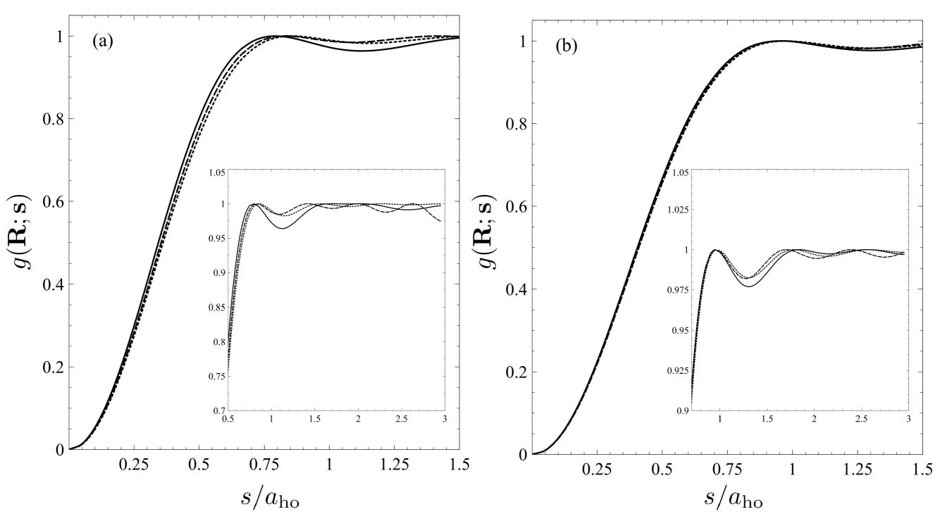
Figure 1: Solid, dashed and dotted curves correspond to the radial distribution functions, $g^{\rm ex}(R;s)$, $g^{\rm sc}(R;s)$ and $g^{\rm LDA}(R;s)$, respectively. Panel (a) is evaluated for $R=0$, and panel (b) is for $R=\frac{1}{2}R_{\rm TF}$, where the Thomas-Fermi radius is given by $R_{\rm TF}/a_{\rm ho}=\sqrt{2\sqrt{2N}}$ with $N=55$ particles. As defined by Eq. (37), $g({\bf R};{\bf s})$ is dimensionless. The insets to both panels depict a zoomed-in, extended range for the radial distribution functions. The axes of the insets are as in the main figure.

IV Summary

We have applied the semiclassical $\hbar$-expansion of Grammaticos and Voros to construct a manifestly Hermitian, idempotent, one-body density matrix for a two-dimensional Fermi gas to second-order in $\hbar$. While our density matrix also satisfies the consistency criterion of the Euler equation, it does not remedy the fact that in two-dimensions, the noninteracting kinetic energy functional has vanishing gradient corrections to all orders in $\hbar$.

As an interesting application, we have provided a detailed calculation for the second-order correction to the Hartree-Fock energy of a spin-polarized, two-dimensional dipolar Fermi gas. We find a small, but finite, negative gradient correction to the local-density approximation. To test the quality of the correction, we have performed numerical comparisons with the known exact results for a harmonically confined, spin-polarized, two-dimensional Fermi gas. We find that including the gradient correction yields superlative agreement with the exact dipole-dipole interaction energy, at least for the case of harmonic confinement.

There are several areas of research where the results of this paper may be useful. One could use our beyond local-density approximation for the total dipole-dipole interaction energy in a density-functional theory application for the equilibrium, collective properties, and density instabilities, of a spin-polarized two-dimensional dipolar Fermi gas. We also see potential applications of our one-body density matrix for developing gradient corrected interaction energy density functionals in inhomogeneous, two-dimensional degenerate electronic systems, which could be used in, e.g., density-functional theory studies of two-dimensional quantum dots. Finally, it would be of interest to consider our semiclassical expansion to higher order in $\hbar$, so that we may ascertain if such corrections remain finite, and if so, to determine whether the semiclassical expansion is convergent or asymptotic.

Appendix A

In the following we shall evaluate Eq. (22).

$$A = \frac{g}{(2\pi\hbar)^{2}}\int_{0}^{p_{F}}dp~{}p\int_{0}^{2\pi}d\phi~{}e^{ips\cos(\phi)/\hbar}$$ (51)

$$= \frac{g}{2\pi s^{2}}\int_{0}^{z}du~{}uJ_{0}(u)~{},$$

where we have put $u=ps/\hbar$ and $z=k_{F}s$. The resulting integral can be performed using Mathematica^© and, gives

$$A=g\frac{k_{F}^{2}}{2\pi}\frac{J_{1}(z)}{z}$$ (52)

Appendix B

The evaluation of Eq. (23) proceeds as follows.

$$B = \frac{g}{(2\pi\hbar)^{2}}\frac{\hbar^{2}}{8m}\nabla^{2}_{\bf R}V\int_{0}^{\infty}dp~{}p\delta^{\prime}(H_{\rm cl}-E_{F})\int_{0}^{2\pi}d\phi~{}e^{ips\cos(\phi)/\hbar}$$ (53)

$$= g\frac{2\pi}{(2\pi\hbar)^{2}}\frac{\hbar^{2}}{8m}\nabla^{2}_{\bf R}V\int_{0}^{\infty}dp~{}p\delta^{\prime}(H_{\rm cl}-E_{F})J_{0}\left(\frac{ps}{\hbar}\right)~{}.$$

Using Eq. (27), we can write

$$B = g\frac{m}{16\pi p_{F}}\nabla^{2}_{\bf R}V\int_{0}^{\infty}dp~{}\frac{d\delta(p-p_{F})}{dp}J_{0}\left(\frac{ps}{\hbar}\right)$$ (54)

$$= g\frac{m}{16\pi\hbar^{2}k_{F}^{2}}\nabla^{2}_{\bf R}V({\bf R})zJ_{1}(z)~{},$$

where we have used $\frac{dJ_{0}(x)}{dx}=-J_{1}(x)$. Finally, we may use $\nabla^{2}_{\bf R}V({\bf R})=-\frac{\hbar^{2}}{2m}\nabla_{\bf R}^{2}k_{F}^{2}$ to write

$$B=-g\frac{1}{32\pi}\frac{\nabla_{\bf R}^{2}k_{F}^{2}}{k_{F}^{2}}~{}zJ_{1}(z)~{}.$$ (55)

Appendix C

The evaluation of Eq. (24) may be performed if we write

$$C = g\frac{1}{48\pi m}(\nabla^{2}_{\bf R}V)^{2}\int_{0}^{\infty}dp~{}p\delta^{\prime\prime}(H_{\rm cl}-E_{F})J_{0}\left(\frac{ps}{\hbar}\right)~{}.$$ (56)

Upons substituting Eq. (28), we obtain

$$C = g\frac{m^{2}}{48\pi p_{F}}(\nabla^{2}_{\bf R}V)^{2}\int_{0}^{\infty}dp~{}\left[\frac{1}{p}\frac{d^{2}\delta(p-p_{F})}{dp^{2}}-\frac{1}{p^{2}}\frac{d\delta(p-p_{F}}{dp}\right]J_{0}\left(\frac{ps}{\hbar}\right)$$ (57)

$$= g\frac{m^{2}}{48\pi p_{F}}(\nabla^{2}_{\bf R}V)^{2}\left\{\frac{d^{2}}{dp^{2}}\left[\frac{1}{p}J_{0}\left(\frac{ps}{\hbar}\right)\right]+\frac{d}{dp}\left[\frac{1}{p^{2}}J_{0}\left(\frac{ps}{\hbar}\right)\right]\right\}_{p=p_{F}}~{}.$$

Recalling that $z=p_{F}s/\hbar=k_{F}s$, we can write

$$C = g\frac{m^{2}}{48\pi p_{F}}(\nabla^{2}_{\bf R}V)^{2}\frac{s^{3}}{\hbar^{3}}\left\{\frac{d^{2}}{du^{2}}\left[\frac{J_{0}(u)}{u}\right]+\frac{d}{du}\left[\frac{J_{0}(u)}{u^{2}}\right]\right\}_{u=z}$$ (58)

$$= g\frac{m^{2}}{48\pi\hbar^{4}k_{F}^{4}}(\nabla_{\bf R}V)^{2}z^{3}\left\{\frac{d^{2}}{dz^{2}}\left[\frac{J_{0}(z)}{z}\right]+\frac{d}{dz}\left[\frac{J_{0}(z)}{z^{2}}\right]\right\}~{}.$$

Performing the derivatives with respect to $z$ gives after simplification (we have used Mathematica^©),

$$\frac{d^{2}}{dz^{2}}\left[\frac{J_{0}(u)}{z}\right]+\frac{d}{dz}\left[\frac{J_{0}(z)}{z^{2}}\right]=\frac{J_{2}(z)}{z}~{}.$$ (59)

Substituting Eq. (59) into Eq. (58), we get

$$C = g\frac{m^{2}}{48\pi\hbar^{4}k_{F}^{4}}(\nabla_{\bf R}V)^{2}z^{2}J_{2}(z)$$ (60)

$$= g\frac{1}{192\pi}z^{2}J_{2}(z)\frac{(\nabla_{\bf R}k_{F}^{2})^{2}}{k_{F}^{4}}~{},$$

where in going to the last line in Eq. (60), we have made use of $\nabla_{\bf R}V=-\frac{\hbar^{2}}{2m}(\nabla_{\bf R}k_{F}^{2})$.

Appendix D

Equation (25) is the most difficult to evaluate, and requires some care. Let us first rewrite Eq. (25) in the following form

$$D = \frac{g}{(2\pi\hbar)^{2}}\frac{\hbar^{2}}{24m^{2}}\sum_{i=1}^{2}\sum_{j=1}^{2}\left[\frac{\partial^{2}V}{\partial X_{i}\partial X_{j}}\right]\int d^{2}p~{}p_{i}p_{j}e^{i{\bf p}\cdot{\bf s}/\hbar}\delta^{\prime\prime}(H_{\rm cl}-E_{F})~{}.$$ (61)

Next, we make use of the identity

$$p_{i}p_{j}e^{i{\bf p}\cdot{\bf s}/\hbar}=-\hbar^{2}\frac{\partial^{2}e^{i{\bf p}\cdot{\bf s}/\hbar}}{\partial s_{i}\partial s_{j}}~{},$$ (62)

which allows us to write

$$D = -g\frac{\hbar^{2}}{96\pi^{2}m^{2}}\sum_{i=1}^{2}\sum_{j=1}^{2}\left[\frac{\partial^{2}V}{\partial X_{i}\partial X_{j}}\frac{\partial^{2}}{\partial s_{i}\partial s_{j}}\right]\int d^{2}p~{}e^{i{\bf p}\cdot{\bf s}/\hbar}\delta^{\prime\prime}(H_{\rm cl}-E_{F})$$ (63)

$$= -g\frac{\hbar^{2}}{48\pi m^{2}}\sum_{i=1}^{2}\sum_{j=1}^{2}\left[\frac{\partial^{2}V}{\partial X_{i}\partial X_{j}}\frac{\partial^{2}}{\partial s_{i}\partial s_{j}}\right]\int_{0}^{\infty}dp~{}p~{}\delta^{\prime\prime}(H_{\rm cl}-E_{F})J_{0}\left(\frac{ps}{\hbar}\right)$$

$$= -g\frac{\hbar^{2}m}{48\pi p_{F}}\sum_{i=1}^{2}\sum_{j=1}^{2}\left[\frac{\partial^{2}V}{\partial X_{i}\partial X_{j}}\frac{\partial^{2}}{\partial s_{i}\partial s_{j}}\right]\int_{0}^{\infty}dp~{}\left[\frac{1}{p}\frac{d^{2}\delta(p-p_{F})}{dp^{2}}-\frac{1}{p^{2}}\frac{d\delta(p-p_{F}}{dp}\right]J_{0}\left(\frac{ps}{\hbar}\right)~{},$$

and proceeding as we did for the evaluation of $C$, we arrive at

$$D = -g\frac{m}{48\pi\hbar^{2}k_{F}^{4}}\sum_{i=1}^{2}\sum_{j=1}^{2}\left[\frac{\partial^{2}V}{\partial X_{i}\partial X_{j}}\frac{\partial^{2}}{\partial s_{i}\partial s_{j}}\right]z^{2}J_{2}(z)~{}.$$ (64)

Let us now define

$$U\equiv\frac{\partial^{2}}{\partial s_{i}\partial s_{j}}(z^{2}J_{2}(z))~{}.$$ (65)

Once again, using $z=p_{F}s/\hbar$, we obtain

$$U = \frac{p_{F}}{\hbar}\frac{\partial}{\partial s_{i}}\left[\frac{s_{j}}{s}\frac{\partial(z^{2}J_{2}(z))}{\partial z}\right]$$ (66)

$$= \frac{p_{F}}{\hbar}\left[\frac{\delta_{ij}}{s}\frac{\partial(z^{2}J_{2})}{\partial z}-\frac{s_{i}s_{i}}{s^{3}}\frac{\partial(z^{2}J_{2})}{\partial z}+\frac{s_{j}}{s}\frac{\partial^{2}(z^{2}J_{2})}{\partial z^{2}}\frac{\partial z}{\partial s_{i}}\right]$$

$$= \frac{p_{F}}{\hbar}\left[\frac{\delta_{ij}}{s}\frac{\partial(z^{2}J_{2})}{\partial z}-\frac{s_{i}s_{i}}{s^{3}}\frac{\partial(z^{2}J_{2})}{\partial z}+\frac{p_{F}}{\hbar}\frac{s_{i}s_{j}}{s^{2}}\frac{\partial^{2}(z^{2}J_{2})}{\partial z^{2}}\right]~{}.$$

Finally, making use of the readily derived identity

$$\frac{\partial^{2}(z^{2}J_{2})}{\partial z^{2}}=zJ_{1}(z)+z^{2}J_{0}(z)~{},$$ (67)

we obtain after some straightforward simplification

$$U=k_{F}^{2}\left[\delta_{ij}zJ_{1}(z)+\frac{s_{i}s_{j}}{s^{2}}z^{2}J_{0}(z)\right]~{}.$$ (68)

Using our expression for $U$, Eq. (68), in Eq. (64), we finally arrive at

$$D = -g\frac{m}{48\pi\hbar^{2}k_{F}^{2}}\sum_{i=1}^{2}\sum_{j=1}^{2}\frac{\partial^{2}V}{\partial X_{i}\partial X_{j}}\left[\delta_{ij}zJ_{1}(z)+\frac{s_{i}s_{j}}{s^{2}}z^{2}J_{0}(z)\right]$$ (69)

$$= -g\frac{m}{48\pi\hbar^{2}k_{F}^{2}}\sum_{i=1}^{2}\sum_{j=1}^{2}\frac{\partial^{2}V}{\partial X_{i}\partial X_{j}}\delta_{ij}zJ_{1}(z)-g\frac{m}{48\pi\hbar^{2}k_{F}^{2}}\sum_{i=1}^{2}\sum_{j=1}^{2}\frac{\partial^{2}V}{\partial X_{i}\partial X_{j}}\left[\frac{s_{i}s_{j}}{s^{2}}z^{2}J_{0}(z)\right]$$

$$= -g\frac{m}{48\pi\hbar^{2}k_{F}^{2}}(\nabla^{2}_{\bf R}V)zJ_{1}(z)-g\frac{m}{48\pi\hbar^{2}k_{F}^{2}}\left[\nabla_{\bf R}\left(\nabla_{\bf R}V\cdot\frac{{\bf s}}{s}\right)\cdot\frac{{\bf s}}{s}\right]z^{2}J_{0}(z)$$

$$= g\frac{1}{96\pi}\frac{\nabla^{2}_{\bf R}k_{F}^{2}}{k_{F}^{2}}zJ_{1}(z)+g\frac{1}{96\pi}\frac{z^{2}J_{0}(z)}{k_{F}^{2}}\left[\nabla_{\bf R}\left(\nabla_{\bf R}k_{F}^{2}\cdot\frac{{\bf s}}{s}\right)\cdot\frac{{\bf s}}{s}\right]~{}.$$

Adding the terms $A+B+C+D$ gives Eq. (29).

Appendix E

We wish to evaluate the following integral,

$$I = \int d^{2}R~{}\int d^{2}s~{}\frac{1}{s^{3}}\frac{zJ_{z}(z)J_{0}(z)}{96\pi^{2}}\left[\nabla_{\bf R}\left(\nabla_{\bf R}k_{F}^{2}\cdot\frac{{\bf s}}{s}\right)\cdot\frac{{\bf s}}{s}\right]~{}.$$ (70)

Let us start by presenting what will prove to be a useful expression,

$$\nabla_{\bf R}=\frac{z}{2k_{F}^{2}}\left(\nabla_{\bf R}k_{F}^{2})\right)\frac{d}{dz}~{},$$ (71)

which along the $i$-th direction reads

$$\frac{\partial}{\partial X_{i}}=\frac{z}{2k_{F}^{2}}\left(\frac{\partial k_{F}^{2}}{\partial X_{i}}\right)\frac{d}{dz}~{}.$$ (72)

Now, we write Eq. (70) as

$$I = \frac{1}{96\pi^{2}}\sum_{i=1}^{2}\sum_{j=1}^{2}\int d^{2}s~{}\frac{s_{i}s_{j}}{s^{5}}\int d^{2}R~{}\left[\frac{\partial^{2}k_{F}^{2}}{\partial X_{i}\partial X_{j}}(zJ_{1}(z)J_{0}(z))\right]$$ (73)

$$= -\frac{1}{96\pi^{2}}\sum_{i=1}^{2}\sum_{j=1}^{2}\int d^{2}s~{}\frac{s_{i}s_{j}}{s^{5}}\int d^{2}R~{}\left[\frac{\partial k_{F}^{2}}{\partial X_{j}}\frac{\partial(zJ_{1}(z)J_{0}(z))}{\partial X_{i}}\right]~{}.$$

Utilizing Eq. (72) in Eq. (73), one obtains

$$I = -\frac{1}{192\pi^{2}}\sum_{i=1}^{2}\sum_{j=1}^{2}\int d^{2}R\frac{1}{k_{F}^{2}}\left[\frac{\partial k_{F}^{2}}{\partial X_{j}}\frac{\partial k_{F}^{2}}{\partial X_{i}}\right]\int_{0}^{\infty}ds~{}\frac{z}{s^{4}}\frac{d}{dz}[(zJ_{1}(z)J_{0}(z))]\int_{0}^{2\pi}d\phi~{}s_{i}s_{j}$$ (74)

$$= -\frac{1}{192\pi}\int d^{2}R~{}\frac{(\nabla_{\bf R}k_{F}^{2})^{2}}{k_{F}}\int_{0}^{\infty}dz~{}\frac{1}{z}\frac{d}{dz}[(zJ_{1}(z)J_{0}(z))]~{},$$

where we have used

$$\int_{0}^{2\pi}d\phi~{}s_{i}s_{j}=\pi s^{2}\delta_{ij}~{}.$$ (75)

The $z$-integral in Eq. (74) can be computed using Mathematica^©, and evaluates to $2/\pi$, whence we obtain

$$I = -\frac{1}{96\pi^{2}}\int d^{2}R~{}\frac{(\nabla_{\bf R}k_{F}^{2})^{2}}{k_{F}}$$ (76)

$$= -\frac{1}{12\sqrt{\pi}}\int d^{2}R~{}[\rho({\bf R})]^{5/2}\frac{(\nabla_{\bf R}\rho)^{2}}{\rho^{3}}~{}.$$

Upon taking into account the $-\mu_{0}d^{2}/8\pi$ factor in Eq. (45), we finally arrive at

$$I_{4} = -\frac{\mu_{0}d^{2}}{8\pi}I=\mu_{0}d^{2}\frac{\sqrt{\pi}}{2}\int d^{2}R~{}[\rho({\bf R})]^{5/2}\left(\frac{1}{48\pi^{2}}\frac{(\nabla_{\bf R}\rho)^{2}}{\rho^{3}}\right)~{}.$$ (77)

References

- (1) R. M. Dreizler and E. K.U. Gross, Density Functional Theory: An Approach to the Quantum Many-Body Problem (Springer-Verlag, Berlin, 1990).
- (2) M. Brack and R. K. Bhaduri, Semiclassical Physics, Frontiers in Physics vol 96 , (Westview Press, Bolder, CO, USA, 2003).
- (3) B. P. van Zyl, Phys. Rev. A 68, 033601 (2003).
- (4) I. S. Gradshteyn and I. M. Ryzhik, Table of Integrals, Series, and Products, 7th ed. (Academic, New York, 2007).
- (5) J. Bardeen, Phys. Rev. 49, 653 (1936).
- (6) R. K. Bhaduri and D. W. L. Sprung, Nucl. Phys. A297, 365 (1978).
- (7) I. A. Howard, N. H March and L. M. Nieto, J. Phys. A: Math. Gen. 35, 4895 (2002).
- (8) B. Grammaticos and A. Voros, Ann. Phys. (N.Y.) 123, 359 (1979).
- (9) K. Bencheikh and E. Räsänen, J. Phys. A: Math. Theor. 49, 015205 (2016).
- (10) Note that another common convention in the literature is to write and , in which case the sign of the second term in Eq. (18) becomes positive. Identical results are, of course, obtained for the ODM regardless of the notational convention.
- (11) We have confirmed that by applying the Wigner-Kirkwood (WK) formalism, one obtains an identical -expansion for the ODM. However, in the WK approach, the starting point is the Wigner transform of the one-body Bloch density matrix (sometimes called the propagator), which can be related back to the ODM via an inverse Laplace transform, and yields the ODM in terms of and . See Ref. brack_bhaduri , Ch. 4.
- (12) In the Kirzhnits approach, the ODM is expressed, from the beginning, using and . In this sense, the Kirzhnits ODM does not display the same explicit symmetry as the GV approach, which is formulated in terms of and . We have shown (to be presented in a future publication) that the Kirzhnits ODM is identical to the GV ODM upon an appropriate symmetrization procedure.
- (13) A. Putaja, E. Räsänen, R. Van Leeuwen, J. G. Vilhena, and M. A. L. Marques, Phys. Rev. B 85, 165101 (2012).
- (14) D. A. Kirzhnits, Sov. Phys. JEPT 5, 64 (19570; D. A. Kirzhnits, Field Theoretical Methods in Many-Body Systems (London: Pergamon Press, 1967).
- (15) L. Salasnich, J. Phys. A: Math. Theor. 40, 9987 (2007).
- (16) M. Koivisto and M. J. Stott, Phys. Rev. B 76, 195103 (2007).
- (17) B. P. van Zyl, A. Farrell, E. Zaremba, J. Towers, P. Pisarski, Phys Rev. A 89, 022503 (2014).
- (18) E. K. U. Gross and C. R. Proetto, J. Chem. Theory Comput. 5, 844 (2009).
- (19) B. P. van Zyl, E. Zaremba and P. Pisarski, Phys. Rev. A 87, 043614 (2013).
- (20) M. Brack and B. P. van Zyl, Phys. Rev. Lett. 86, 1574 (2001).