Topologically Protected Loop Flows in High Voltage AC Power Grids

Abstract

Geographical features such as mountain ranges or big lakes and inland seas often result in large closed loops in high voltage AC power grids. Sizable circulating power flows have been recorded around such loops, which take up transmission line capacity and dissipate but do not deliver electric power. Power flows in high voltage AC transmission grids are dominantly governed by voltage angle differences between connected buses, much in the same way as Josephson currents depend on phase differences between tunnel-coupled superconductors. From this previously overlooked similarity we argue here that circulating power flows in AC power grids are analogous to supercurrents flowing in superconducting rings and in rings of Josephson junctions. We investigate how circulating power flows can be created and how they behave in the presence of ohmic dissipation. We show how changing operating conditions may generate them, how significantly more power is ohmically dissipated in their presence and how they are topologically protected, even in the presence of dissipation, so that they persist when operating conditions are returned to their original values. We identify three mechanisms for creating circulating power flows, (i) by loss of stability of the equilibrium state carrying no circulating loop flow, (ii) by tripping of a line traversing a large loop in the network and (iii) by reclosing a loop that tripped or was open earlier. Because voltage angles are uniquely defined, circulating power flows can take on only discrete values, much in the same way as circulation around vortices is quantized in superfluids.

I Introduction

Power grids are networks of electrical lines whose purpose is to deliver electric power from producers to consumers. The ensuing power flows do not usually follow specified paths, instead they divide among all possible paths following Kirchhoff’s laws. Circulating loop flows around closed, geographically constrained loops have been observed in the North American high voltage power grid, sometimes reaching as much as 1GW Casazza (1998); Lerner (2003), delivering no power but dissipating it ohmically. To try and prevent them, grid operators have issued new market regulations and recommended integrating phase angle regulating transformers into the grid Whitley (2008). The network conditions under which circulating power flows emerge, why they are so robust, how much power they dissipate and whether specific network topologies, if any, could prevent them in the first place are issues of paramount importance which have not been addressed to date. At a conceptual level, the definition of circulating loop flows is furthermore ambiguous, being arbitrarily based on an ill-defined separation of power flows into direct, parallel-path and circulating loop flows. Our goal in this manuscript is to understand better the nature of these circulating power flows.

A deep and unexpected analogy between high voltage electric power transmission and macroscopic quantum states such as superfluids and superconductors has been overlooked so far. The operational state of an AC power grid is determined by the complex voltage at each bus, $V_{l}=|V_{l}|\exp[i\theta_{l}]$ which must be single-valued. Summing over voltage angle differences around any loop in the network must therefore give an integer multiple of $2\pi$. This defines topological winding numbers $q_{\alpha}$,

$$q_{\alpha} = \left(2\pi\right)^{-1}\sum_{l=1}^{n_{\alpha}}|\theta_{l+1}-\theta_{l}|\,\in\,\mathbb{Z}\,,$$ (1)

where the sum runs over all $n_{\alpha}$ nodes around any (the $\alpha^{\rm th}$) loop in the network, $|\theta_{l+1}-\theta_{l}|$ gives the angle difference along the $l^{\rm th}$ line in this loop, counted modulo $2\pi$, and node indices are taken modulo $n_{\alpha}$, i.e. $n_{\alpha}+1\rightarrow 1$. The topological meaning of $q_{\alpha}$ is obvious, as it counts the number of times the complex voltage winds around the origin in the complex plane as one goes around the $\alpha^{\rm th}$ loop. The condition $q_{\alpha}\in\mathbb{Z}$ is the same as the condition that leads to quantization of circulation around superfluid vortices Onsager (1949); Feynman (1955) or to flux quantization through a superconducting ring Byers and Yang (1961).

The analogy with superconductivity is complete under the lossless line approximation, where AC transmission lines are assumed purely susceptive (see Supplemental Material) Bergen and Vittal (2000). Then, the active power flowing between two nodes $l$ and $m$ is given by $P_{lm}=B_{lm}|V_{l}||V_{m}|\sin(\theta_{l}-\theta_{m})$, with the elements $B_{lm}$ of the susceptance matrix. This is the DC Josephson current that would flow between two superconductors with phases $\theta_{l}$ and $\theta_{m}$, coupled by a short tunnel junction of transparency $T_{lm}=\hbar B_{lm}|V_{l}||V_{m}|/8e$ Josephson (1962). It has been shown within the lossless line approximation that, in complex networks, various solutions to the power flow problem exist, which differ only by circulating loop currents Dörfler et al. (2013); Delabays et al. (2016). Neglecting ohmic dissipation, it is therefore expected, and has been reported in simple networks Delabays et al. (2016); Taylor (2012); Mehta et al. (2015), that AC power grids may carry circulating loop flows. Topological winding numbers, Eq. (1), lead to the discretization of circulating loop flows, much in the same way as superfluid circulation is quantized around a vortex Onsager (1949); Feynman (1955). Therefore we refer to circulating loop flows as vortex flows from now on. The existence of integer winding numbers has the important consequence that the vortex flows are topologically protected, much in the same way as persistent currents in superconducting loops Tinkham (1975). The integer $q_{\alpha}$ in Eq. (1) measures the number of times the complex voltage $V_{l}=|V_{l}|\exp[i\theta_{l}]$ rotates in the complex plane as one goes around a loop in the network. Changing a vortex flow requires to change the number $q_{\alpha}$ of such rotations, i.e. to untwist $V_{l}$, which cannot be done smoothly without driving $|V_{l}|\rightarrow 0$ somewhere. It is thus hard to get rid of a vortex flow without topological changes in operating electrical networks.

AC power grids however differ from superfluids and superconducting systems in at least two significant ways in that (i) whereas vortices are generated by external magnetic fields (in a superconductor) or sample rotation (in a superfluid), how to create vortex flows in AC power grids is not quite understood, and (ii) superfluids and superconductors are nondissipative quantum fluids, whereas AC power lines dissipate ohmically part of the power they transmit. The lossless line approximation is in fact only partially justified in very high voltage AC power grids, where lines have a conductance that is at least ten times smaller than their susceptance Bergen and Vittal (2000). Still, ohmic losses typically reach 5–10 % of the total transported power. It is therefore important to find out whether the above analogy between high voltage AC power grids and macroscopic quantum states is at all physically relevant. The two main purposes of this manuscript are therefore (i) to investigate how vortex flows can be created in electric power grids and (ii) to investigate how resilient they are to the presence of ohmic dissipation. Our investigations of creation mechanisms amplify on the work of Janssens and Kamagate Janssens and Kamagate (2003) who succinctly discussed one of the three mechanisms we identify below. Investigating basins of stability for different solutions via the Lyapunov function allows us furthermore to shed analytical light on the line reclosing mechanism they proposed Janssens and Kamagate (2003) and give precise bounds on when vortex flows are created in this way. We furthermore find that vortex flows are resilient to reasonable amounts of ohmic dissipation typical of high voltage power grids and that vortex-carrying operating states ohmically dissipate significantly more electric power than vortex-free states.

Loop flows in electric power grids have been investigated before in a number of theoretical and numerical works. We list some of the most important published works we know about. Korsak investigated a simple network where different, linearly stable solutions exist that differ by some circulating loop current Korsak (1972). Tavora and Smith related the existence of different stable fixed points of the power flow problem to the presence of integer winding numbers Tavora and Smith (1972), reflecting the $2\pi$-periodicity of the complex voltage around any loop in the network and its single-valuedness. The characterization of circulating loop flows with topological winding numbers has been pushed further by Janssens and Kamagate Janssens and Kamagate (2003), who also investigated how to generate such loop flows and found one of the three creation mechanisms we discuss below. More recently, Refs. Dörfler et al. (2013); Delabays et al. (2016) showed that within the lossless line approximation, different power flow solutions must be related to one another by circulating loop flows.

While vortex flows and the analogy we just pointed out between macroscopic quantum states and high voltage AC power grids are intellectually interesting in their own right, we stress that they are physically and technically relevant. Circulating loop flows in the GW range have been observed in power grids Casazza (1998); Lerner (2003), which delivered no power but consumed it ohmically. Furthemore it can be expected that with the changes in operational conditions of the power grid brought about by the energy transition – substituting delocalized productions with smaller primary power reserve for large power plants – such circulating loop flows may occur more frequently. We stress, however, that, while power flow solutions are similar to vortex-carrying quantum mechanical states, there is no quantumness in the power flow problem and that high voltage AC power grids are not superconducting.

The paper is organized as follows. In Section II we argue that different solutions to the power flow problem in meshed networks are related to one another via vortex flows. Sections III, IV and V next discuss sequentially the three mechanisms we identified for generating vortex flows. Section V in particular investigates vortex flow creation via reclosing of a line from a basin of attraction point of view, which allows to quantitatively understand how vortex flows are born. Section VI makes the case that vortex flows are robust against the relatively modest amount of ohmic dissipation present in high voltage power networks. Having gained much understanding of vortex flows in simple models in these early Sections, we next discuss vortex creation with and without dissipation on a complex network with the topology of the UK grid. This is done in Section VII. Conclusions and future perspectives are briefly discussed in Section VIII.

II Circulating Loop Flows in Meshed Networks

We start with the lossless line approximation and neglect voltage variations, $|V_{l}|=V_{0}$, $\forall l$. Active power flows are then governed by the following set of equations (see Supplemental Material)

$$P_{l} = \sum_{m}\tilde{B}_{lm}\sin(\theta_{l}-\theta_{m})\,.$$ (2)

Here, $P_{l}$ is the active power injected ($P_{l}>0$) or consumed ($P_{l}<0$) at node $l$, $\theta_{l}$ is the complex voltage angle and $\tilde{B}_{lm}=B_{lm}V_{0}^{2}$. At this level, one has an exact balance between production and consumption, $\sum_{l}P_{l}=0$. The theorem of Refs. Dörfler et al. (2013); Delabays et al. (2016) states that different solutions to Eq. (S2a) on a meshed network differ only by circulating flows around loops in the network. We go beyond the lossless line approximation to see how much validity this theorem keeps in the presence of ohmic losses. Being interested in high voltage grids we neglect voltage fluctuations all through this manuscript, as they correspond to few percents of the rated voltage $V_{0}$. Ohmic losses are introduced by rewriting Eq. (S2a) as

$$P_{l} = \sum_{m}\left(\tilde{B}_{lm}\sin(\theta_{l}-\theta_{m})+\tilde{G}_{lm}[1-\cos(\theta_{l}-\theta_{m})]\right)\,,$$ (3)

where $\tilde{G}_{lm}=G_{lm}V_{0}^{2}$ with elements $G_{lm}$ of the conductance matrix. Because of ohmic dissipation, total production now exceeds total consumption,

$$\Delta P=\sum_{l}P_{l} = \sum_{l,m}\tilde{G}_{lm}\,\left[1-\cos(\theta_{l}-\theta_{m})\right]>0\,.$$ (4)

Eq. (S3) implies in particular that different solutions to Eq. (3) dissipate different amounts $\Delta P$ of active power and therefore require different power injections $\{P_{l}\}\rightarrow\{P_{l}+\delta P_{l}\}$ to compensate for ohmic losses. The set $\{\delta P_{l}\}$ is not uniquely defined, nevertheless, choices exist for which the theorem of Refs. Dörfler et al. (2013); Delabays et al. (2016) remains valid (see Supplemental Material). This is in agreement with Baillieul and Byrnes Bailleul and Byrnes (1982) who stated that ”models for lossless power networks provide valuable insight and understanding for systems with small transfer conductances” and further suggests that circulating loop flows are robust against a moderate amount of ohmic dissipation. Below we numerically confirm this conjecture. Earlier works however suggested that the number of solutions decreases at fixed susceptance when the conductance increases Skar (1980); Bailleul and Byrnes (1982), so that it is expected that circulating loop flows are eventually suppressed when the conductance exceeds some network-dependent threshold.

Focusing next on the operational conditions under which circulating power flows occur, we find three different mechanisms for creating them, (i) by loss of stability of the solution carrying no circulating loop flow, (ii) by tripping of a line traversing a large loop in the network and (iii) by reclosing a loop that tripped or was open earlier Janssens and Kamagate (2003); Coletta and Jacquod (2016). We discuss these three mechanisms sequentially, first without ohmic dissipation.

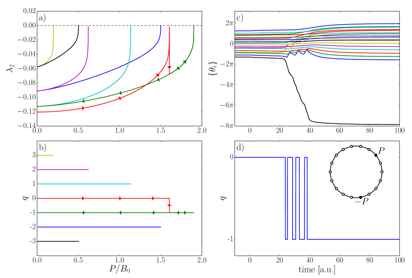
Figure 1: Vortex formation for a ring with $n=18$ nodes. Locations of the main power injection and consumption are indicated by the black nodes in the inset of panel d), while all white nodes have small random injections and consumptions summing to zero, to make the model not too specific (see Supplemental Material). Panels a) and b): stability diagram for solutions with different winding numbers $q$, showing a) the Lyapunov exponent $\lambda_{2}$ and b) the range of stability of the solution. Each spike with $\lambda_{2}\rightarrow 0$ in panel a) indicates the loss of stability of a solution. The red arrows in a) and b) indicate jumps from the $q=0$ solution to that with $q=-1$ as $P$ increases. The path is not retraced, however, as one reverses $P$ back to $P=0$ (green arrows). Panels c) and d): dynamical phase slip as $P/B_{0}=1.575\rightarrow 1.65$ at $t=0$. The $q=0$ solution loses its stability and Eq. (S11) induces a transient behavior where the angle on the consumption site rotates until one reaches the $q=-1$ solution.

III Creating Vortex Flows via Dynamical Phase Slip

Consider first a single-ring, lossless network as illustrated in Fig. 1d. The power flow around the ring is governed by Eq. (S2a) with $\tilde{B}_{lm}=B_{0}$. From Ref. Delabays et al. (2016), the system carries at most nine solutions differing by loop flows, when $B_{0}\rightarrow\infty$. Fig. 1b shows seven of these solutions, each characterized by a winding number $q=-3,-2,...3$. The stability of each solution is determined by the swing equations Bergen and Vittal (2000), which govern the dynamics of the voltage angles $\theta_{l}$ under changes in operating conditions. In this work we neglect inertia terms in swing equations, since their presence affects neither the nature of the stationary states, nor at which parameter values they become unstable Manik et al. (2014); Coletta and Jacquod (2016). In a frame rotating at the grid frequency of 50 or 60 Hz, the swing equations read (see Supplemental Material) Bergen and Hill (1981); Pai (1989); Bergen and Vittal (2000); Backhaus and Chertkov (2013)

$$\dot{\theta_{l}}=P_{l}-\sum_{m=1}^{n}B_{0}\,\sin(\theta_{l}-\theta_{m})\,,\qquad l=1,\ldots n\,.$$ (5)

Stationary solutions to Eq. (S11) are obviously solutions to Eq. (S2a) and their linear stability depends on the stability matrix $M$ obtained after linearizing Eq. (S11) (see Supplemental Material) Pecora and Carroll (1998). A solution of Eq. (S2a) is stable if $M$ is negative semidefinite. We therefore study the stability of each solution via the largest nonvanishing eigenvalue $\lambda_{2}$ of $M$. Fig. 1a shows, together with Fig. 1b how solutions disappear as they lose their stability, $\lambda_{2}\rightarrow 0$. The solution with $q=0$ has the smallest $\lambda_{2}$ at small $P$. Remarkably enough, the $q=0$ solution loses its stability at $P/B_{0}\approx 1.6$, before the $q=-1$ solution, which remains stable until $P/B_{0}\approx 1.85$. Starting from the $q=0$ solution and increasing $P$ beyond 1.6$B_{0}$, we observe a loss of stability followed by a short transient after which the operating state has been transferred to the $q=-1$ state. This transient is illustrated in Fig. 1c and d, which show that mostly one voltage angle, corresponding to the consumer node rotates while all other angles move very little (a movie of this transient can be found in the Supplemental Material). The rotation of this angle changes $q$ which oscillates between $q=0$ and $q=-1$, eventually stabilizing at $q=-1$.

Reducing next $P$ starting from the $q=-1$ solution at $P/B_{0}>1.6$, one remains on the $q=-1$ solution. This hysteretic behavior is indicated by arrows in Fig. 1a and b and illustrates the topological protection brought about by the integer winding number $q$. We have found that this behavior is generic for single-ring networks (see Supplemental Material). The process by which the winding number changes is similar to quantum phase slips in small rings of Josephson junctions Matveev et al. (2002). To emphasize this similarity, while stressing the different physical ingredients at work, we call dynamical phase slip this first mechanism of creation of circulating loop flows.

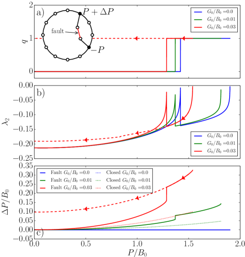
Figure 2: Vortex formation by line tripping in a double loop network with $n=14$ nodes and constant line susceptance $B_{0}$. Locations of the main power injection and consumption are indicated by the black nodes in the inset of panel a), while all white nodes have small random injections and consumptions summing to zero, to make the model not too specific. The initial state corresponds to a $q=0$ state of the double-loop system. The line indicated in red in the inset of panel a) is then tripped, generating a transient to a new operating state. Panels a) and b) show the winding number and the Lyapunov exponent of the new stationary state, for the lossless case (blue line) and for dissipative cases with conductances equal to $1\%$ (green line) and $3\%$ (red line) of the susceptance. The ohmic losses incurred before (dotted lines) and after (solid lines) line tripping are compared in panel c). Arrows on all panels indicate that once created, a vortex flow does not disappear when reducing $P/B_{0}$.

IV The Line Tripping Mechanism

We next investigate the second mechanism for vortex flow generation, by tripping of a line. High voltage AC power grids have a meshed structure, where multiple paths connect production and consumption centers. This ensures that a single line failure does not preclude the supply of electric power. Consider the model shown in the inset of Fig. 2a, where a producer is connected to a consumer via three different paths. Assume then that a line on the middle path trips. The power initially transmitted via that path is redistributed and if $P$ is relatively large, the angle differences $\Delta_{\rm L,R}$ on each remaining path increase significantly. When one of these two paths, say the left one, goes through many more lines than the other one, $N_{\rm L}\gg N_{\rm R}$, it is then possible that $N_{\rm L}\Delta_{\rm L}-N_{\rm R}\Delta_{\rm R}=2\pi q$ with $q>0$, even if the system carried no vorticity initially. This simple example shows how one line tripping in an asymmetrical double-loop system can generate a vortex flow.

Fig. 2 illustrates how a $q\neq 0$ state emerges from a $q=0$ state after a line tripping. The initial state is a stationary state of the double-loop system with zero winding number on both loops. The red line in the inset of Fig. 2a is then cut, which induces a transient driving the system to a stationary state of the resulting single-loop system. Fig. 2a shows the obtained winding number. One sees that for small $P$, the final state has $q=0$, while for larger $P$, a $q=1$ state is reached. We have found that this behavior is generic of sufficiently asymmetric double-loop systems. We discuss cases with ohmic dissipation below.

One may wonder what is the fate of the $q=1$ state created by line tripping when the line is reclosed. Line reclosing is a topological change that has the potential to induce integer changes in the winding number $q$ so that a vortex-free state with $q=0$ can be expected after line reclosing. We show in Fig. 3 that in the present case, line reclosing does not change the winding number and that the vortex flow persists, and that the winding number remains the same, $q=1$. Inspecting the angles in the final state, we find that the vortex in the final state is supported by the larger, left loop.

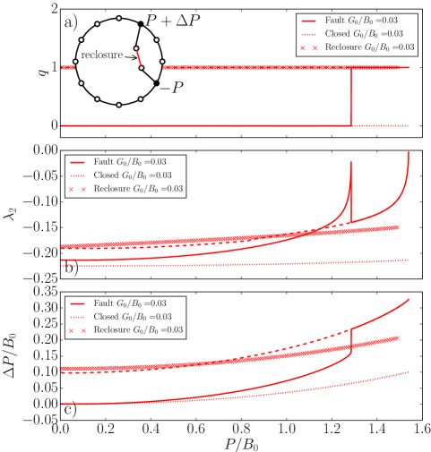
Figure 3: Resilience to line reclosing of the vortex flow created by the line tripping mechanism in Fig. 2. The solid and dashed red lines are the same as in Fig. 2 and correspond to a conductance equal to $3\%$ of the susceptance. The initial state before reclosing is prepared by line tripping at $P/B_{0}=1.55$, followed by reduction of $P/B_{0}$ (arrows in Fig. 2). It has $q=1$ and lies on the dashed red line. The crosses indicate the state obtained after line reclosing at a given value of $P/B_{0}$. The vortex flow survives line reclosing and is located in the larger, left loop.

V Emergence of Vortex Flows from Line Reclosing

We have just showed that line tripping can lead to a vortex flow that is robust against the reclosing of the tripped line. In this paragraph, we finally consider vortex flow creation via reclosing of a line. We consider again the single-loop model sketched in the inset of Fig. 1d. We consider here the case with only one consumer and one producer with some produced (consumed) power $P$ ($-P$) but checked that our conclusions remain the same and that vortex formation proceeds similarly in more complicated single-loop models (see Supplemental Material). We start from the closed-loop system with an operating state with $q=0$. The power $P$ is transferred from producer to consumer both clockwise (via the right path) and counterclockwise (left). One line along the right path then trips, which forces $P$ to be transmitted exclusively along the left path. The voltage angle difference $\Delta_{\rm L}$ between any two nodes along the left path increases, while angle differences along the right path vanish, $\Delta_{\rm R}=0$. This gives an angle difference $\Delta_{0}=N_{\rm L}\Delta_{\rm L}$ between the two nodes on each side of the tripped line. Upon reclosing that line, a current flows through it whose initial direction depends on $\Delta_{0}$, but which eventually relaxes following a dynamical process determined by Eq. (S11). The creation of a vortex flow can however be understood without investigating the voltage angle dynamics, by instead adopting an approach based on the Lyapunov function Pai (1989); Bergen and Vittal (2000). The latter determines the basin of attraction, in voltage-angle space, for the various solutions to the power flow problem Wiley et al. (2006); Menck et al. (2013). The Lyapunov function corresponding to Eq. (S11) reads van Hemmen and Wreskinski (1993)

$${\cal V}(\{\theta_{i}\}) = -\sum_{l}P_{l}\theta_{l}-\sum_{\langle l,m\rangle}B_{0}\,\cos(\theta_{l}-\theta_{m})\,,$$ (6)

where the second sum runs over connected nodes only. Minima of ${\cal V}$ have $\nabla_{\theta}{\cal V}=0$, and thus correspond to stationary power flow solutions. The Lyapunov function can be rewritten as a function of angle differences $\Delta_{l}\coloneqq\theta_{l}-\theta_{l+1}\in[-\pi,\pi]$ as

$$\mathcal{V}(\{\Delta_{i}\}) =-\sum_{l}P_{l}^{*}\Delta_{l}-\sum_{l}B_{0}\cos(\Delta_{l})\,,$$ (7)

where $P_{l}^{*}\coloneqq\sum_{j=1}^{l}P_{j}$, for $l=1,...,n$. The single-loop model we consider here can be split in two paths (left and right) from producer to consumer. We have

$$P_{l}^{*} =\left\{\begin{array}[]{cl}P&\text{if the line from }l\text{ to }l+1\text{ is on the left path,}\\ 0&\text{if the line from }l\text{ to }l+1\text{ is on the right path.}\end{array}\right.$$ (10)

Furthermore, any solution of the nondissipative power flow equations has the same angle differences, $\Delta_{\rm L}=\theta_{l}-\theta_{l+1}$, along each line on the left path and $\Delta_{\rm R}=\theta_{l+1}-\theta_{l}$ on the right path.

Going around the loop, the voltage phases must be well defined. Therefore, just before line reclosing the phase difference $\Delta_{0}$ between the two ends of the tripped line can be written as a function of $\Delta_{\rm L}$ and $\Delta_{\rm R}$, $\Delta_{0}=N_{\rm L}\Delta_{\rm L}-(N_{\rm R}-1)\Delta_{\rm R}-2\pi q$, where $N_{\rm L}>N_{\rm R}\geq 2$ are the number of edges on the left and right paths. Then we can project the Lyapunov function on the $(\Delta_{\rm L},\Delta_{\rm R})$-plane,

$${\cal V}(\Delta_{\rm L},\Delta_{\rm R}) =-N_{\rm L}P\Delta_{\rm L}-N_{\rm L}B_{0}\cos\Delta_{\rm L}-(N_{\rm R}-1)B_{0}\cos\Delta_{\rm R}-B_{0}\cos(N_{\rm L}\Delta_{\rm L}-(N_{\rm R}-1)\Delta_{\rm R})\,.$$ (11)

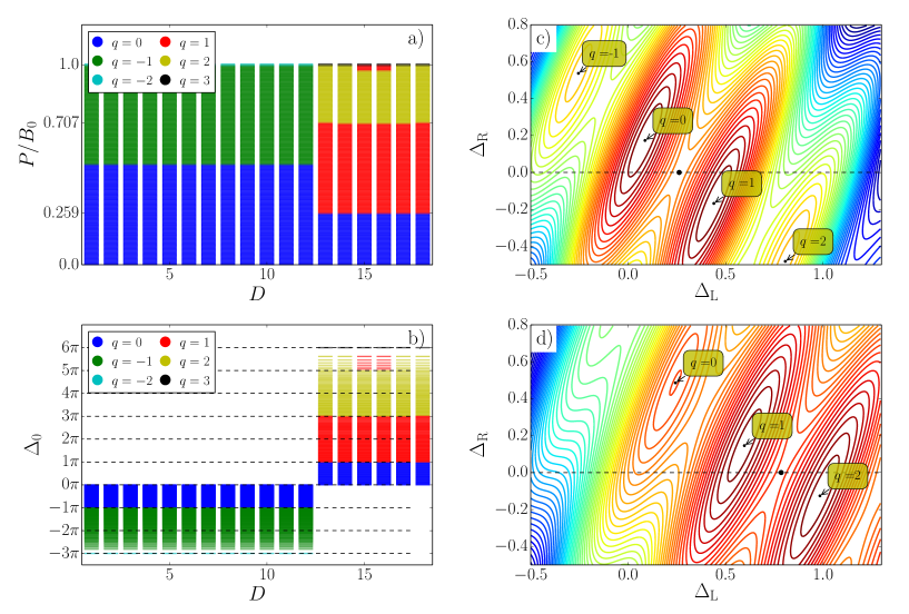
Figure 4: Vortex generation and basins of stability for the single-loop model shown in the inset of Fig. 1d under the line tripping and reclosing mechanism. Panels a) and b): final winding numbers as a function of the position of the tripped line and a) the rescaled injected power $P/B_{0}$, b) the corresponding angle differences $\Delta_{0}$ between the two ends of the tripped line. Panels c) and d): Contour plots of the Lyapunov function for a tripped line at $13\leq D\leq 18$ (on the right path), c) $P=B_{0}\sin(\pi/12)$ and d) $P=B_{0}\sin(\pi/4)$. Local minima with different values of $q$ are indicated. When the line is tripped, $\Delta_{\rm R}=0$ and $\Delta_{0}=12\Delta_{\rm L}$, and black dots show the operating states right before reclosing of the tripped line. For the chosen values of $P/B_{0}$ they are located precisely on saddle points at the boundary between the basins of attraction of $q=0$ and $q=1$ [panel c)], and $q=1$ and $q=2$ [panel d)].

Fig. 4c and d show contour plots of ${\cal V}(\Delta_{\rm L},\Delta_{\rm R})$. Local minima are indicated, together with the corresponding integer winding numbers. To each minimum corresponds a basin of attraction containing the set of initial states that converge towards that minimum under Eq. (S11). All points around a minimum belong to that basin, until one reaches a saddle point or a ridge, beyond which points belong to another basin of attraction. Cutting the right path projects $\Delta_{\rm R}\rightarrow 0$. Right before line reclosing, the system is at $\Delta_{\rm L}=\arcsin(P/B_{0})$ on the dashed lines in Fig. 4c and d which correspond to $P/B_{0}=0.259$ and $P/B_{0}=0.707$ respectively. The solution towards which the system converges after line reclosing depends on the basin of attraction to which the initial state belongs. For $P$ such that $N_{\rm L}\Delta_{\rm L}=\Delta_{0}=(2p+1)\pi$ with $p\in\mathbb{Z}$, the point $(\Delta_{L},\Delta_{\rm R})=(\arcsin(P/B_{0}),0)$ lies right on a saddle-point at the boundary between two basins of attraction, as we now proceed to show.

The gradient of the Lyapunov function $\mathcal{V}$ in the $(\Delta_{\rm L},\Delta_{\rm R})$-plane is given by

$$\nabla\mathcal{V} =\begin{pmatrix}-N_{\rm L}P+N_{\rm L}B_{0}\sin\Delta_{\rm L}+N_{\rm L}B_{0}\sin\left(N_{\rm L}\Delta_{\rm L}-(N_{\rm R}-1)\Delta_{\rm R}\right)\\ (N_{\rm R}-1)B_{0}\sin\Delta_{\rm R}-(N_{\rm R}-1)B_{0}\sin\left(N_{\rm L}\Delta_{\rm L}-(N_{\rm R}-1)\Delta_{\rm R}\right)\end{pmatrix}\,.$$

It is easy to check that $\nabla\mathcal{V}=0$ at $(\Delta_{\rm L},\Delta_{\rm R})=(\arcsin(P/B_{0}),0)$, which is thus a critical point. The nature of this critical point is determined by the two eigenvalues of the Hessian $\mathcal{H}_{\mathcal{V}}$ of $\mathcal{V}$. At our critical point, we obtain

$$\mathcal{H}_{\mathcal{V}}(\arcsin(P/B_{0}),0) =B_{0}\begin{pmatrix}N_{\rm L}\cos\Delta_{\rm L}-N_{\rm L}^{2}&N_{\rm L}(N_{\rm R}-1)\\ N_{\rm L}(N_{\rm R}-1)&(N_{\rm R}-1)-(N_{\rm R}-1)^{2}\end{pmatrix}\eqqcolon\begin{pmatrix}a&b\\ b&c\end{pmatrix}\,.$$

The two eigenvalues of $\mathcal{H}_{\mathcal{V}}$ are then the two roots of

$$\chi(\lambda) =\lambda^{2}-(a+c)\lambda+ac-b^{2}\implies\lambda^{\pm}=\left(a+c\pm\sqrt{(a+c)^{2}-4(ac-b^{2})}\right)/2\,.$$

Then $\lambda^{+}$ is always positive and $\lambda^{-}$ is negative if and only if $ac-b^{2}<0$. Replacing $a$, $b$ and $c$ we have

$$ac-b^{2}=-B_{0}^{2}N_{\rm L}(N_{\rm R}-1)(N_{\rm L}+(N_{\rm R}-2)\cos\Delta_{\rm L})\,,$$ (12)

which is necessarily negative since first, at the moment of the reclosing, $\Delta_{\rm L}=\arcsin(P/B_{0})$ implying that $\cos\Delta_{\rm L}>0$, and second $N_{\rm R}\geq 2$. We conclude that $(\Delta_{\rm L},\Delta_{\rm R})=(\arcsin(P/B_{0}),0)$ for $N_{\rm L}\arcsin(P/B_{0})=(2p+1)\pi$ is a saddle point of the projected Lyapunov function. It can actually be shown that it is a saddle point of the full Lyapunov function. One concludes that vortex generation by this mechanism occurs for $\Delta_{0}>\pi$, and that the final winding number increases by one each time $\Delta_{0}$ crosses an odd integer multiple of $\pi$. The same line of argument with $N_{\rm L}\Delta_{\rm L}\leftrightarrow N_{\rm R}\Delta_{\rm R}$ applies when the line to be cut is on the left path.

The above argument is based on the projected Lyapunov function. It neglects the fact that, after line reclosing, the transient dynamics leaves the $(\Delta_{\rm L},\Delta_{\rm R})$-plane until a new stationary state is reached. We therefore check its validity numerically. Fig. 4 show what final winding number is obtained upon line reclosing depending on the location $D=1,\dots,n$ of the open line (counted counterclockwise, starting from the main producer) and the rescaled power $P/B_{0}$ (Fig. 4a) and $\Delta_{0}$ (Fig. 4b). Fig. 4b confirms that the final winding number changes by one each time $\Delta_{0}$ crosses an odd integer multiple of $\pi$, except when the injected power gets close to its maximal allowed value, $P\rightarrow B_{0}$. We attribute this change of behavior to a more complicated transient in this case. Fig. 4a and b further show that $\Delta_{0}\approx 2\pi$ around $P/B_{0}\approx 0.5$. Taken modulo $2\pi$, this means that the angle difference at the ends of the tripped line is small so that line reclosing is technically feasible.

Fig. 4c) and d) shed a new light on the work of Araposthatis et al. Araposthatis et al. (1981), who discussed the existence of different power flow solutions in separated stable domains in voltage angle space in simple models. Our method allows to visualize different such domains and in particular to infer the precise location of saddle points separating them. Recent works have advocated a new line of research in dynamical systems including coupled oscillators models Wiley et al. (2006); Menck et al. (2013) and AC power networks Menck et al. (2014), investigating the size of basins of attraction. These works were restricted to numerical statistical studies. Our projective approach allows to visualize basins of attractions and the separatrices in between. Quite remarkably, it allows us to understand quantitatively how vortices emerge and when winding numbers change. In both line tripping and line reclosing mechanisms, vortices are created by a topological change in the network, which twists the voltage angles around a loop. We therefore collectively refer to these two mechanisms as topological phase twist.

VI Vortex Flows and Ohmic Dissipation

We next investigate the persistence of circulating loop flows in the presence of ohmic dissipation. Voltage angle differences between connected nodes in operational states of AC power grids seldomly reach more than few tens of degrees, beyond which the power line’s thermal limit is exceeded. Therefore, the dynamical phase slip mechanism (i) is of little relevance for power grid operation, because it occurs when one angle difference $|\theta_{i}-\theta_{j}|\gtrsim\pi/2$ Delabays et al. (2016). We therefore focus on the topological phase twist mechanisms (ii) and (iii).

The green and red lines in Fig. 2 illustrate how ohmic dissipation affects vortex flow creation by tripping of a line. Because ohmic dissipation requires an excess of production to compensate for losses, power production is $P+\Delta P$, larger than the power demand $P$. One sees that the presence of a finite conductance, $\tilde{G}_{lm}\equiv G_{0}\neq 0$ in Eq. (3), reduces the range in $P/B_{0}$ at which transitions between $q=0$ and $q=1$ occur upon line tripping, but that the overall behavior remains the same as long as $G_{0}/B_{0}$ is not too large. Fig. 2c shows furthermore how much more power is consumed in the presence of vortex flows, with a huge stepwise increase in ohmic losses by almost 50% of the losses $\Delta P$ in the presence of a still moderate conductance $G_{0}/B_{0}=0.03$. Fig. 2 finally shows topological protection by the winding number, where once the vortex has been created, returning the operating conditions to smaller $P$ (as indicated by arrows) does not bring the system back to the vortex-free state. Instead, the operational state remains at $q=1$, with losses well above those for $q=0$.

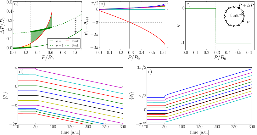
Figure 5: Vortex generation under the line tripping and reclosing mechanism in the presence of ohmic dissipation with $G_{0}/B_{0}=0.05$ for the model shown in the inset of panel c). Panel a): Ohmic losses $\Delta P$ on the closed system with $q=0$ (solid green line) and $q=1$ (dashed green line) and on the open loop with one tripped line (red solid line). We start from the $q=0$ solution and cut the line indicated in the inset of panel c). Upon closing the line again, the system goes from the red line solution to the $q=0$ solution in the yellow area, but jumps to $q=1$ in the green area. The red line stops at $P/B_{0}\approx 0.62$ above which there is no single-path stable solution. Panel b): angle differences before line reclosing. The jump to $q=1$ occurs when the angle difference between the two ends of the tripped line exceeds $\pi$, in complete agreement with the basin of attraction argument, even with dissipation. Panel c): final winding number after the tripped line has been reclosed. Panels d) and e) show topological protection and robust synchrony with modified frequency as $\Delta P$ is changed as indicated by the vertical arrow in panel a) at $P/B_{0}=1$. Panel d): $\Delta P$ is decreased to $\Delta P_{q=0}$ starting from the $q=1$ state, and e) $\Delta P$ is increased to $\Delta P_{q=1}$ from the $q=0$ state, in both cases at $t=50$. Despite the presence of dissipation and the change in $\Delta P$, the winding number is topologically protected.

Fig. 5 makes it clear that vortex generation under the line tripping and reclosing mechanism (iii) proceeds in the same way in the presence of ohmic dissipation. We start from a $q=0$ stationary state, cut a line and let the system relax to a stationary state, after which we close the line again. What final state is obtained depends on $P/B_{0}$. When $P$ is small, the system relaxes back to the initial state with $q=0$ (yellow area in Fig. 5a), however at larger $P$, the transient dynamically moves the system towards the $q=1$ stationary state (green area in Fig. 5a). Fig. 5b shows that the transition to $q=1$ occurs precisely when the voltage angle difference between the nodes surrounding the faulted line reaches $\pi$, even in the presence of ohmic dissipation, in complete agreement with the basin of attraction theory discussed above. We finally note that line reclosing is technically feasible around $P/B_{0}\approx 0.5$ where the angle difference between the two ends of the tripped line is small (modulo $2\pi$). This would lead to a $q=1$ vortex flow state.

Dissipation renders operational conditions different for different stationary states. In particular, states with vortex flows generically have larger ohmic losses, because they have larger angle differences in Eq. (S3). They therefore require an additional power injection $\Delta P_{q}$ depending on the vorticity $q$. One would think that changing the operational conditions by e.g. reducing $\Delta P_{q\neq 0}\rightarrow\Delta P_{q=0}$ makes the $q$-vortex flow disappear. Figs. 5d and e show however that topological protection by the winding number remains active, despite the presence of dissipation. In panel d) we decrease the additional power injection $\Delta P$ to the amount of losses incurred in the $q=0$ stationary state when the system is in the $q=1$ state, while in panel e) we increase $\Delta P$ to its value in the $q=1$ state, starting from the $q=0$ state, at $P/B_{0}=1$. In both cases, the winding number remains the same. Synchronization is furthermore not destroyed, however angles rotate at a modified frequency, $\theta_{i}(t)=\theta_{i}^{(0)}\pm\delta\Omega t$ in the rotating frame, with $\delta\Omega\simeq N^{-1}(\Delta P_{q=1}-\Delta P_{q=0})$. Adapting $\Delta P$ to what is required by another $q$-state changes the synchronous frequency but leaves $q$ unchanged.

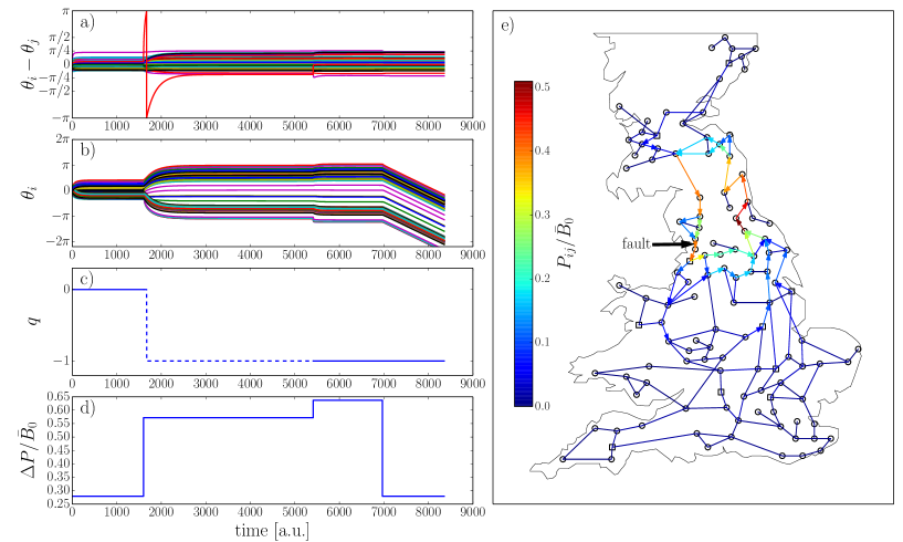
Figure 6: Vortex creation in a complex network with the topology of the UK transmission grid under the line tripping and reclosing mechanism. The grid is sketched in panel e). Lines have capacities inversely proportional to their length and are normalized to $\langle B_{lm}\rangle=\overline{B}_{0}$. There are 10 power generators (indicated by squares ) with $P_{\rm G}=0.5\overline{B}_{0}+\Delta P/10$ and 110 consumers (circles) with $P_{\rm C}=-\overline{B}_{0}/22$. Ohmic dissipation is due to a finite conductance with $G_{lm}/B_{lm}=0.1$, typical of very high voltage AC power lines. Panels a)–d): angle differences, angles, winding number $q$ and ohmic losses as a function of time. We first let the state dynamically converge to a stationary synchronous state without vortex flow. One line then trips at $t=1600$ and the system converges to a new synchronous state with increased ohmic losses. The line is reclosed at $t=5410$ and a vortex flow has been created in the resulting synchronous state, with $q=-1$, increasing ohmic losses further. The additional power injected into the grid to compensate for the ohmic losses is then brought back to its initial value at $t=6970$. The vortex flow persists, angle differences essentially remain unchanged while angles start to rotate in unison, $\theta_{i}=\delta\Omega t$, $\forall i$, indicating a change in synchronous frequency by $\delta\Omega$. The dashed line in panel c) indicate that $q$ is not defined for $t\in[120,330]$, when the loop is open. Panel e): color-coded difference in flows between the initial, $q=0$ stationary state and the final, $q=-1$ state, in units of $B_{lm}$. Arrows indicate the direction of the flow difference only when the latter exceeds 0.05 $\overline{B}_{0}$.

VII Vortex Flows in Complex Grids

We finally export the knowledge obtained from investigating simple systems to a network model with the topology of the UK high-voltage AC power grid Coletta and Jacquod (2016); Witthaut and Timme (2012). Fig. 6 illustrates vortex flow creation, enhanced ohmic losses and topological protection of stationary states with vortex flows. The system is initially stabilized in a stationary state without vorticity on any of its loops. It is later perturbed by a line tripping, at the position indicated in Fig. 6e. The state is then left to stabilize towards a new state, after which it is again perturbed by the reclosing of the line. Finally, the power injected is modified to try and move the system back to the stationary state with $q=0$ – without success. Fig. 6a and b show the behavior of the voltage angles and angle differences between connected nodes. It is seen that line tripping at $t=1600$ essentially makes a single voltage angle difference significantly change, similarly to the single-loop model considered in Fig. 5. The same angle difference is the only one to move sensibly upon line reclosing at $t=5410$. Fig. 6c shows that the line fault creates a vortex flow. The latter is affected by adapting the power at $t=6970$ to the losses of the initial state with $q=0$ only insofar as all its angles start to rotate at a modified frequency $\delta\Omega\simeq N^{-1}(\Delta P_{q=0}-\Delta P_{q=-1})$. However this does not affect its winding number – topological protection is at work also in this case of a complex meshed grid with significant ohmic dissipation, $G_{lm}/B_{lm}=0.1$. Fig. 6d shows that the vortex flow doubles ohmic losses, despite the fact that it affects only a small fraction of the grid, as is seen in Fig. 6e which shows differences in flows between the $q=-1$ and $q=0$ states. The reduction in losses in Fig. 6d after $t=6970$ leads to the synchronization of the grid at a frequency different from the rated frequency of 50 Hz. Such a change in frequency would be intolerable in a real power grid, and would quickly lead to either controlled or uncontrolled line trippings, cascades of failures, possibly leading to blackouts Lehmann and Bernasconi (2010); Vaiman et al. (2012); Pahwa et al. (2014).

VIII Conclusions

Out of the three mechanisms for creating vortex flows we discussed, the topological phase twist mechanisms (ii) and (iii) are relevant to AC power grid operation as they can occur at relatively small voltage angle differences between connected nodes. The reliability of AC power grids is constantly evaluated via $N-1$ feasibility and transient stability analysis, where the existence of a stationary solution as well as the convergence towards that solution is checked after any one of the $N$ major components (lines, transformers etc.) is removed from the network. We believe that this analysis should be complemented by checks of the presence of vortex flows, since the tripping or the reclosing of a line has the potential to generate them, resulting in reduced stability and higher, persistent ohmic losses, that are very difficult to get rid of.

The operating conditions of power grids are expected to change drastically as the energy transition steadily substitutes smaller, delocalized production for large power plants. As but one consequence, power generators have less and less mechanical inertia, thus less primary power reserve. To compensate for these changes, power electronics devices, phase angle regulating transformers and other devices whose task it is to effectively modify admittances and voltage phase angles are often incorporated into the power grid. The two topological phase twist mechanisms discussed above are in a way extreme, in that they rely on line tripping or reclosing. The conditions under which less stringent actions such as reducing line admittances would generate vortex flows should be investigated. Work along those lines is in progress and preliminary results seem to indicate that changes in power grids brought about by the energy transition have the potential to generate vortex flows more frequently.

We also discussed vortex flow creation via dynamical phase slip, despite its lack of relevance for AC power grids. High voltage power transmission is however closely connected to problems of coupled oscillators via the celebrated Kuramoto model Kuramoto (1984); Strogatz (2000); Acebrón et al. (2005); Arenas et al. (2008). Connections between the latter model and Josephson junction arrays were noted in Ref. Wiesenfeld et al. (1998). Stationary states in systems of coupled oscillators with different winding numbers were discussed in Ref. Rogge and Aeyels (2004); Ochab and Góra (2010) and in a biological context in Ref. Heitmann and Ermentrout (2015). Our theory can be exported to those situations to explain how such states are created in the first place and how they disappear.

We finally comment on further analogies with vortex physics in superconductors. First, the point has already been made above that there is no counterpart to external magnetic fields in electrical grids that could generate vortices, and at present it is not known to us whether specific sequences of injection/consumption changes could lead to the creation of vortex flows. But if such a sequence exists, Fig. 4 shows that it should move the system over an ”energy” barrier, i.e. over a ridge or a saddle point of the Lyapunov function. This, in a sense, is to be related to vortex formation in the Ginzburg-Landau model for type II superconductors where an energy barrier is passed at a critical magnetic field beyond which the vortex state is energetically favorable. Second, vortex creation in superfluids occurs either via creation of a pair of vortex-antivortex or via vortex nucleation at the boundary of the system. Electrical power grids being rather small, we have found that vortex nucleation occurs at the network boundary, but would need to perform numerically intensive investigations on much bigger networks (the North American or the Pan-European networks for instance) to see if/when vortex-antivortex pairs are created. While we cannot rule out single vortex creation in the bulk from topological line modifications such as line tripping or reclosing, we suspect this occurs only very rarely, if at all, as such a process would require winding numbers to change simultaneously for a macroscopic number of loops encircling the vortex. Finally, it is known that vortices in superconductors move in the presence of a transport current, which leads to dissipation. So far we have seen vortex flows move only in numerical investigations on regular lattices. That we never saw it in complex networks may be due to either the finiteness of the system size considered, or to the absence of large loops neighboring those where vortex flows sit or to vortex pinning in these complex, effectively disordered networks. With our current knowledge, whether vortex flows can move around in large electric power grids is an open question.

Topologically Protected Loop flows in High Voltage AC Power Grids: Supplemental Material

S1 The power flow problem

Power grids are AC electrical networks. Mathematically speaking, they are modeled as graphs with $n$ nodes, each of them representing a bus and the graph’s edges representing electrical lines.

The standard operating state of electric power grids is characterized by synchrony, where voltage angles on all buses rotate at the same frequency. That state is reached and maintained thanks to the coupling between buses induced by power lines and a balance regulation between power production and consumption, which forbid voltage angles from deviating from a predetermined frequency by more than a fraction of a percent. Production and consumption are constantly fluctuating and accordingly the synchronous state of the system constantly changes. Most of the time, however, these changes are so slow that the whole system is effectively in a steady-state determined by one of the solutions to the power flow equations,

$$P_{l} = \sum_{m}B_{lm}\,|V_{l}||V_{m}|\,\sin(\theta_{l}-\theta_{m})+G_{lm}\left[|V_{l}|^{2}-|V_{l}||V_{m}|\cos(\theta_{l}-\theta_{m})\right]\,,$$ (S1a)

$$Q_{l} = \sum_{m}B_{lm}\,\left[|V_{l}|^{2}-|V_{l}||V_{m}|\cos(\theta_{l}-\theta_{m})\right]-G_{lm}\,|V_{l}||V_{m}|\,\sin(\theta_{l}-\theta_{m})\,,$$ (S1b)

which we take as our starting point. These are transcendental equations for balanced 3-phase systems Bergen and Vittal (2000), which relate the phase and amplitude of the complex AC voltage $V_{m}=|V_{m}|\exp[i\theta_{m}]$ at the bus connecting the $m^{\rm th}$ component (a producer or a consumer) to the grid, to the active, $P_{l}$, and reactive, $Q_{l}$, powers injected ($P_{l},Q_{l}>0$) or consumed ($P_{l},Q_{l}<0$) at the $l^{\rm th}$ bus via power lines of complex admittance $Y_{lm}=G_{lm}+iB_{lm}$. In its full version, the problem is defined by splitting the $n$ buses into producer and consumer buses with pre-determined $\{P_{l},|V_{l}|\}$ and $\{P_{l},Q_{l}\}$ respectively. With these conditions fixed, Eqs. (S1) then determine angles at all buses, voltages at consumer buses and reactive powers at producer buses.

High voltage power lines typically have a conductance to susceptance ratio $G_{lm}/B_{lm}<0.1$, becoming smaller at higher voltage. A first level of approximation is thus to neglect the conductance and with it all ohmic dissipation and to consider

$$P_{l} = \sum_{m}B_{lm}|V_{l}||V_{m}|\,\sin(\theta_{l}-\theta_{m})\,,$$ (S2a)

$$Q_{l} = \sum_{m}B_{lm}\,\left[|V_{l}|^{2}-|V_{l}||V_{m}|\cos(\theta_{l}-\theta_{m})\right]\,.$$ (S2b)

Eqs. (S2) give the lossless line approximation. At that level, one may consider voltage variations that are necessary to accomodate predetermined amounts of reactive power $Q_{l}$ at consumer nodes. However, a standardly used level of approximation Filatrella et al. (2008); Chopra and Spong (2009); Arenas et al. (2008) is to neglect voltage variations and consider $|V_{l}|=V_{0}$, $\forall l$, to introduce an effective line susceptance $\tilde{B}_{lm}=B_{lm}V_{0}^{2}$, and to focus on the power flow equation for the active power only, Eq. (S2a), since, within that approximation, it decouples from the reactive power. We will follow that approach. Within the lossless line approximation, the analogy between AC power grids and current biased Josephson junction arrays is evident : power flows between buses $l$ and $m$ in AC power grids have the same sinusoidal dependence on voltage angle differences, $\tilde{B}_{lm}\sin(\theta_{l}-\theta_{m})$, that Josephson currents between two tunnel-coupled superconductors have on the phases of the order parameters Josephson (1962).

The fact that the lines are lossless manifests itself in the power balance between production and consumption, $\sum_{l}P_{l}=0$. When the conductance $G_{lm}$ is not negligible, the power dissipated must be compensated by an increased power injection. When dissipation is taken into account, one has

$$\sum_{l}P_{l} = \sum_{l,m}\tilde{G}_{lm}\,\left[1-\cos(\theta_{l}-\theta_{m})\right]\,,$$ (S3)

where we defined $\tilde{G}_{lm}\equiv G_{lm}V_{0}^{2}$. Starting from the lossless perspective and considering dissipative effects as a perturbation, it is evident from Eq. (S3) that different solutions to Eq. (S2a) dissipate different amounts of power. Thus, for the full problem (including dissipation), these different solutions generally require different power injections and the power flow problem is no longer defined a priori by a set of power injections $\{P_{i}\}$ which sum up to zero. Power production must be greater than the consumption to compensate the ohmic losses. Thus power injection must be adapted self-consistently with the angles. In our simulations we will achieve that by increasing/decreasing power injection depending on the frequency of the synchronous solution as obtained from the swing equations, Eq. (S12). This procedure is iterated until the dynamical system converges toward a synchronous stationary solution having the reference frequency. Clearly ohmic losses can be compensated by different injection profiles and this procedure is a priori not uniquely defined. A standard procedure in electrical engineering is to predetermine all but one power injections and consumptions and introduce a slack bus, that injects whatever additional power is needed to balance production with consumption and satisfy Eq. (S3). This is the approach we follow in our simulations on simple network topologies presented hereafter and in the main text. For the simulation of the complex network having the topology of the UK transmission grid (see main text) we assume instead that all producers equally compensate for the ohmic losses.

S2 Number of different power flow solutions

Refs. Dörfler et al. (2013); Delabays et al. (2016) showed that different solutions to the dissipationless power flow Eq. (S2) exist on meshed networks, and that these different solutions are related to one another by circulating loop flows, i.e. power flows going around closed loops formed in the network. We sketch here the proof of that theorem. It is based on the incidence matrix $A$ of the network, whose row indices correspond to nodes (buses) and column indices to the network edges (the links between nodes), and which is defined as

$$A_{li}=\left\{\begin{array}[]{ll}1\,,&\text{if node }l\text{ is the source of edge }i\,,\\ -1&\text{if node }l\text{ is the target of edge }i\,,\\ 0\,,&\text{otherwise}\,.\end{array}\right.$$ (S4)

The dissipationless power flow problem can be rewritten in terms of the incidence matrix as

$$P_{l} =\sum_{i}A_{li}\,I_{i}\,,$$ (S5)

where $I_{i}$ is a component of the vector of flows on the network’s edges. It is easy to see that two solutions of Eq. (S5) differ by a flow vector with components $\delta I_{i}$ satisfying

$$0 =\sum_{i}A_{li}\,\delta I_{i}\,,$$ (S6)

and which therefore belongs to the kernel of the incidence matrix. The proof is completed by invoking a known result of algebraic graph theory that any element in $\ker(A)$ is a linear combination of unitary flows along loops formed in the network Biggs (1993). Reference Delabays et al. (2016) also discusses how these different solutions can be labeled by integer topological winding numbers.

We qualitatively discuss the fate of circulating loop flows in cases with dissipation, i.e. nonegligible conductance. From Eq. (S4), for each element of the incidence matrix $A_{li}\neq 0$ there is exactly one $A_{mi}=-A_{li}$, where $l$ and $m$ label the two ends of edge $i$. Thus contributions from each nondissipative, susceptive flow $I_{i}$ appear for both ends of edge $i$ in Eq. (S5), contributing to $P_{l}$ and $P_{m}$ with opposite sign. This parity antisymmetry is characteristic of nondissipative flows. On the contrary, the dissipative part of the flow is parity symmetric - a current of fixed magnitude on a given edge gives the same dissipation, regardless of the direction in which it traverses the line. Adding dissipation therefore requires to add a resistance matrix $R$ with $R_{li}=|A_{li}|$. Eq. (S5) becomes, in the presence of dissipation

$$P_{l} =\sum_{i}A_{li}\,I_{i}+R_{li}\,J_{i}\,,$$ (S7)

with a dissipated power flow $J_{i}\geq 0$. The difference between two power flow solutions then reads

$$\delta P_{l} =\sum_{i}A_{li}\,\delta I_{i}+R_{li}\,\delta J_{i}\,.$$ (S8)

Summing over all nodes one gets

$$\sum_{l}\delta P_{l} =\sum_{l,i}R_{li}\,\delta J_{i}\,,$$ (S9)

which, similarly as Eq. (S3), says that the net total injected power is solely due to the dissipative part of the power flow. Assuming that the equality in Eq. (S9) holds term by term, one obtains again Eq. (S6) so that the two solutions differ by loop flows only. How this can be achieved in practice is easily seen starting from the lossless line approximation, Eq. (S2), which, as was shown in Refs. Dörfler et al. (2013); Delabays et al. (2016), carries solutions $\{\theta_{i}^{(0)}\}$ differing by loop flows only. Once dissipation is added, these solutions remain valid if one chooses to change the injected and consumed powers as $P_{l}\rightarrow P_{l}+\delta P_{l}$ with

$$\delta P_{l} = \sum_{m}\bar{G}_{lm}\,\left[1-\cos(\theta_{l}^{(0)}-\theta_{m}^{(0)})\right]\,.$$ (S10)

This suggests that, at least for not too strong dissipation, i.e. for weak conductance to susceptance ratios, different solutions to the power flow problem exist. For two such solutions, the transmitted powers still differ by loop flows. Extending the results of Refs. Dörfler et al. (2013); Delabays et al. (2016) is straightforward with the choice of Eq. (S10) for compensating losses, because angles are not modified. In the main text, we numerically use another procedure, where the additional power necessary to counterbalance ohmic losses is injected from a single bus. This is a standard approach in electrical engineering where a slack bus ensures that the total power balance is satisfied Bergen and Vittal (2000).

Because the power flow problem in the presence of dissipation becomes higher-dimensional, with additional degrees of freedom related to the choice of producers in charge of compensating the ohmic dissipation, it is much harder to make general statements about the extension of the theorem of Refs. Dörfler et al. (2013); Delabays et al. (2016) to that case. Nevertheless, from Eq. (S10) it is clear that since solutions indexed by high topological winding numbers (i.e. solutions carrying large loop flows) are characterized by larger phase differences, they will in general lose more power to ohmic losses.

S3 Dynamics and stability

For each producer and consumer bus, energy conservation states that the injected or consumed power is equal to the transmitted power (with a negative or positive sign depending on whether it flows toward or away from the bus considered) minus the losses, including transmission line losses as well as mechanical damping losses. This balance condition leads to the swing equations Bergen and Vittal (2000)

$$M_{l}\ddot{\theta}_{l}+\dot{\theta_{l}}=P_{l}-\sum_{m}\left(B_{lm}\,|V_{l}||V_{m}|\,\sin(\theta_{l}-\theta_{m})+G_{lm}\left[|V_{l}|^{2}-|V_{l}||V_{m}|\cos(\theta_{l}-\theta_{m})\right]\right)\,,$$ (S11)

which we write here in a frame rotating with the frequency $\Omega/2\pi=50$ or 60 Hz of the grid. The terms $M_{l}\ddot{\theta}_{l}$ and $\dot{\theta}_{l}$ in Eq. (S11) represent the change in rotational kinetic energy and the damping of the rotating machines connected to the grid.

In this work we consider a simplified version of the swing equations where the mechanical inertia of generators is neglected, i.e. where instead of Eq. (S11) we consider

$$\dot{\theta_{l}}=P_{l}-\sum_{m}\tilde{B}_{lm}\,\sin(\theta_{l}-\theta_{m})+\tilde{G}_{lm}\left[1-\cos(\theta_{l}-\theta_{m})\right]\,.$$ (S12)

While the inertia term affects stability time scales Bergen and Vittal (2000), it does not influence whether a solution is linearly stable or not, which is our interest here. In particular it can be shown that linear stability is lost for a power grid modeled by Eq. (S12) at the same time it would be lost for the same set of equations extended with inertia terms with any distribution of inertia $\{M_{l}\}$ Coletta and Jacquod (2016); Manik et al. (2014). We therefore neglect inertia terms from now on.

Solutions to the power flow equations, Eq. (S1), are stationary solutions of the swing equations, Eq. (S12). The latter allows to determine the linear stability of power flow solutions $\{\theta_{l}^{(0)}\}$ under small perturbations, $\theta_{l}^{(0)}\rightarrow\theta_{l}^{(0)}+\delta\theta_{l}$. Within the lossless line approximation, the linearized dynamics reads

$$\delta\dot{\theta_{l}}=-\sum_{m}\tilde{B}_{lm}\,\cos(\theta_{l}^{(0)}-\theta_{m}^{(0)})(\delta\theta_{l}-\delta\theta_{m})\,.$$ (S13)

The linear stability of the solution is therefore determined by the spectrum of the stability matrix $M(\{\theta_{l}^{(0)}\})$,

$$M_{lm}=\left\{\begin{array}[]{cl}\tilde{B}_{lm}\cos(\theta_{l}^{(0)}-\theta_{m}^{(0)})&\quad\text{if }l\neq m\,,\\ \displaystyle-\sum_{k\neq l}\tilde{B}_{lk}\cos(\theta_{l}^{(0)}-\theta_{k}^{(0)})&\quad\text{if }l=m\,,\end{array}\right.$$ (S14)

which depends on the angles at the stationary, phase-locked solution. The eigenvalues of $M$ are the so-called Lyapunov exponents Pai (1989). Without dissipation, $M$ is real symmetric, therefore all Lyapunov exponents are real, furthermore one of them always vanishes, $\lambda_{1}=0$, because $\sum_{j}M_{ji}=\sum_{j}M_{ij}=0$. This condition is similar to a gauge invariance according to which only angle differences matter. The stationary state is thus linearly stable if $M$ is negative semidefinite and unstable otherwise. Equivalently, stability is ensured as long as the largest nonvanishing eigenvalue $\lambda_{2}$ of $M$ remains negative.

In the dissipative case, the definition of the stability matrix generalizes to

$$M_{lm}=\left\{\begin{array}[]{cl}\tilde{B}_{lm}\cos(\theta_{l}^{(0)}-\theta_{m}^{(0)})-\bar{G}_{lm}\sin(\theta_{l}^{(0)}-\theta_{m}^{(0)})&\quad\text{if }l\neq m\,,\\ \displaystyle-\sum_{k\neq l}\left(\tilde{B}_{lk}\cos(\theta_{l}^{(0)}-\theta_{k}^{(0)})-\bar{G}_{lk}\sin(\theta_{l}^{(0)}-\theta_{k}^{(0)})\right)&\quad\text{if }l=m\,.\end{array}\right.$$ (S15)

Thus, in the presence of dissipation, the stability matrix maintains its zero row sum property (ensuring that $\lambda_{1}=0$) but is no longer symmetric which can lead to a complex spectrum. In this case linear stability is ensured as long as the real part of all nonvanishing eigenvalues of $M$ is negative. To make contact with the nondissipative case, we denote by $\lambda_{2}$ the eigenvalue having the largest real part.

S4 Dynamical generation of vortices

The first mechanism for generating vortex flows discussed in the main text is based on the loss of stability of power flow solutions with lower winding numbers while solutions with higher winding numbers remain stable. This is done by increasing power generated and consumed, which, depending on the grid’s geometry leads to a line congestion and a temporary dynamical instability, eventually driving the system to a new, stable stationary state with redistributed power flows. The model considered in the main text is a ring of $n=18$ nodes, with one main producer at node 1 and one main consumer at node 7. Small random injections at all other nodes are introduced to remove a mirror symmetry along the axis going through nodes 4 and 13. This symmetry results in $\dot{\theta}_{i}=-\dot{\theta}_{{\cal P}(i)}$ with ${\cal P}(i)$ denoting the mirror symmetric node to $i$. Analytically, this forbids transitions to other $q$-values starting from any stationary $q=0$ states. Numerically it results in very long transients with anomalously long angle rotations. To show that our model is generic and that its behavior is not an artefact of random injections/consumptions we discuss a different model which corroborates our conclusions in the main text.

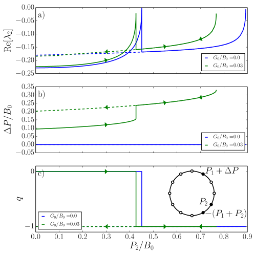
Figure S1: Dynamical generation of vortices by line weakening for a ring with $n=12$ nodes and lines of susceptance $B_{0}$. Locations of the main power injections and consumptions are indicated by the black nodes in the inset of panel c), while all white nodes have small random injections and consumptions summing to zero, to make the model more generic. As the consumer demand is increased from $-P_{1}=-B_{0}$ to $-P_{1}-P_{2}$ units of power, the transmission path connecting the comsumer to its neighboring producer weakens forcing additional power to flow around the other side of the loop. As the power demand is increased beyond $P_{2}\simeq 0.45B_{0}$ for the lossless case, and $P_{2}\simeq 0.42B_{0}$ for the dissipative case $G_{0}/B_{0}=0.03$, the $q=0$ solution becomes unstable [panel a)] driving the system into a state with winding number $q=-1$. This state is highly dissipative and, as indicated by the arrows, it is topologically protected.

In Fig. S1 we illustrate a similar mechanism based on the weakening of a line on a network loop by an additional power injection. We consider a single loop of $n=12$ nodes and lines of capacity $B_{0}$. Initially, a first producer supplies $P_{1}=B_{0}$ units of power to a consumer located four nodes away from it. The transmitted power splits over the two possible paths joining the producer to the consumer. Next, the consumption is increased from $-P_{1}$ to $-P_{1}-P_{2}$. To meet this additional power demand, a second generator, neighboring the consumer, injects a power $P_{2}>0$ (see inset of Fig. S1). This additional power injection increases the load of the line connecting the consumer to the second generator. This weakening of the transmission path eventually drives part of the injection of the first producer away from its original path, around the other side of the loop. Fig. S1 illustrates this mechanism respectively in the lossless and dissipative cases where, for the latter, the first generator is in charge of fully compensating the ohmic losses $\Delta P$. The $q=0$ solution loses stability when the additional power injection reaches $P_{2}\simeq 0.45B_{0}$ (resp. $P_{2}\simeq 0.42B_{0}$ for $G_{0}/B_{0}=0.03$), which drives the system to the $q=-1$ solution. That solution remains stable until $P_{2}\simeq 0.9B_{0}$ (resp. $P_{2}\simeq 0.77B_{0}$ for $G_{0}/B_{0}=0.03$). In the dissipative case, the $q=-1$ solution significantly increases ohmic losses doubling them at $P_{2}=0$. The arrows indicate the hysteretic behavior where decreasing $P_{2}$ from the $q=-1$ solution at $P_{2}\simeq 0.77B_{0}$ does not bring the system back to the $q=0$ solution. This topological protection forces the power system to produce more to compensate for the additional ohmic losses despite the existence of a less dissipative solution. When the system is in the $q=-1$ state for $P_{2}\lesssim 0.42B_{0}$, reducing $\Delta P$ to the value required by the $q=0$ solution drives the system to a $q=-1$ synchronous state with reduced frequency, but not to the $q=0$ state.

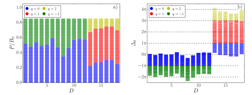
Figure S2: Vortex generation under the line reclosing mechanism, for the single-loop model shown in the inset of Fig. 1d in the main text, with additional random power injection in the intermediate nodes. The final winding numbers, after reclosing, are color-coded and plotted as a function of the position $D$ of the tripped line and a) the rescaled injected power $P/B_{0}$, b) the angle differences $\Delta_{0}$ between the two ends of the tripped line. Vortex generation occurs as soon as $\Delta_{0}\geq\pi$ and higher winding numbers $q$ are reached each time $\Delta_{0}$ crosses an odd integer multiple of $\pi$. This shows that the argument presented in the main text holds even in the more general situation with power injections between the main producer and the main consumer.

S5 Generation of vortices by line reclosing

The line reclosing mechanism discussed in the main text considers a big producer connected to a big consumer on a loop where all other buses have $P_{l}=0$. This allows to project the $(n-1)$-dimensional configuration space of angles on a two-dimensional space and in this way to visualize the basins of attraction of solutions with different winding numbers (Fig. 2c and d of the main text). It was found that the winding numbers change by one each time the angle difference $\Delta_{0}$ between the buses at the two ends of the line to be reclosed crosses an odd integer multiple of $\pi$. These findings are generic, in that they remain valid under the addition of randomly distributed power injections/consumptions on intermediate buses between the big producer and consumer. This is illustrated in Fig. S2. Compared to Fig. 2 of the main text, the presence of random injections/consumptions strongly modifies the borders between reconnected solutions with different $q$ in the $P/B$ vs. $D$ plane (panel a) but not in the $\Delta_{0}$ vs. $D$ plane (panel b). This is so because the small random injections change the value of $P$ necessary for $\Delta_{0}=(2p+1)\pi$. One sees that, despite the presence of random power injections, vortex flows are generated by line reconnection as soon as $|\Delta_{0}|>\pi$, but not earlier, and that the created vortex has a winding number increasing/decreasing as $\Delta q={\rm mod}(\Delta_{0}+\pi,2\pi)$ with good precision. This confirms that the findings presented in the main text are generic and not restricted to the a priori ideal situation considered there.

S6 Basins of attraction and the projected Lyapunov function

In this section we present some details on the basins of attraction of solutions having different winding numbers in the context of the line tripping and reclosing mechanism for the model depicted in the inset of Fig. 1d of the main text.

In the main text, we show that the Lyapunov function projected on the $(\Delta_{\rm L},\Delta_{\rm R})$-plane reads,

$${\cal V}(\Delta_{\rm L},\Delta_{\rm R}) =-N_{\rm L}P\Delta_{\rm L}-N_{\rm L}B_{0}\cos\Delta_{\rm L}-(N_{\rm R}-1)B_{0}\cos\Delta_{\rm R}-B_{0}\cos(\Delta_{0})$$

$$=-N_{\rm L}P\Delta_{\rm L}-N_{\rm L}B_{0}\cos\Delta_{\rm L}-(N_{\rm R}-1)B_{0}\cos\Delta_{\rm R}-B_{0}\cos(N_{\rm L}\Delta_{\rm L}-(N_{\rm R}-1)\Delta_{\rm R})\,.$$ (S16)

This is Eq. (9) in the main text. Also in the main text, we show that the point $(\Delta_{\rm L},\Delta_{\rm R})=(\arcsin(P/B_{0}),0)$ (the system’s state just before reclosing of the faulty line) is a saddle point of the Lyapunov function (S16), if $P$ is such that $N_{\rm L}\Delta_{\rm L}=(2p+1)\pi$ for $p\in\mathbb{Z}$. Inspection of the Hessian of the Lyapunov function allows us further to show that $(\Delta_{\rm L},\Delta_{\rm R})=(\arcsin(P/B_{0}),0)$ for $N_{\rm L}\arcsin(P/B_{0})=(2p+1)\pi$ is a saddle point of the projected Lyapunov function. We can thus tune parameters precisely in such a way that when the line is reclosed, one gets a final operating state with the desired vorticity.

Fig. S3 gives a contour plot of the Lyapunov function for the $18$ node cycle network considered in the main text which illustrates how the final vorticity can be tuned. Depending on the value of the power injected [panels a) to c)], the state of the system at the moment of the line reclosing lies either in the basin of attraction of the $q=0$ solution, or in that of the $q=1$ solution, or at a saddle point separating them.

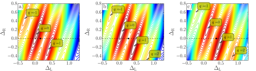
Figure S3: Contour plots of the projected Lyapunov function for the 18 node cycle network described in the main text [see Fig. 1d)] and injected powers $P\approx 0.159B_{0}$ panel a), $P=B_{0}\sin(\pi/12)\approx 0.259B_{0}$ panel b), and $P\approx 0.359B_{0}$ panel c). Local minima at different values of $q$ are indicated. The operating state obtained by tripping one line on the shortest path between the generator and the producer ($\Delta_{\rm R}=0$, $\Delta_{\rm L}=\arcsin{(P/B_{0})}$, and $\Delta_{0}=12\Delta_{\rm L}$) is indicated by the black dot on each panel. It lies in the basin of attraction of the $q=0$ state for $P<0.259B_{0}$ [case a)], in the basin of atttraction of the $q=1$ state for $P>0.259B_{0}$ [case c)], and at the saddle point separating the two basins for $P=0.259B_{0}$ [case b)].

References

- Casazza (1998) J. Casazza, Electrical World 212, 62 (1998).
- Lerner (2003) E. J. Lerner, The Industrial Physicist 9, 8 (2003).
- Whitley (2008) S. G. Whitley, Lake Erie Loop Flow Mitigation (Technical Report; New York Independent System Operator, 2008).
- Onsager (1949) L. Onsager, Nuovo Cimento 6, 249 (1949).
- Feynman (1955) R. P. Feynman, Progress in Low Temperature Physics 1, 34 (1955).
- Byers and Yang (1961) N. Byers and C. N. Yang, Phys. Rev. Lett. 7, 46 (1961).
- Bergen and Vittal (2000) A. R. Bergen and V. Vittal, Power Systems Analysis (Prentice Hall, 2000).
- Josephson (1962) B. D. Josephson, Phys. Lett. 1, 251 (1962).
- Dörfler et al. (2013) F. Dörfler, M. Chertkov, and F. Bullo, Proc. Natl. Acad. Sci. 110, 2005 (2013).
- Delabays et al. (2016) R. Delabays, T. Coletta, and P. Jacquod, J. Math. Phys. 57, 032701 (2016).
- Taylor (2012) R. Taylor, J. Phys. A 45, 055102 (2012).
- Mehta et al. (2015) D. Mehta, N. Daleo, F. Dörfler, and J. D. Hauenstein, Chaos 25 (2015).
- Tinkham (1975) M. Tinkham, Introduction to Superconductivity (Krieger Publishing Company, 1975).
- Janssens and Kamagate (2003) N. Janssens and A. Kamagate, Int. J. Elect. Power Energy Syst. 25, 591 (2003).
- Korsak (1972) A. Korsak, IEEE Trans. Power App. Syst. , 1093 (1972).
- Tavora and Smith (1972) C. J. Tavora and O. J. Smith, IEEE Trans. Power App. Syst. , 1131 (1972).
- Bailleul and Byrnes (1982) J. Bailleul and C. Byrnes, Proc. of the 21st IEEE Conf. on Decision and Control 2, 919 (1982).
- Skar (1980) S. Skar, Stability of Power Systems and other Systems of Second Order Differential Equations, Ph.D. thesis, Iowa State University (1980).
- Coletta and Jacquod (2016) T. Coletta and P. Jacquod, Phys. Rev. E 93, 032222 (2016).
- Manik et al. (2014) D. Manik, D. Witthaut, B. Schäfer, M. Matthiae, A. Sorge, M. Rohden, E. Katifori, and M. Timme, Eur. Phys. J. Special Topics 223, 2527 (2014).
- Bergen and Hill (1981) A. R. Bergen and D. J. Hill, IEEE Trans. Power App. Syst. PAS-100, 25 (1981).
- Pai (1989) M. A. Pai, Energy Function Analysis for Power System Stability (Kluwer Academic Publishers, 1989).
- Backhaus and Chertkov (2013) S. Backhaus and M. Chertkov, Physics Today 66, 42 (2013).
- Pecora and Carroll (1998) L. M. Pecora and T. L. Carroll, Phys. Rev. Lett. 80, 2109 (1998).
- Matveev et al. (2002) K. A. Matveev, A. I. Larkin, and L. I. Glazman, Phys. Rev. Lett. 89, 096802 (2002).
- Wiley et al. (2006) D. A. Wiley, S. H. Strogatz, and M. Girvan, Chaos 16, 015103 (2006).
- Menck et al. (2013) P. J. Menck, J. Heitzig, N. Marwan, and J. Kurths, Nat. Phys. 9, 89 (2013).
- van Hemmen and Wreskinski (1993) J. L. van Hemmen and W. F. Wreskinski, J. Stat. Phys. 72, 145 (1993).
- Araposthatis et al. (1981) A. Araposthatis, S. Sastry, and P. Varayia, Int. J. Elect. Power Energy Syst. 3, 115 (1981).
- Menck et al. (2014) P. J. Menck, J. Heitzig, J. Kurths, and H. J. Schellnhuber, Nat. Comms. 5, 3969 (2014).
- Witthaut and Timme (2012) D. Witthaut and M. Timme, New Journal of Physics 14, 083036 (2012).
- Lehmann and Bernasconi (2010) J. Lehmann and J. Bernasconi, Phys. Rev. E 81, 031129 (2010).
- Vaiman et al. (2012) M. Vaiman, K. Bell, Y. Chen, B. Chowdhury, I. Dobson, P. Hines, M. Papic, S. Miller, and P. Zhang, IEEE Transactions Power Systems 27, 631 (2012).
- Pahwa et al. (2014) S. Pahwa, C. Scoglio, and A. Scala, Sci. Rep. 4, 3694 (2014).
- Kuramoto (1984) Y. Kuramoto, Progr. Theoret. Phys. Suppl. 79, 223 (1984).
- Strogatz (2000) S. Strogatz, Physica D 143, 1 (2000).
- Acebrón et al. (2005) J. Acebrón, L. Bonilla, C. Pérez Vicente, F. Ritort, and R. Spigler, Rev. Mod. Phys. 77, 137 (2005).
- Arenas et al. (2008) A. Arenas, A. Díaz-Guilera, J. Kurths, Y. Moreno, and C. Zhou, Physics Reports 469, 93 (2008).
- Wiesenfeld et al. (1998) K. Wiesenfeld, P. Colet, and S. Strogatz, Phys. Rev. E 57, 1563 (1998).
- Rogge and Aeyels (2004) J. A. Rogge and D. Aeyels, J. Phys. A 37, 11135 (2004).
- Ochab and Góra (2010) J. Ochab and P. F. Góra, Acta Phys. Pol. B [Proc. Suppl. 3] 3, 453 (2010).
- Heitmann and Ermentrout (2015) S. Heitmann and G. B. Ermentrout, Biol. Cybern. 109, 333 (2015).
- Filatrella et al. (2008) G. Filatrella, A. H. Nielsen, and N. F. Pedersen, The European Physical Journal B 61, 485 (2008).
- Chopra and Spong (2009) N. Chopra and M. W. Spong, IEEE Transactions on Automatic Control 54, 353 (2009).
- Biggs (1993) N. Biggs, Algebraic graph theory, 2nd ed. (Cambridge University Press, 1993).