Investigation into spiral phase plate contrast in optical and electron microscopy

Abstract

The use of phase plates in the back focal plane of a microscope is a well established technique in optical microscopy to increase the contrast of weakly interacting samples and is gaining interest in electron microscopy as well. In this paper we study the spiral phase plate (SPP), also called helical, vortex, or two-dimensional Hilbert phase plate, that adds an angularly dependent phase of the form $e^{i\ell\phi_{k}}$ to the exit wave in Fourier space. In the limit of large collection angles, we analytically calculate that the average of a pair of $\ell=\pm 1$ SPP filtered images is directly proportional to the gradient squared of the exit wave, explaining the edge contrast previously seen in optical SPP work. We discuss the difference between a clockwise–anticlockwise pair of SPP filtered images and derive conditions under which the modulus of the wave’s gradient can be seen directly from one SPP filtered image. This work provides the theoretical background to interpret images obtained with a SPP, thereby opening new perspectives for new experiments to study for example magnetic materials in an electron microscope.

I Introduction

Inserting phase plates in the back focal plane of a microscope, whether optical Born and Wolf (1999); Martin (1966); Barer (1953) or electron Danev and Nagayama (2001, 2008); Kaneko et al. (2006), is a well established technique to increase the contrast of transparent objects. This way even pure phase objects can be made visible. In optical microscopy this technique was first developed with the introduction of the Zernike phase plate Zernike (1942a, b) adding a $\pm\pi/2$ phase difference to the scattered part of the wave compared to the transmitted part and was followed by other types of phase-imaging methods including the differential interference contrast (DIC) microscopy Pluta (1994) and Hoffman modulation contrast (HMC) microscopy Hoffman and Gross (1975). In electron microscopy charging and contamination impedes the design of workable phase plates significantly. A first equivalent to the Zernike phase plate, the Boersch phase plate Boersch (1947), adds an extra phase to the scattered wave using a charged metallic ring in the Fourier plane Matsumoto and Tonomura (1996); Schultheiß et al. (2006); Majorovits et al. (2007). An alternative way of imparting a phase shift on the scattered beam is to use a thin film carbon sheet with a hole in the center Danev and Nagayama (2001); Shimada et al. (2007); Yamaguchi et al. (2008). Both techniques have been demonstrated experimentally, but show complications that prevent general application. Only recently a workable electron Zernike phase plate called the Volta phase plate was designed where a thin film is introduced in the back focal plane. The unscattered beam modifies the surface of the film, giving the central beam its phase shift Danev et al. (2014) and has been successfully applied in cryo-tomography Asano et al. (2015); Mahamid et al. (2016) and single particle analysis Khoshouei et al. (2016). Also an electron equivalent to the DIC method has been shown Danev et al. (2002); Kaneko et al. (2005, 2006); Nitta et al. (2009). Depending on the shape of the phase plate, the transparent object is made visible in different ways. Images made with a Zernike phase plate are (to a first-order approximation) direct phase contrast images, where the intensity in the image is proportional to the phase shift of the wave. In images made with the DIC and HMC method, the transparent objects are revealed as if they are illuminated from one side, appearing bright on one side and casting a shadow on the other.

Some particularly interesting types of phase plate are the one- and two-dimensional Hilbert phase plates Davis et al. (2000); Danev et al. (2002). In the one-dimensional case, one side of the wave in Fourier space is given a $\pi$ phase shift with respect to the other. Edges perpendicular to this direction then appear as bright lines in the image. In order to remove the directional dependency of the edge-enhancement, the two-dimensional radially symmetric Hilbert phase plate can be used that adds a phase of the form $\exp(i\ell\phi_{k})$ to the wave in Fourier space, where $\phi_{k}$ is the angular coordinate with respect to the center of the beam and $\ell$ is an integer number. When $\ell=\pm 1$, there is a $\pi$-phase shift across any diameter of the phase plate. Note that these phase plates, called vortex, helical or spiral phase plates (SPP), can also be used to generate vortex beams that are characterized by a wavefunction of the form $\Psi(\bm{r})=\psi(r)e^{i\ell\phi}e^{ik_{z}z}$ Nye and Berry (1974); Allen et al. (1992), which have their own fields of application in optics Galajda and Ormos (2001); Friese et al. (2001); Luo et al. (2000); He et al. (1995); Swartzlander and Hernandez-Aranda (2007); Serabyn et al. (2010); Berkhout and Beijersbergen (2008); Wang et al. (2012); Roychowdhury et al. (2004) and electron microscopy Verbeeck et al. (2013); Juchtmans et al. (2015). In phase-contrast microscopy, these phase plates have been proven to be useful in optics Fürhapter et al. (2005), but also in electron microscopy they are attracting increasingly more attention as an edge–enhancement technique Blackburn and Loudon (2014) or to detect the chirality of crystals Juchtmans and Verbeeck (2015). For charged particles the one-dimensional Hilbert phase shift can be induced using the Aharonov-Bohm phase shift of a thin magnetized wire placed along the diameter of an aperture Nagayama (2008). In a same way, the angularly dependent phase of the two-dimensional Hilbert phase can be generated near the tip of a magnetized needle Béché et al. (2013); Blackburn and Loudon (2014); Béché et al. (2016a). Although alternative SPPs for electrons have been investigated, e.g., fork gratings Verbeeck et al. (2010) or helically shaped lenses made of a transparent material Béché et al. (2016b), the magnetic phase plates have the advantage of only blocking a relatively small part of the aperture in the objective plane, such that a maximal amount of scattered electrons can contribute to the signal.

In previous work Juchtmans and Verbeeck (2016), we related the intensity of images obtained with a SPP to the local OAM decomposition of the exit wave. However, in ref. Davis et al. (2000) it was shown that the same phase plate enhances the contrast at edges of transparent objects in all directions, and in ref. Fürhapter et al. (2005) it was suggested that the intensity in the images is related to the gradient of the exit wave.

In this paper, we analytically investigate what a SPP with $\ell=\pm 1$ reveals about the exit wave and its partial derivatives within the approximation of large collection angles and verify this with numerical simulations. Based on this, we discuss under which circumstances the SPP filtered images can be directly linked to the gradient of the wave, and when this approximation no longer holds. Finally, we shortly discuss how the combined information of three images made with a $\ell=-1$, $\ell=0$ and a $\ell=1$ SPP may provide enough information to make a full exit wave reconstruction of both the phase and intensity.

II Images with $\ell=\pm 1$ spiral phase plates

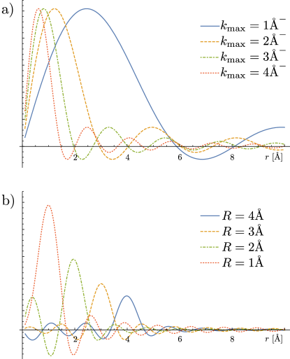
Figure 1: The radial profiles of the FT of flat amplitude SPP apertures with different radii $k_{\text{max}}\in\{1,2,3,4\}\text{\AA}^{-1}$ (a) and for Bessel modulated amplitude SPP apertures with $k_{\text{max}}$=5Å ^- for different $R$ (b)

In the following $\Psi(\bm{r})=\Psi(r,\phi)$ and $\tilde{\Psi}(\bm{k})=\tilde{\Psi}(k,\phi_{k})$ denote a two-dimensional section of the three-dimensional wave in real and Fourier space respectively.

Let $\Psi(\bm{r})$ be a two-dimensional wave of interest, e.g., scalar electromagnetic wave or electron wave after interaction with a sample. Introducing a spiral phase plate (SPP) into the back focal plane of a microscope means that we add a phase of the form $e^{i\ell\phi_{k}}$, with $\phi_{k}$ the angular coordinate and $\ell=\pm 1$ an integer, to the scattered wave in the diffraction plane. Mathematically this means we multiply the Fourier transform (FT) of the exit wave with an angularly dependent phase factor

$$\tilde{\Psi}^{\pm}(\bm{k})=\begin{cases}\tilde{\Psi}(\bm{k})e^{\pm i\phi_{k}}\hskip 28.45274pt&\bm{(}k\neq 0)\\ 0&(k=0),\end{cases}$$ (1)

where we set the amplitude of the wave to zero in the origin since the phase factor $e^{\pm i\phi_{k}}$ is undefined in this point. To obtain the resulting image, we must propagate to real space by taking the inverse Fourier transform

$${\Psi}^{\pm} =\mathcal{F}^{-1}[\tilde{\Psi}(\bm{k}).e^{\pm i\phi_{k}}](\bm{r})$$

$$=\mathcal{F}^{-1}[\tilde{\Psi}(\bm{k})]\otimes\mathcal{F}^{-1}[e^{\pm i\phi_{k}}]$$

$$=\Psi(\bm{r})\otimes\mathcal{F}^{-1}[e^{\pm i\phi_{k}}],$$ (2)

where we used the convolution theorem in the second transformation. The resulting image therefore is given by the convolution of the exit wave with the Fourier transform of the SPP. It is easy to show that the latter has a radially symmetric amplitude with an angularly dependent phase factor $e^{\pm i\phi}$, i.e.,

$$\mathcal{F}^{-1}[e^{\pm i\phi_{k}}]=\int_{0}^{\infty}dk\int_{0}^{2\pi}d\phi_{k}\,ke^{\pm i\phi_{k}}e^{i\bm{k}\cdot\bm{r}}$$

$$=\int_{0}^{\infty}dk\int_{0}^{2\pi}d\phi_{k}\,ke^{\pm i\phi_{k}}\sum_{m}i^{m}J_{m}(kr)e^{im(\phi-\phi_{k})}$$

$$=2\pi\sum_{m}i^{m}e^{im\phi}\int_{0}^{\infty}dk\,kJ_{m}(kr)\delta_{m,\pm 1}$$

$$=2\pi ie^{\pm i\phi}\int_{0}^{\infty}dk\,kJ_{1}(kr),$$ (3)

where we used the Jacobi–Anger identity

$$e^{ikr\cos(\phi-\phi_{k})}=\sum_{m}i^{m}J_{m}(kr)e^{im(\phi-\phi_{k})}.$$ (4)

The above expression for the Fourier transform of the SPP is not normalizable, i.e., is a distribution. In reality however, the upper boundary of the integral in eq. 3 is given by the radius of the SPP aperture ($k_{\text{max}}$)

$$\mathcal{F}^{-1}[\pm SPP] =2\pi ie^{\pm i\phi}\int_{0}^{k_{\text{max}}}dk\,kJ_{1}(kr)$$

$$=T^{k_{\text{max}}}(r)e^{\pm i\phi},$$ (5)

where $T^{k_{\text{max}}}(r)$ is a function that determines the radial profile of the FT of an $\ell=\pm 1$ SPP. The function has a global maximum close to zero, but is zero at $r=0$, which gives the Fourier transform of the SPP the typical vortex beam shape, a bright ring with a dark core. As shown in fig. 1a, the larger the radius of the SPP aperture, $k_{\text{max}}$, the more sharply $T^{k_{\text{max}}}(r)$ is peaked near $r=0$. The radius of this ring is inversely proportional to the size of the phase plate aperture and can be made arbitrarily small when an idealized microscope, aberration corrected at large collection angles, is assumed. We should note here that, although the ring can be made arbitrarily small, it will not converge to an infinitely sharp delta-ring, because tails will always be present. In order to remove these, a SPP that modulates the amplitude of the wave with a first-order Bessel function, $J_{1}(kR)$, can be used Wei et al. (2011); Grillo et al. (2014), where $R$ is a parameter that determines the radius of the ring. In contrast to the constante amplitude (flat) SPP, in the limit of large $k_{\text{max}}$, the profile of the FT of the Bessel amplitude modulated aperture converges to a $\delta$-peak. However, since the Bessel modulated aperture also is not normalizable it needs a cut-off at a certain $k_{\text{max}}$, giving rise to a broadening of the $\delta$-peak, as can be seen in fig. 1b for $k_{\text{max}}$=5 Å^-. In what follows all calculations assume a flat SPP, but can easily be extended for a Bessel amplitude modulated SPP.

Figure 2: Scheme of the wavefunction in polar coordinates at points $\bm{r}$ and $\bm{r}+\bm{dr}$ given by $\Psi(r,\phi)$ and $\Psi(r+dr,\phi+d\phi)$.

Using a flat SPP, the convolution in eq. 2 can be written as

$$\Psi^{\pm} =\int^{\infty}_{0}dr^{\prime}\int^{2\pi}_{0}d{\phi^{\prime}}\,r^{\prime}\Psi(\bm{r}-\bm{r^{\prime}})e^{\pm i\phi^{\prime}}T^{k_{\text{max}}}(r^{\prime}).$$ (6)

As mentioned above, we can choose $k_{\text{max}}$ such that $T^{k_{\text{max}}}(r^{\prime})$ can be made arbitrarily peaked near $r^{\prime}=0$. For a sufficiently large aperture, $\psi$ can thus be approximated by its first order Taylor expansion in the entire region where $T^{k_{\text{max}}}(\bm{r}^{\prime})$ has a significant weight. In polar coordinates, defined in fig. 2, the first order Taylor expansion of $\psi$ reads

$$\Psi(r+\mathrm{d}r,\phi+\mathrm{d}\phi)\approx\Psi(r,\phi)+$$

$$\frac{\partial{\Psi(r,\phi)}}{\partial{r}}r^{\prime}\cos(\phi-\phi^{\prime})+\frac{\partial{\Psi(r,\phi)}}{\partial{\phi}}\frac{r^{\prime}}{r}\sin(\phi-\phi^{\prime}),$$ (7)

and the convolution in eq. 6 becomes

$$\Psi^{\pm} =\int^{\infty}_{0}dr^{\prime}\int^{2\pi}_{0}d{\phi^{\prime}}\,r^{\prime}e^{\pm i\phi^{\prime}}T^{k_{\text{max}}}(r^{\prime})\Big{(}\Psi(r,\phi)+$$

$$\left.\frac{\partial{\Psi(r,\phi)}}{\partial{r}}r^{\prime}\cos(\phi-\phi^{\prime})+\frac{\partial{\Psi(r,\phi)}}{\partial{\phi}}\frac{r^{\prime}}{r}\sin(\phi-\phi^{\prime})\right)$$

$$= \int^{\infty}_{0}dr^{\prime}\,r^{\prime}T^{k_{\text{max}}}(r^{\prime})\times$$

$$\left(0-\frac{\partial{\Psi(r,\phi)}}{\partial{r}}r^{\prime}\pi e^{i\phi}\mp i\frac{\partial{\Psi(r,\phi)}}{\partial{\phi}}\frac{r^{\prime}}{r}\pi e^{i\phi}\right)$$

$$= \left(\frac{\partial{\Psi(r,\phi)}}{\partial{r}}\pm\frac{i}{r}\frac{\partial{\Psi(r,\phi)}}{\partial{\phi}}\right)\pi e^{i(\phi+\pi)}\int dr^{\prime}\,r^{\prime 2}T^{k_{\text{max}}}(r^{\prime}).$$ (8)

The images obtained with an $\ell=+1$ and $\ell=-1$ SPP are given by the modulus squared $\left|\Psi^{\pm}\right|^{2}$

$$I^{+}=$$

$$C\left(\frac{\partial{\Psi}}{\partial{r}}\frac{\partial{\Psi^{*}}}{\partial{r}}-\frac{i}{r}\frac{\partial{\Psi}}{\partial{r}}\frac{\partial{\Psi^{*}}}{\partial{\phi}}+\frac{i}{r}\frac{\partial{\Psi}}{\partial{\phi}}\frac{\partial{\Psi^{*}}}{\partial{r}}+\frac{1}{r^{2}}\frac{\partial{\Psi}}{\partial{\phi}}\frac{\partial{\Psi^{*}}}{\partial{\phi}}\right)$$ (9)

$$I^{-}=$$

$$C\left(\frac{\partial{\Psi}}{\partial{r}}\frac{\partial{\Psi^{*}}}{\partial{r}}+\frac{i}{r}\frac{\partial{\Psi}}{\partial{r}}\frac{\partial{\Psi^{*}}}{\partial{\phi}}-\frac{i}{r}\frac{\partial{\Psi}}{\partial{\phi}}\frac{\partial{\Psi^{*}}}{\partial{r}}+\frac{1}{r^{2}}\frac{\partial{\Psi}}{\partial{\phi}}\frac{\partial{\Psi^{*}}}{\partial{\phi}}\right),$$ (10)

with $C=\left|\pi\int^{\infty}_{0}dr^{\prime}\,r^{\prime 2}T^{k_{\text{max}}}(r^{\prime})\right|^{2}$ a normalization factor. From eq. 9 and eq. 10 we indeed see that, in the limit of large $k_{\text{max}}$, there is a clear relation between the SPP filtered images and the first partial derivative of the exit wave $\Psi$. However, images taken with oppositely handed SPPs, in general, are not equal to each other and therefor can not be both proportional to the gradient of the exit wave as might be expected from the observation of enhanced edge contrast Davis et al. (2000); Fürhapter et al. (2005).

III Average and difference of $\ell=\pm 1$ SPP filtered images

We can, however, measure the gradient of the wave directly by looking at the average of two opposite SPP filtered images

$$\frac{1}{2}\left(I^{+}+I^{-}\right)= C\left(\frac{\partial{\Psi}}{\partial{r}}\frac{\partial{\Psi^{*}}}{\partial{r}}+\frac{1}{r^{2}}\frac{\partial{\Psi}}{\partial{\phi}}\frac{\partial{\Psi^{*}}}{\partial{\phi}}\right)$$

$$= C\left|\bm{\nabla}_{\perp}\Psi\right|^{2},$$ (11)

where $\bm{\nabla}_{\perp}$ is the two dimensional gradient of the exit wave in the directions perpendicular to the optical axis.

Accordingly, individual $\ell=\pm 1$ SPP filtered images are proportional to the square of the magnitude of the gradient, only if the difference between opposite SPP images is zero. This difference is given by

$$\frac{1}{2}\left(I^{+}-I^{-}\right)= \frac{iC}{r}\left(\frac{\partial{\Psi}}{\partial{\phi}}\frac{\partial{\Psi^{*}}}{\partial{r}}-\frac{\partial{\Psi}}{\partial{r}}\frac{\partial{\Psi^{*}}}{\partial{\phi}}\right)$$

$$=C^{\prime}(\bm{\nabla}\times\bm{J})_{z},$$ (12)

with $\bm{J}$ the probability current density

$$\bm{J} =C^{\prime\prime}\left(\Psi^{*}\bm{\nabla}\Psi-\Psi\bm{\nabla}\Psi^{*}\right),$$ (13)

where $C^{\prime\prime}$ is equal to $i/2$ for photons and $\frac{\hbar}{2mi}$ for electrons.

Using two opposite SPPs thus allows us to directly measure the magnitude of the gradient of the exit wave by adding, and the curl of the current density by subtracting the two images. The latter gives an alternative to the setup using differential astigmatism defoci for measuring the complete probability current, including the solenoidal one Lubk et al. (2015). Following M. V. Berry Berry (2009), we call the curl of the current density simply the current vorticity.

In what follows, it will be more convenient to work in Cartesian coordinates

$$\frac{1}{2}\left(I^{+}+I^{-}\right)= C\left(\frac{\partial{\psi}}{\partial{x}}\frac{\partial{\psi^{*}}}{\partial{x}}+\frac{\partial{\psi}}{\partial{y}}\frac{\partial{\psi^{*}}}{\partial{y}}\right)$$ (14)

$$\frac{1}{2}\left(I^{+}-I^{-}\right)= iC\left(\frac{\partial{\psi}}{\partial{x}}\frac{\partial{\psi^{*}}}{\partial{y}}-\frac{\partial{\psi}}{\partial{y}}\frac{\partial{\psi^{*}}}{\partial{x}}\right)$$ (15)

To understand the meaning of eq. 14 and eq. 15, we decompose the exit wave into its amplitude and phase

$$\Psi(\bm{r})=A(\bm{r})e^{i\varphi(\bm{r})}.$$ (16)

For the average of the two opposite SPP filtered images, we then obtain (omitting the normalization constant $C$),

$$\frac{1}{2}\left(I^{+}+I^{-}\right)$$

$$=\left|\left(\frac{\partial{A}}{\partial{x}}e^{i\varphi}+iAe^{i\varphi}\frac{\partial{\varphi}}{\partial{x}}\right)\bm{e}_{x}+\left(\frac{\partial{A}}{\partial{y}}e^{i\varphi}+iAe^{i\varphi}\frac{\partial{\varphi}}{\partial{y}}\right)\bm{e}_{y}\right|^{2}$$

$$=\left[\left(\frac{\partial{A}}{\partial{x}}\right)^{2}+\left(A\frac{\partial{\varphi}}{\partial{x}}\right)^{2}+\left(\frac{\partial{A}}{\partial{y}}\right)^{2}+\left(A\frac{\partial{\varphi}}{\partial{y}}\right)^{2}\right],$$ (17)

and for the difference

$$\frac{1}{2}\left(I^{+}-I^{-}\right)$$

$$=i\left(\frac{\partial{\psi}}{\partial{x}}\frac{\partial{\psi^{*}}}{\partial{y}}-\frac{\partial{\psi}}{\partial{y}}\frac{\partial{\psi^{*}}}{\partial{x}}\right)$$

$$=\mathrm{Im}\left[\left(\frac{\partial{A}}{\partial{x}}e^{i\varphi}+iAe^{i\varphi}\frac{\partial{\varphi}}{\partial{x}}\right)\left(\frac{\partial{A}}{\partial{y}}e^{-i\varphi}-iAe^{-i\varphi}\frac{\partial{\varphi}}{\partial{y}}\right)\right]$$

$$=\mathrm{Im}\left[\frac{\partial{A}}{\partial{x}}\frac{\partial{A}}{\partial{x}}+A^{2}\frac{\partial{\varphi}}{\partial{x}}\frac{\partial{\varphi}}{\partial{y}}+iA\frac{\partial{A}}{\partial{y}}\frac{\partial{\varphi}}{\partial{x}}-iA\frac{\partial{A}}{\partial{x}}\frac{\partial{\varphi}}{\partial{y}}\right]$$

$$=2A\left[\frac{\partial{A}}{\partial{y}}\frac{\partial{\varphi}}{\partial{x}}-\frac{\partial{A}}{\partial{x}}\frac{\partial{\varphi}}{\partial{y}}\right].$$ (18)

Eq. 18 shows that there is only a difference between the $\ell=1$ and $\ell=-1$ SPP filtered images in those points, where both of the following conditions are met simultaneously

• Both the 2D gradient of the amplitude and the phase are non-zero.

• The 2D gradient of the amplitude and the phase are not parallel to each other.

When one of these conditions is not fulfilled, oppositely handed SPP filtered images will be identical. This is the case, for instance, when a plane wave photon or electron interacts with a pure phase object, where the intensity does not change and its gradient is zero everywhere. The two opposite SPP filtered images will be identical and the magnitude of the two-dimensional gradient squared can be seen directly from a single SPP filtered image. The same holds for a weak phase/weak amplitude object Misell (1976), where both the phase and the amplitude are assumed to be proportional to the thickness of the sample. As a consequence their gradients are parallel and, again, no difference in the opposite SPP filtered images will be observed.

When studying magnetic samples however, an extra phase is induced of which the gradient is not parallel to that of the electrostatic phase shifts. This creates a difference between the two SPP filtered images that can be directly linked to the magnetization state of thin nano-objects. Whereas in conventional holographic methods the electrostatic contribution to the phase shift has to be separated from the magnetic by flipping the sample upside down Tonomura et al. (1986), or applying an external magnetic field Dunin-Borkowski et al. (1998), a SPP analysis would not require manipulation of the sample. Instead, two images with opposite SPPs have to be recorded. When using the magnetic needle setup from Béché et al. Béché et al. (2013, 2016a), this can be done simply by changing the objective aperture or flipping the magnetization direction of the needle with an external magnetic field in the condenser plane. Alternatively, using the fork aperture Verbeeck et al. (2010) with high grating frequency, the two images are separated in the image plane, (i.e., the reciprocal of the grating placed in diffraction plane) and can be recorded simultaneously. Similar to the holographic methods, both images need to be recorded under the same conditions and aligned properly in order to compare differences between the two.

When the phase object or weak phase/ weak amplitude approximation no longer holds, the current vorticity does not have to be zero anymore and differences appear in images taken with opposite SPPs. This is demonstrated in the next section with numerical simulations of the exit wave of a plane electron wave passing through a 20nm-thick quartz crystal.

Figure 3: Multislice simulations of TEM images of a 20nm thick quartz crystal (unit cell indicated) without a phase plate(top), with an $\ell=-1$ (left) and with an $\ell=1$ (right) spiral phase plate without intensity modulation ($k_{\text{max}}$=5 Å^-). Color map in arbitrary units.

IV Simulation of transmission electron microscopy images

We demonstrate the analytical considerations made in the previous section on a simulated exit wave obtained by multi-slice simulations using the program STEMsim Rosenauer and Schowalter (2007) on a 20nm-thick quartz crystal. Since the simulation gives the amplitude and the phase of the exit wave, quantities such as the gradient of the exit wave or the current vorticity can be computed and compared directly with the SPP filtered images.

In fig. 3, a simulated TEM image is shown together with the images obtained after inserting an $\ell=1$ and $\ell=-1$ SPP. The latter are calculated by taking the amplitude squared of the inverse Fourier transform of the Fourier transform of the exit wave multiplied with a SPP (see eq. 2). We immediately see that the images obtained with opposite SPP differ significantly, indicating that the intensity in each image can not be linked directly to the gradient of the exit wave.

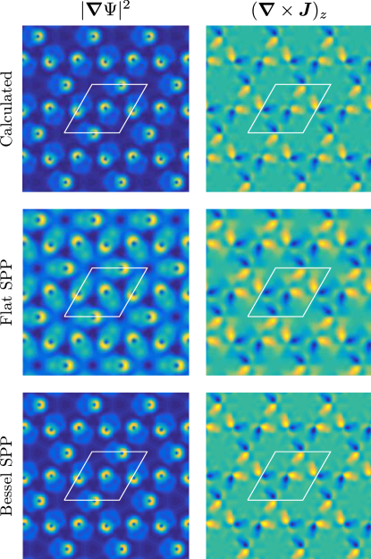
Figure 4: Comparison between $\left|\bm{\nabla}_{\perp}\Psi\right|^{2}$ and $(\bm{\nabla}\times\bm{J})_{z}$ calculated directly from the exit wave (top) and the average or difference of the SPP filtered images without (middle) and with Bessel modulated amplitude (bottom) ($k_{\text{max}}$=5 Å^-, $R=1\AA$).

In fig. 4 the average and the difference of the SPP filtered images with a flat or Bessel modulated amplitude are compared with the gradient of the exit wave squared, $\left|\bm{\nabla}_{\perp}\Psi\right|^{2}$, and the $z$-component of the curl of the probability current, $(\bm{\nabla}\times\bm{J})_{z}$, calculated directly from the exit wave. We can see that for both SPPs the average and difference are in good agreement with the calculated gradient and current vorticity images. For the flat SPPs a clear blurring of the images can be seen which is a direct consequence of the tails present in its Fourier transform, see fig. 1a. Since in our simulations $k_{\text{max}}$ is limited by the number of points and the resolution of the image, it can not be made arbitrarily large and these tails will remain to have a significant influence on the images. As argued before and shown in fig. 4, this blurring effect can be resolved by using a Bessel modulated amplitude SPP. Note that amplitude modulations is far more difficult and generally requires the use of a thin film of transparent material, introducing an increased sensitivity to beam damage and contamination in contrast to flat intensity SPPs, that can be created by magnetic needles or binary fork apertures.

V Image wave reconstruction

Whereas the amplitude of a wave can simply be measured by taking a conventional image, in which the intensity is given by

$$I=\left|\psi\right|^{2}=A^{2},$$ (19)

the phase is much harder to measure. However, as shown above, by inserting two oppositely handed SPPs, we get valuable extra information about the wave and the gradient of its amplitude and phase. Using $\frac{\partial{I}}{\partial{x}}=2A\frac{\partial{A}}{\partial{x}}$ we can rewrite eq. 17 and eq. 18 as

$$\begin{cases}\left[\frac{\partial{I}}{\partial{y}}\frac{\partial{\varphi}}{\partial{x}}-\frac{\partial{I}}{\partial{x}}\frac{\partial{\varphi}}{\partial{y}}\right]&=\frac{1}{2C}(I^{+}-I^{-})\\ \left(\frac{\partial{\varphi}}{\partial{x}}\right)^{2}+\left(\frac{\partial{\varphi}}{\partial{y}}\right)^{2}&=\frac{I^{+}+I^{-}}{2CI}-\left(\frac{1}{A}\frac{\partial{A}}{\partial{x}}\right)^{2}-\left(\frac{1}{A}\frac{\partial{A}}{\partial{y}}\right)^{2}\\ &=\frac{I^{+}+I^{-}}{2CI}-\frac{1}{4I^{2}}\left(\left(\frac{\partial{I}}{\partial{x}}\right)^{2}+\left(\frac{\partial{I}}{\partial{y}}\right)^{2}\right),\end{cases}$$ (20)

where $I$ is measured by taking a normal image without a SPP. Equation 20 represents a set of two first order partial differential equations that may be solved using the method of characteristics, thereby retrieving the phase $\varphi$. Note, however, that such a procedure is not straight forward. Problems may arise at crossing characteristics or at amplitude zeros, where the right hand side of the second equation diverges. A detailed elaboration on image wave reconstruction, lies beyond the scope of this paper.

VI Conclusion

In order to increase the contrast in optical and electron microscopy images, over the past decades several phase contrast techniques have been developed. In this work we study the effect of a spiral phase plate (SPP) that adds an angularly dependent phase to the wave in the Fourier plane of the form $e^{i\ell\phi}$. We analytically calculate the effect of an $\ell=\pm 1$ SPP in the limit for large $k_{\text{max}}$ and find that the average of two opposite SPP filtered images is equal to the square of the 2D gradient of the wave and that the difference is proportional to its current vorticity. The latter disappears when the 2D amplitude- and phase-gradient are parallel or if one of them is zero. We verified these analytical calculations on a simulated exit wave of a plane wave electron passing through a 20nm thick quartz crystal (fig. 4). Our calculations confirm the suggestion made by Fürhapter et al. Fürhapter et al. (2005) that for pure phase objects individual SPP filtered images are proportional to the gradient squared of the exit wave, but also show a further use for the spiral phase plate technique.

We demonstrated how an analysis of two opposite SPP filtered images enables detection of solenoidal currents, such as those occurring in combination with elastic scattering on magnetic samples or chiral inelastic excitations. Moreover, we indicate how the combination of a conventional image, an image with an $\ell=-1$ and an $\ell=1$ SPP might give enough information to reconstruct the entire exit wave, thereby opening new pathways to phase retrieval.

VII acknowledgments

The authors acknowledge support from the FWO (Aspirant Fonds Wetenschappelijk Onderzoek - Vlaanderen) and the EU under the Seventh Framework Program (FP7) under a contract for an Integrated Infrastructure Initiative, Reference No. 312483-ESTEEM2 and ERC Starting Grant 278510 VORTEX.

References

- Born and Wolf (1999) Max Born and Emil Wolf, Principles of Optics: Electromagnetic Theory of Propagation, Interference and Diffraction of Light, 7th ed. (Cambridge University Press, 1999).
- Martin (1966) L.C. Martin, Theory of the Microsope, 1st ed. (Blackie and Son, London, 1966) p. Chap. 7.
- Barer (1953) R. Barer, “A New Method of Light Microscopy,” Nature 171, 697–698 (1953).
- Danev and Nagayama (2001) Radostin Danev and Kuniaki Nagayama, “Transmission electron microscopy with Zernike phase plate,” Ultramicroscopy 88, 243–252 (2001).
- Danev and Nagayama (2008) Radostin Danev and Kuniaki Nagayama, “Single particle analysis based on Zernike phase contrast transmission electron microscopy,” Journal of Structural Biology 161, 211–218 (2008).
- Kaneko et al. (2006) Yasuko Kaneko, Radostin Danev, Kuniaki Nagayama, and Hitoshi Nakamoto, “Intact carboxysomes in a cyanobacterial cell visualized by Hilbert differential contrast transmission electron microscopy,” Journal of Bacteriology 188, 805–808 (2006).
- Zernike (1942a) F. Zernike, “Phase contrast, a new method for the microscopic observation of transparent objects part I,” Physica 9, 686–698 (1942a).
- Zernike (1942b) F. Zernike, “Phase contrast, a new method for the microscopic observation of transparent objects part II,” Physica 9, 974–986 (1942b).
- Pluta (1994) M. Pluta, “Nomarski’s DIC micmscopy: a review,” Proc. SPIE 1846, 10–25 (1994).
- Hoffman and Gross (1975) Robert Hoffman and Leo Gross, “Modulation Contrast Microscope,” Applied optics microscope 14, 1169–1176 (1975).
- Boersch (1947) Hans Boersch, “Über die Kontraste von Atomen im Elektronenmikroskop,” Zeitschrift fur Naturforschung - Section A Journal of Physical Sciences 2, 615–633 (1947).
- Matsumoto and Tonomura (1996) Takao Matsumoto and Akira Tonomura, “The phase constancy of electron waves traveling through Boersch’s electrostatic phase plate,” Ultramicroscopy 63, 5–10 (1996).
- Schultheiß et al. (2006) K. Schultheiß, F. Párez-Willard, B. Barton, D. Gerthsen, and R. R. Schröder, “Fabrication of a Boersch phase plate for phase contrast imaging in a transmission electron microscope,” Review of Scientific Instruments 77 (2006), 10.1063/1.2179411.
- Majorovits et al. (2007) E. Majorovits, B. Barton, K. Schultheiß, F. Pérez-Willard, D. Gerthsen, and R. R. Schröder, “Optimizing phase contrast in transmission electron microscopy with an electrostatic (Boersch) phase plate,” Ultramicroscopy 107, 213–226 (2007).
- Shimada et al. (2007) Atsushi Shimada, Hideaki Niwa, Kazuya Tsujita, Shiro Suetsugu, Koji Nitta, Kyoko Hanawa-Suetsugu, Ryogo Akasaka, Yuri Nishino, Mitsutoshi Toyama, Lirong Chen, Zhi Jie Liu, Bi Cheng Wang, Masaki Yamamoto, Takaho Terada, Atsuo Miyazawa, Akiko Tanaka, Sumio Sugano, Mikako Shirouzu, Kuniaki Nagayama, Tadaomi Takenawa, and Shigeyuki Yokoyama, “Curved EFC/F-BAR-Domain Dimers Are Joined End to End into a Filament for Membrane Invagination in Endocytosis,” Cell 129, 761–772 (2007).
- Yamaguchi et al. (2008) Masashi Yamaguchi, Radostin Danev, Kiyoto Nishiyama, Keishin Sugawara, and Kuniaki Nagayama, “Zernike phase contrast electron microscopy of ice-embedded influenza A virus,” Journal of Structural Biology 162, 271–276 (2008).
- Danev et al. (2014) Radostin Danev, Bart Buijsse, Maryam Khoshouei, Jürgen M Plitzko, and Wolfgang Baumeister, “Volta potential phase plate for in-focus phase contrast transmission electron microscopy.” Proceedings of the National Academy of Sciences of the United States of America 111, 15635–40 (2014).
- Asano et al. (2015) Shoh Asano, Yoshiyuki Fukuda, Florian Beck, Antje Aufderheide, Friedrich Förster, Radostin Danev, and Wolfgang Baumeister, “Proteasomes. A molecular census of 26S proteasomes in intact neurons.” Science (New York, N.Y.) 347, 439–42 (2015).
- Mahamid et al. (2016) J. Mahamid, S. Pfeffer, M. Schaffer, E. Villa, R. Danev, L. Kuhn Cuellar, F. Forster, A. A. Hyman, J. M. Plitzko, and W. Baumeister, “Visualizing the molecular sociology at the HeLa cell nuclear periphery,” Science 351, 969–972 (2016).
- Khoshouei et al. (2016) Maryam Khoshouei, Mazdak Radjainia, Amy J Phillips, Juliet A Gerrard, Alok K Mitra, Jürgen M Plitzko, Wolfgang Baumeister, and Radostin Danev, “Volta phase plate cryo-EM of the small protein complex Prx3.” Nature communications 7, 10534 (2016).
- Danev et al. (2002) R Danev, H Okawara, N Usuda, K Kametani, and K Nagayama, “A Novel Phase-contrast Transmission Electron Microscopy Producing High-contrast Topographic Images of Weak objects.” Journal of biological physics 28, 627–35 (2002).
- Kaneko et al. (2005) Yasuko Kaneko, Radostin Danev, Koji Nitta, and Kuniaki Nagayama, “In vivo subcellular ultrastructures recognized with Hilbert differential contrast transmission electron microscopy,” Journal of Electron Microscopy 54, 79–84 (2005).
- Nitta et al. (2009) K. Nitta, K. Nagayama, R. Danev, and Y. Kaneko, “Visualization of BrdU-labelled DNA in cyanobacterial cells by Hilbert differential contrast transmission electron microscopy,” Journal of Microscopy 234, 118–123 (2009).
- Davis et al. (2000) J a Davis, D E McNamara, D M Cottrell, and J Campos, “Image processing with the radial Hilbert transform: theory and experiments.” Optics letters 25, 99–101 (2000).
- Nye and Berry (1974) J. F. Nye and M. V. Berry, “Dislocations in Wave Trains,” Proceedings of the Royal Society A: Mathematical, Physical and Engineering Sciences 336, 165–190 (1974).
- Allen et al. (1992) L. Allen, M. W. Beijersbergen, R. J C Spreeuw, and J. P. Woerdman, “Orbital angular momentum of light and the transformation of Laguerre-Gaussian laser modes,” Physical Review A 45, 8185–8189 (1992).
- Galajda and Ormos (2001) Péter Galajda and Pál Ormos, “Complex micromachines produced and driven by light,” Applied Physics Letters 78, 249 (2001).
- Friese et al. (2001) M E J Friese, H Rubinsztein-Dunlop, J Gold, P Hagberg, and D Hanstorp, “Optically driven micromachine elements,” Applied Physics Letters 78, 547–549 (2001).
- Luo et al. (2000) Zong-Ping Luo, Yu-Long Sun, and Kai-Nan An, “An optical spin micromotor,” Appl. Phys. Lett. 76, 1779–1781 (2000).
- He et al. (1995) H He, M E J Friese, N R Heckenberg, and H Rubinsztein-Dunlop, “Direct Observation of Transfer of Angular Momentum to Absorptive Particles from a Laser Beam with a Phase Singularity,” Phys. Rev. Lett. 75, 826–829 (1995).
- Swartzlander and Hernandez-Aranda (2007) Grover Swartzlander and Raul Hernandez-Aranda, “Optical Rankine Vortex and Anomalous Circulation of Light,” Physical Review Letters 99, 163901 (2007).
- Serabyn et al. (2010) E Serabyn, D Mawet, and R Burruss, “An image of an exoplanet separated by two diffraction beamwidths from a star.” Nature 464, 1018–20 (2010).
- Berkhout and Beijersbergen (2008) Gregorius Berkhout and Marco Beijersbergen, “Method for Probing the Orbital Angular Momentum of Optical Vortices in Electromagnetic Waves from Astronomical Objects,” Phys. Rev. Lett. 101, 100801 (2008).
- Wang et al. (2012) Jian Wang, Jeng-Yuan Yang, Irfan M Fazal, Nisar Ahmed, Yan Yan, Hao Huang, Yongxiong Ren, Yang Yue, Samuel Dolinar, Moshe Tur, and Alan E Willner, “Terabit free-space data transmission employing orbital angular momentum multiplexing,” Nature Phot. 6, 488–496 (2012).
- Roychowdhury et al. (2004) Sanjoy Roychowdhury, Virendra K Jaiswal, and R.P. Singh, “Implementing controlled NOT gate with optical vortex,” Optics Communications 236, 419–424 (2004).
- Verbeeck et al. (2013) Jo Verbeeck, He Tian, and Gustaaf Van Tendeloo, “How to Manipulate Nanoparticles with an Electron Beam?” Advanced Materials 25, 1114–1117 (2013).
- Juchtmans et al. (2015) Roeland Juchtmans, Armand Béché, Artem Abakumov, Maria Batuk, and Jo Verbeeck, “Using electron vortex beams to determine chirality of crystals in transmission electron microscopy,” Phys. Rev. B 91, 94112 (2015).
- Fürhapter et al. (2005) Severin Fürhapter, Alexander Jesacher, Stefan Bernet, and Monika Ritsch-Marte, “Spiral phase contrast imaging in microscopy,” Optics Express 13, 689 (2005).
- Blackburn and Loudon (2014) A. M. Blackburn and J. C. Loudon, “Vortex beam production and contrast enhancement from a magnetic spiral phase plate,” Ultramicroscopy 136, 127–143 (2014).
- Juchtmans and Verbeeck (2015) Roeland Juchtmans and Jo Verbeeck, “Orbital angular momentum in electron diffraction and its use to determine chiral crystal symmetries,” Physical Review B 92, 134108 (2015).
- Nagayama (2008) Kuniaki Nagayama, “Development of phase plates for electron microscopes and their biological application,” European Biophysics Journal 37, 345–358 (2008).
- Béché et al. (2013) Armand Béché, Ruben Van Boxem, Gustaaf Van Tendeloo, and Jo Verbeeck, “Magnetic monopole field exposed by electrons,” Nature Physics 10, 26–29 (2013).
- Béché et al. (2016a) A. Béché, R. Juchtmans, and J. Verbeeck, “Efficient creation of electron vortex beams for high resolution STEM imaging,” Ultramicroscopy , 1–8 (2016a).
- Verbeeck et al. (2010) J Verbeeck, H Tian, and P Schattschneider, “Production and application of electron vortex beams.” Nature 467, 301–4 (2010).
- Béché et al. (2016b) A. Béché, R. Winkler, H. Plank, F. Hofer, and J. Verbeeck, “Focused electron beam induced deposition as a tool to create electron vortices,” Micron 80, 34–38 (2016b).
- Juchtmans and Verbeeck (2016) Roeland Juchtmans and Jo Verbeeck, “Local orbital angular momentum revealed by spiral phase plate imaging in transmission electron microscopy,” Phys. Rev. A 93, 023811 (2016), arXiv:1512.04789 .
- Wei et al. (2011) S B Wei, S W Zhu, and X-C Yuan, “Image edge enhancement in optical microscopy with a Bessel-like amplitude modulated spiral phase filter,” Journal of Optics 13, 105704 (2011).
- Grillo et al. (2014) Vincenzo Grillo, Ebrahim Karimi, Gian Carlo Gazzadi, Stefano Frabboni, Mark R. Dennis, and Robert W. Boyd, “Generation of nondiffracting electron bessel beams,” Physical Review X 4, 1–7 (2014).
- Lubk et al. (2015) A. Lubk, A. Béché, and J. Verbeeck, “Electron Microscopy of Probability Currents at Atomic Resolution,” Physical Review Letters 115, 1–5 (2015).
- Berry (2009) M V Berry, “Optical currents,” Journal of Optics A: Pure and Applied Optics 11, 094001 (2009).
- Misell (1976) D L Misell, “On the validity of the weak phase and other approximations in analysis of electron microscope images,” Journal of Physics D: Applied Physics 9, 1849–1866 (1976).
- Tonomura et al. (1986) Akira Tonomura, Tsuyoshi Matsuda, Junji Endo, Tatsuo Arii, and Kazuhiro Mihama, “Holographic interference electron microscopy for determining specimen magnetic structure and thickness distribution,” Physical Review B 34, 3397–3402 (1986).
- Dunin-Borkowski et al. (1998) R. E. Dunin-Borkowski, M. R. McCartney, B. Kardynal, and David J. Smith, “Magnetic interactions within patterned cobalt nanostructures using off-axis electron holography,” Journal of Applied Physics 84, 374 (1998).
- Rosenauer and Schowalter (2007) A Rosenauer and M Schowalter, “STEMSIM-a new software tool for simulation of STEM HAADF Z-contrast imaging,” in Springer Proceedings in Physics (Microscopy of Semiconducting Materials Conference, Cambridge) (2007).