Derivative-based Global Sensitivity Measures and Their Link with Sobol’ Sensitivity Indices

Abstract

The variance-based method of Sobol’ sensitivity indices is very popular among practitioners due to its efficiency and easiness of interpretation. However, for high-dimensional models the direct application of this method can be very time-consuming and prohibitively expensive to use. One of the alternative global sensitivity analysis methods known as the method of derivative based global sensitivity measures (DGSM) has recently become popular among practitioners. It has a link with the Morris screening method and Sobol’ sensitivity indices. DGSM are very easy to implement and evaluate numerically. The computational time required for numerical evaluation of DGSM is generally much lower than that for estimation of Sobol’ sensitivity indices. We present a survey of recent advances in DGSM and new results concerning new lower and upper bounds on the values of Sobol’ total sensitivity indices $S_{i}^{tot}$. Using these bounds it is possible in most cases to get a good practical estimation of the values of $S_{i}^{tot}$. Several examples are used to illustrate an application of DGSM.

Keywords: Global sensitivity analysis; Monte Carlo methods; Quasi Monte Carlo methods; Derivative based global measures; Morris method; Sobol’ sensitivity indices

1 Introduction

Global sensitivity analysis (GSA) is the study of how the uncertainty in the model output is apportioned to the uncertainty in model inputs Salt2008 ,Sobol2005 . GSA can provide valuable information regarding the dependence of the model output to its input parameters. The variance-based method of global sensitivity indices developed by Sobol’ Sobol1993 became very popular among practitioners due to its efficiency and easiness of interpretation. There are two types of Sobol’ sensitivity indices: the main effect indices, which estimate the individual contribution of each input parameter to the output variance, and the total sensitivity indices, which measure the total contribution of a single input factor or a group of inputs Homma1996 . The total sensitivity indices are used to identify non-important variables which can then be fixed at their nominal values to reduce model complexity Salt2008 . For high-dimensional models the direct application of variance-based GSA measures can be extremely time-consuming and impractical.

A number of alternative SA techniques have been proposed. In this paper we present derivative based global sensitivity measures (DGSM) and their link with Sobol’ sensitivity indices. DGSM are based on averaging local derivatives using Monte Carlo or Quasi Monte Carlo sampling methods. These measures were briefly introduced by Sobol’ and Gershman in Sobol1995 . Kucherenko et al Kuch2009 introduced some other derivative-based global sensitivity measures (DGSM) and coined the acronym DGSM. They showed that the computational cost of numerical evaluation of DGSM can be much lower than that for estimation of Sobol’ sensitivity indices which later was confirmed in other works Kiparis2009 . DGSM can be seen as a generalization and formalization of the Morris importance measure also known as elementary effects Morris1991 . Sobol’ and KucherenkoSobol2009 proved theoretically that there is a link between DGSM and the Sobol’ total sensitivity index $S_{i}^{tot}$ for the same input. They showed that DGSM can be used as an upper bound on total sensitivity index $S_{i}^{tot}$. They also introduced modified DGSM which can be used for both a single input and groups of inputs Sobol2010 . Such measures can be applied for problems with a high number of input variables to reduce the computational time. Lamboni et al Lamboni2013 extended results of Sobol’ and Kucherenko for models with input variables belonging to the class of Boltzmann probability measures.

The numerical efficiency of the DGSM method can be improved by using the automatic differentiation algorithm for calculation DGSM as was shown in Kiparis2009 . However, the number of required function evaluations still remains to be proportional to the number of inputs. This dependence can be greatly reduced using an approach based on algorithmic differentiation in the adjoint or reverse mode Griewank2008 . It allows estimating all derivatives at a cost at most 4-6 times of that for evaluating the original function Jansen2014 .

This paper is organised as follows: Section 2 presents Sobol’ global sensitivity indices. DGSM and lower and upper bounds on total Sobol’ sensitivity indices for uniformly distributed variables and random variables are presented in Sections 3 and 4, respectively. In Section 5 we consider test cases which illustrate an application of DGSM and their links with total Sobol’ sensitivity indices. Finally, conclusions are presented in Section 6.

2 Sobol’ global sensitivity indices

The method of global sensitivity indices developed by Sobol’ is based on ANOVA decomposition Sobol1993 . Consider the square integrable function $f({\rm{\bf x}})$ defined in the unit hypercube $H^{d}=[0,1]^{d}$. The decomposition of $f({\rm{\bf x}})$

$$f({\bf{x}})=f_{0}+\sum\limits_{i=1}^{d}{f_{i}(x_{i})}+\sum\limits_{i=1}^{d}{\sum\limits_{j>i}^{d}{f_{ij}(x_{i},x_{j})}}+\cdots+f_{12\cdots d}(x_{1},\cdots,x_{d}),$$ (1)

where $f_{0}=\int_{H^{d}}{f(x)dx}$ , is called ANOVA if conditions

$$\int_{H^{d}}{f_{i_{1}...i_{s}}dx_{i_{k}}}=0$$ (2)

are satisfied for all different groups of indices $x_{1},\cdots,x_{s}$ such that $1\leq i_{1}<i_{2}<...<i_{s}\leq d$. These conditions guarantee that all terms in (1) are mutually orthogonal with respect to integration.

The variances of the terms in the ANOVA decomposition add up to the total variance:

$$D=\int_{H^{d}}{f^{2}({\bf{x}})d}{\bf{x}}-f_{0}^{2}=\sum\limits_{s=1}^{d}{\sum\limits_{i_{1}<\cdot\cdot\cdot<i_{s}}^{d}{D_{i_{1}...i_{s}}}},$$

where $D_{i_{1}...i_{s}}=\int_{H^{d}}{f_{i_{1}...i_{s}}^{2}(x_{i_{1}},...,x_{i_{s}})dx_{i_{1}},...,x_{i_{s}}}$ are called partial variances.

Total partial variances account for the total influence of the factor $x_{i}$:

$$D_{i}^{tot}=\sum\limits_{<i>}{D_{i_{1}...i_{s}}},$$

where the sum $\sum\limits_{<i>}{}$ is extended over all different groups of indices $x_{1},\cdots,x_{s}$ satisfying condition $1\leq i_{1}<i_{2}<...<i_{s}\leq n$, $1\leq s\leq n$, where one of the indices is equal to $i$. The corresponding total sensitivity index is defined as

$$S_{i}^{tot}={{D_{i}^{tot}}\mathord{\left/{\vphantom{{D_{i}^{tot}}D}}\right.\kern-1.2pt}D}.$$

Denote $u_{i}({\bf{x}})$ the sum of all terms in ANOVA decomposition (1) that depend on $x_{i}$:

$$u_{i}({\bf{x}})=f_{i}(x_{i})+\sum\limits_{j=1,j\neq i}^{d}{f_{ij}(x_{i},x_{j})}+\cdots+f_{12\cdots d}(x_{1},\cdots,x_{d}).$$

From the definition of ANOVA decomposition it follows that

$$\int_{H^{d}}{u_{i}({\bf{x}})d{\bf{x}}}=0.$$ (3)

The total partial variance $D_{i}^{tot}$ can be computed as

$$D_{i}^{tot}=\int_{H^{d}}{u_{i}^{2}({\bf{x}})d{\bf{x}}}=\int_{H^{d}}{u_{i}^{2}(x_{i},{\bf{z}})dx_{i}d{\bf{z}}}.$$

Denote ${\bf{z}}=(x_{1},...,x_{i-1},x_{i+1},...,x_{d})$ the vector of all variables but $x_{i}$, then ${\bf{x}}\equiv(x_{i},{\bf{z}})$ and $f({\bf{x}})\equiv f(x_{i},{\bf{z}})$. The ANOVA decomposition of $f({\rm{\bf x}})$ in (1) can be presented in the following form

$$f({\bf{x}})=u_{i}(x_{i},{\bf{z}})+v({\bf{z}}),$$

where $v({\bf{z}})$ is the sum of terms independent of $x_{i}$. Because of (2) and (3) it is easy to show that $v({\bf{z}})=\int_{H^{d}}{f({\bf{x}})dx_{i}}$. Hence

$$u_{i}(x_{i},{\bf{z}})=f({\bf{x}})-\int_{H^{d}}{f({\bf{x}})dx_{i}}.$$ (4)

Then the total sensitivity index $S_{i}^{tot}$ is equal to

$$S_{i}^{tot}=\frac{{\int_{H^{d}}{u_{i}^{2}({\bf{x}})d{\bf{x}}}}}{D}.$$ (5)

We note that in the case of independent random variables all definitions of the ANOVA decomposition remain to be correct but all derivations should be considered in probabilistic sense as shown in Sobol2005 and presented in Section 4.

3 DGSM for uniformly distributed variables

Consider continuously differentiable function $f({\rm{\bf x}})$ defined in the unit hypercube $H^{d}=[0,1]^{d}$ such that ${{\partial f}\mathord{\left/{\vphantom{{\partial f}{\partial x_{i}}}}\right.\kern-1.2pt}{\partial x_{i}}}\in L_{2}$.

Theorem 3.1

Assume that $c\leq\left|{\frac{{\partial f}}{{\partial x_{i}}}}\right|\leq C$. Then

$$\frac{{c^{2}}}{{12D}}\leq S_{i}^{tot}\leq\frac{{C^{2}}}{{12D}}.$$ (6)

The proof is presented in Sobol2009 .

The Morris importance measure also known as elementary effects originally defined as finite differences averaged over a finite set of random points Morris1991 was generalized in Kuch2009 :

$$\mu_{i}=\int_{H^{d}}\left|{\frac{{\partial f({\bf{x}})}}{{\partial x_{i}}}}\right|d{\bf{x}}.$$ (7)

Kucherenko et al Kuch2009 also introduced a new DGSM measure:

$$\nu_{i}=\int_{H^{d}}{\left({\frac{{\partial f({\bf{x}})}}{{\partial x_{i}}}}\right)}^{2}d{\bf{x}}.$$ (8)

In this paper we define two new DGSM measures:

$$w_{i}^{(m)}=\int_{H^{d}}{x_{i}^{m}\frac{{\partial f({\bf{x}})}}{{\partial x_{i}}}d}{\bf{x}},$$ (9)

where $m$ is a constant, $m>0$,

$$\varsigma_{i}=\frac{1}{2}\int_{H^{d}}{x_{i}(1-x_{i})\left({\frac{{\partial f({\bf{x}})}}{{\partial x_{i}}}}\right)^{2}d}{\bf{x}}.$$ (10)

We note that $\nu_{i}$ is in fact the mean value of $\left({{{\partial f}\mathord{\left/{\vphantom{{\partial f}{\partial x_{i}}}}\right.\kern-1.2pt}{\partial x_{i}}}}\right)^{2}$. We also note that

$$\frac{{\partial f}}{{\partial x_{i}}}=\frac{{\partial u_{i}}}{{\partial x_{i}}}.$$ (11)

3.1 Lower bounds on $S_{i}^{tot}$

Theorem 3.2

There exists the following lower bound between DGSM (8) and the Sobol’ total sensitivity index

$$\frac{{\left({\int_{H^{d}}{\left[{f\left({1,{\bf{z}}}\right)-f\left({0,{\bf{z}}}\right)}\right]\left[{f\left({1,{\bf{z}}}\right)+f\left({0,{\bf{z}}}\right)-2f\left({\bf{x}}\right)}\right]d}{\bf{x}}}\right)^{2}}}{{4\nu_{i}D}}<S_{i}^{tot}.$$ (12)

Proof

Consider an integral

$$\int_{H^{d}}{u_{i}({\bf{x}})\frac{{\partial u_{i}({\bf{x}})}}{{\partial x_{i}}}}d{\bf{x}}.$$ (13)

Applying the Cauchy–Schwarz inequality we obtain the following result:

$$\left({\int_{H^{d}}{u_{i}({\bf{x}})\frac{{\partial u_{i}({\bf{x}})}}{{\partial x_{i}}}}d{\bf{x}}}\right)^{2}\leq\int_{H^{d}}{u_{i}^{2}({\bf{x}})}d{\bf{x}}\cdot\int_{H^{d}}{\left({\frac{{\partial u_{i}({\bf{x}})}}{{\partial x_{i}}}}\right)}^{2}d{\bf{x}}.$$ (14)

It is easy to prove that the left and right parts of this inequality cannot be equal. Indeed, for them to be equal functions $u_{i}({\bf{x}})$ and $\frac{{\partial u_{i}({\bf{x}})}}{{\partial x_{i}}}$ should be linearly dependent. For simplicity consider a one-dimensional case: $x\in[0,1]$. Let’s assume

$$\frac{{\partial u(x)}}{{\partial x}}=Au(x),$$

where $A$ is a constant. The general solution to this equation $u(x)=B\exp(Ax)$ , where $B$ is a constant. It is easy to see that this solution is not consistent with condition (3) which should be imposed on function $u(x)$.

Integral $\int_{H^{d}}{u_{i}({\bf{x}})\frac{{\partial u_{i}({\bf{x}})}}{{\partial x_{i}}}}d{\bf{x}}$ can be transformed as

$$\begin{array}[]{l}\int_{H^{d}}{u_{i}({\bf{x}})\frac{{\partial u_{i}({\bf{x}})}}{{\partial x_{i}}}}d{\bf{x}}=\frac{1}{2}\int_{H^{d}}{\frac{{\partial u_{i}^{2}({\bf{x}})}}{{\partial x_{i}}}}d{\bf{x}}\\ =\frac{1}{2}\int_{H^{d-1}}{\left({u_{i}^{2}(1,{\bf{z}})-u_{i}^{2}(0,{\bf{z}})}\right)d{\bf{z}}}\\ =\frac{1}{2}\int_{H^{d-1}}{\left({u_{i}(1,{\bf{z}})-u_{i}(0,{\bf{z}})}\right)\left({u_{i}(1,{\bf{z}})+u_{i}(0,{\bf{z}})}\right)d{\bf{z}}}\\ =\frac{1}{2}\int_{H^{d}}{\left({f(1,{\bf{z}})-f(0,{\bf{z}})}\right)\left({f(1,{\bf{z}})+f(0,{\bf{z}})-2v({\bf{z}})}\right)d{\bf{z}}.}\\ \end{array}$$ (15)

All terms in the last integrand are independent of $x_{i}$, hence we can replace integration with respect to $d{\bf{z}}$ to integration with respect to $d{\bf{x}}$ and substitute $v({\bf{z}})$ for $f({\bf{x}})$ in the integrand due to condition (3). Then (15) can be presented as

$$\int_{H^{d}}{u_{i}({\bf{x}})\frac{{\partial u_{i}({\bf{x}})}}{{\partial x_{i}}}}d{\bf{x}}=\frac{1}{2}\int_{H^{d}}{\left[{f\left({1,{\bf{z}}}\right)-f\left({0,{\bf{z}}}\right)}\right]\left[{f\left({1,{\bf{z}}}\right)+f\left({0,{\bf{z}}}\right)-2f\left({\bf{x}}\right)}\right]d}{\bf{x}}$$ (16)

From (11) $\frac{{\partial u_{i}({\bf{x}})}}{{\partial x_{i}}}=\frac{{\partial f({\bf{x}})}}{{\partial x_{i}}}$, hence the right hand side of (14) can be written as $\nu_{i}D_{i}^{tot}$. Finally dividing (14) by $\nu_{i}D$ and using (16), we obtain the lower bound (12). ∎

We call

$$\frac{{\left({\int_{H^{d}}{\left[{f\left({1,{\bf{z}}}\right)-f\left({0,{\bf{z}}}\right)}\right]\left[{f\left({1,{\bf{z}}}\right)+f\left({0,{\bf{z}}}\right)-2f\left({\bf{x}}\right)}\right]d}{\bf{x}}}\right)^{2}}}{{4\nu_{i}D}}$$

the lower bound number one (LB1).

Theorem 3.3

There exists the following lower bound between DGSM (9) and the Sobol’ total sensitivity index

$$\frac{{(2m+1)\left[{\int_{H^{d}}{\left({f(1,{\bf{z}})-f({\bf{x}})}\right)d{\bf{x}}}-w_{i}^{(m+1)}}\right]^{2}}}{{(m+1)^{2}D}}<S_{i}^{tot}$$ (17)

Proof

Consider an integral

$$\int_{H^{d}}{x_{i}^{m}u_{i}({\bf{x}})d}{\bf{x}}.$$ (18)

Applying the Cauchy–Schwarz inequality we obtain the following result:

$$\left({\int_{H^{d}}{x_{i}^{m}u_{i}({\bf{x}})d}{\bf{x}}}\right)^{2}\leq\int_{H^{d}}{x_{i}^{2m}d}{\bf{x}}\cdot\int_{H^{d}}{u_{i}^{2}({\bf{x}})d}{\bf{x}}.$$ (19)

It is easy to see that equality in (19) cannot be attained. For this to happen functions $u_{i}({\bf{x}})$ and $x_{i}^{m}$ should be linearly dependent. For simplicity consider a one-dimensional case: $x\in[0,1]$. Let’s assume

$$u(x)=Ax^{m},$$

where $A\neq 0$ is a constant. This solution does not satisfy condition (3) which should be imposed on function $u(x)$.

Further we use the following transformation:

$$\int_{H^{d}}{\frac{{\partial\left({x_{i}^{m+1}u_{i}({\bf{x}})}\right)}}{{\partial x_{i}}}d}{\bf{x}}=(m+1)\int_{H^{d}}{x_{i}^{m}u_{i}({\bf{x}})d}{\bf{x}}+\int_{H^{d}}{x_{i}^{m+1}\frac{{\partial u_{i}({\bf{x}})}}{{\partial x_{i}}}d}{\bf{x}}$$

to present integral (18) in a form:

$$\begin{array}[]{l}\int_{H^{d}}{x_{i}^{m}u_{i}({\bf{x}})d}{\bf{x}}=\frac{1}{{m+1}}\left[{\int_{H^{d}}{\frac{{\partial\left({x_{i}^{m+1}u_{i}({\bf{x}})}\right)}}{{\partial x_{i}}}d}{\bf{x}}-\int_{H^{d}}{x_{i}^{m+1}\frac{{\partial u_{i}({\bf{x}})}}{{\partial x_{i}}}d}{\bf{x}}}\right]\\ =\frac{1}{{m+1}}\left[{\int_{H^{d-1}}{u_{i}(1,{\bf{z}})d}{\bf{z}}-\int_{H^{d}}{x_{i}^{m+1}\frac{{\partial u_{i}({\bf{x}})}}{{\partial x_{i}}}d}{\bf{x}}}\right]\\ =\frac{1}{{m+1}}\left[{\int_{H^{d}}{\left({f(1,{\bf{z}})-f({\bf{x}})}\right)d{\bf{x}}}-\int_{H^{d}}{x_{i}^{m+1}\frac{{\partial u_{i}({\bf{x}})}}{{\partial x_{i}}}d}{\bf{x}}}\right].\\ \end{array}$$ (20)

We notice that

$$\int_{H^{d}}{x_{i}^{2m}d}{\bf{x}}=\frac{1}{{(2m+1)}}.$$ (21)

Using (20) and (21) and dividing (19) by $D$ we obtain (17). ∎

This second lower bound on $S_{i}^{tot}$ we denote $\gamma(m)$:

$$\gamma(m)=\frac{{(2m+1)\left[{\int_{H^{d}}{\left({f(1,{\bf{z}})-f({\bf{x}})}\right)d{\bf{x}}}-w_{i}^{(m+1)}}\right]^{2}}}{{(m+1)^{2}D}}<S_{i}^{tot}.$$ (22)

In fact, this is a set of lower bounds depending on parameter $m$. We are interested in the value of $m$ at which $\gamma(m)$ attains its maximum. Further we use star to denote such a value $m$: $m^{*}=\arg\max(\gamma(m))$ and call

$$\gamma^{*}(m^{*})=\frac{{(2m^{*}+1)\left[{\int_{H^{d}}{\left({f(1,{\bf{z}})-f({\bf{x}})}\right)d{\bf{x}}}-w_{i}^{(m^{*}+1)}}\right]^{2}}}{{(m^{*}+1)^{2}D}}$$ (23)

the lower bound number two (LB2).

We define the maximum lower bound $LB^{*}$ as

$$LB^{*}=max(LB1,LB2).$$ (24)

We note that both lower and upper bounds can be estimated by a set of derivative based measures:

$$\Upsilon_{i}=\{\nu_{i},w_{i}^{(m)}\},{\rm{}}m>0.$$ (25)

3.2 Upper bounds on $S_{i}^{tot}$

Theorem 3.4

$$S_{i}^{tot}\leq\frac{{\nu_{i}}}{{\pi^{2}D}}.$$ (26)

The proof of this Theorem in given in Sobol2009 .

Consider the set of values $\nu_{1},...,\nu_{n}$, $1\leq i\leq n$. One can expect that smaller $\nu_{i}$ correspond to less influential variables $x_{i}$.

We further call (26) the upper bound number one (UB1).

Theorem 3.5

$$S_{i}^{tot}\leq\frac{{\varsigma_{i}}}{D},$$ (27)

where $\varsigma_{i}$ is given by (10).

Proof

We use the following inequality Hardy1973 :

$$0\leq\int_{0}^{1}{u^{2}dx}-\left({\int_{0}^{1}{udx}}\right)^{2}\leq\frac{1}{2}\int_{0}^{1}{x(1-x)u^{\prime 2}dx}.$$ (28)

The inequality is reduced to an equality only if $u$ is constant. Assume that $u$ is given by (3), then $\int_{0}^{1}{udx}=0$, and from (28) we obtain (27). ∎

Further we call $\frac{{\varsigma_{i}}}{D}$ the upper bound number two (UB2). We note that $\frac{1}{2}x_{i}(1-x_{i})$ for $0\leq x_{i}\leq 1$ is bounded: $0\leq\frac{1}{2}x_{i}(1-x_{i})\leq\frac{1}{8}$. Therefore, $0\leq\varsigma_{i}\leq\frac{1}{8}\nu_{i}$.

3.3 Computational costs

All DGSM can be computed using the same set of partial derivatives $\frac{{\partial f(x)}}{{\partial x_{i}}},{\rm{}}i=1,...,d$. Evaluation of $\frac{{\partial f(x)}}{{\partial x_{i}}}$ can be done analytically for explicitly given easily-differentiable functions or numerically.

In the case of straightforward numerical estimations of all partial derivatives and computation of integrals using MC or QMC methods, the number of required function evaluations for a set of all input variables is equal to $N(d+1)$, where $N$ is a number of sampled points. Computing LB1 also requires values of $f\left({0,z}\right),f\left({1,z}\right)$, while computing LB2 requires only values of $f\left({1,z}\right)$. In total, numerical computation of $LB^{*}$ for all input variables would require $N_{F}^{LB^{*}}=N(d+1)+2Nd=N(3d+1)$ function evaluations. Computation of all upper bounds require $N_{F}^{UB}=N(d+1)$ function evaluations. We recall that the number of function evaluations required for computation of $S_{i}^{tot}$ is $N_{F}^{S}=N(d+1)$ Salt2010 . The number of sampled points $N$ needed to achieve numerical convergence can be different for DGSM and $S_{i}^{tot}$. It is generally lower for the case of DGSM. The numerical efficiency of the DGSM method can be significantly increased by using algorithmic differentiation in the adjoint (reverse) mode Griewank2008 . This approach allows estimating all derivatives at a cost at most 6 times of that for evaluating the original function $f(x)$ Jansen2014 . However, as mentioned above lower bounds also require computation of $f\left({0,z}\right),f\left({1,z}\right)$ so $N_{F}^{LB^{*}}$ would only be reduced to $N_{F}^{LB^{*}}=6N+2Nd=N(2d+6)$, while $N_{F}^{UB}$ would be equal to $6N$.

4 DGSM for random variables

Consider a function $f\left({x_{1},...,x_{d}}\right)$, where $x_{1},...,x_{d}$ are independent random variables with distribution functions $F_{1}\left({x_{1}}\right),...,F_{d}\left({x_{d}}\right)$. Thus the point ${\bf{x}}=(x_{1},...,x_{d})$ is defined in the Euclidean space $R^{d}$ and its measure is $dF_{1}\left({x_{1}}\right)\cdot\cdot\cdot dF_{d}\left({x_{d}}\right)$.

The following DGSM was introduced in Sobol2009 :

$$\nu_{i}=\int_{R^{d}}{\left({\frac{{\partial f({\bf{x}})}}{{\partial x_{i}}}}\right)^{2}d}F({\bf{x}}).$$ (29)

We introduce a new measure

$$w_{i}=\int_{R^{d}}{\frac{{\partial f({\bf{x}})}}{{\partial x_{i}}}d}F({\bf{x}}).$$ (30)

4.1 The lower bounds on $S_{i}^{tot}$ for normal variables

Assume that $x_{i}$ is normally distributed with the finite variance $\sigma_{i}^{2}$ and the mean value $\mu_{i}$.

Theorem 4.1

$$\frac{{\sigma_{i}^{2}w_{i}^{2}}}{D}\leq S_{i}^{tot}.$$ (31)

Proof

Consider $\int_{R^{d}}{x_{i}u_{i}({\bf{x}})d}F({\bf{x}})$. Applying the Cauchy–Schwarz inequality we obtain

$$\left({\int_{R^{d}}{x_{i}u_{i}({\bf{x}})d}F({\bf{x}})}\right)^{2}\leq\int_{R^{d}}{x_{i}^{2}d}F({\bf{x}})\cdot\int_{R^{d}}{u_{i}^{2}({\bf{x}})d}F({\bf{x}}).$$ (32)

Equality in (32) can be attained if functions $u_{i}({\bf{x}})$ and $x_{i}$ are linearly dependent. For simplicity consider a one-dimensional case. Let’s assume

$$u(x)=A(x-\mu),$$

where $A\neq 0$ is a constant. This solution satisfies condition (3) for normally distributed variable $x$ with the mean value $\mu$: $\int_{R^{d}}{u(x)dF(x)}=0$.

For normally distributed variables the following equality is true Hardy1973 :

$$\left({\int_{R^{d}}{x_{i}u_{i}({\bf{x}})d}F({\bf{x}})}\right)^{2}=\int_{R^{d}}{x_{i}^{2}d}F({\bf{x}})\cdot\int_{R^{d}}{\frac{{\partial u_{i}({\bf{x}})}}{{\partial x_{i}}}d}F({\bf{x}}).$$ (33)

By definition $\int_{R^{d}}{x_{i}^{2}d}F({\bf{x}})=\sigma_{i}^{2}$. Using (32) and (33) and dividing the resulting inequality by $D$ we obtain the lower bound (31). ∎

4.2 The upper bounds on $S_{i}^{tot}$ for normal variables

The following Theorem 7 is a generalization of Theorem 1.

Theorem 4.2

Assume that $c\leq\left|{\frac{{\partial f}}{{\partial x_{i}}}}\right|\leq C$, then

$$\frac{{\sigma_{i}^{2}c^{2}}}{D}\leq S_{i}^{tot}\leq\frac{{\sigma_{i}^{2}C^{2}}}{D}.$$ (34)

The constant factor $\sigma_{i}^{2}$ cannot be improved.

Theorem 4.3

$$S_{i}^{tot}\leq\frac{{\sigma_{i}^{2}}}{D}\nu_{i}.$$ (35)

The constant factor $\sigma_{i}^{2}$ cannot be reduced.

Proofs are presented in Sobol2009 .

5 Test cases

In this section we present the results of analytical and numerical estimation of $S_{i}$, $S_{i}^{tot}$, LB1, LB2 and UB1, UB2. The analytical values for DGSM and $S_{i}^{tot}$ were calculated and compared with numerical results. For text case 2 we present convergence plots in the form of root mean square error (RMSE) versus the number of sampled points $N$. To reduce the scatter in the error estimation the values of RMSE were averaged over $K$ = 25 independent runs:

$$\varepsilon_{i}=\left({\frac{1}{K}\sum\limits_{k=1}^{K}{\left({\frac{{I_{i,k}^{*}-I_{0}}}{{I_{0}}}}\right)^{2}}}\right)^{\frac{1}{2}}.$$

Here $I_{i}^{*}$ is numerically computed values of $S_{i}^{tot}$, LB1, LB2 or UB1, UB2, $I_{0}$ is the corresponding analytical value of $S_{i}^{tot}$, LB1, LB2 or UB1, UB2. The RMSE can be approximated by a trend line $cN^{-\alpha}$. Values of ($-\alpha)$ are given in brackets on the plots. QMC integration based on Sobol’ sequences was used in all numerical tests.

Example 1. Consider a linear with respect to $x_{i}$ function:

$$f({\bf{x}})=a(z)x_{i}+b(z).$$

For this function $S_{i}=S_{i}^{tot}$, $D_{i}^{tot}=\frac{1}{{12}}\int_{H^{d-1}}{a^{2}(z)dz}$, $\nu_{i}=\int_{H^{d-1}}{a^{2}(z)dz}$, $LB1=\frac{{\left({\int_{H^{d}}{\left({a^{2}(z)-2a^{2}(z)x_{i}}\right)dzdx_{i}}}\right)^{2}}}{{4D\int_{H^{d-1}}{a^{2}(z)dz}}}=0$ and $\gamma(m)=\frac{{(2m+1)m^{2}\left({\int_{H^{d-1}}{a(z)dz}}\right)^{2}}}{{4(m+2)^{2}(m+1)^{2}D}}$. A maximum value of $\gamma(m)$ is attained at $m^{*}$=3.745, when $\gamma^{*}(m^{*})=\frac{{0.0401}}{D}\left({\int{a(z)dz}}\right)^{2}$. The lower and upper bounds are $LB*\approx{\rm{0}}{\rm{.48}}S_{i}^{tot}$. $UB1\approx 1.{\rm{22}}S_{i}^{tot}$. $UB2=\frac{1}{{12D}}\int_{0}^{1}{a(z)^{2}dz}=S_{i}^{tot}$. For this test function UB2 $<$ UB1.

Example 2. Consider the so-called g-function which is often used in GSA for illustration purposes:

$$f({\bf{x}})=\prod\limits_{i=1}^{d}{g_{i}},$$

where $g_{i}=\frac{{|4x_{i}-2|+a_{i}}}{{1+a_{i}}}$, $a_{i}(i=1,...,d)$ are constants. It is easy to see that for this function $f_{i}(x_{i})=(g_{i}-1)$, $u_{i}({\bf{x}})=(g_{i}-1)\prod\limits_{j=1,j\neq i}^{d}{g_{j}}$ and as a result LB1=0. The total variance is $D=-1+\prod\limits_{j=1}^{d}{\left({1+\frac{{1/3}}{{(1+a_{j})^{2}}}}\right)}$. The analytical values of $S_{i}$, $S_{i}^{tot}$ and LB2 are given in Table 1.

Table 1: The analytical expressions for $S_{i}$, $S_{i}^{tot}$ and LB2 for g-function

$S_{i}$	$S_{i}^{tot}$	$\gamma(m)$
$\displaystyle\frac{{1/3}}{{(1+a_{i})^{2}D}}$	$\displaystyle\frac{{\frac{{1/3}}{{(1+a_{i})^{2}}}\prod\limits_{j=1,j\neq i}^{d}{\left({1+\frac{{1/3}}{{(1+a_{j})^{2}}}}\right)}}}{D}$	$\displaystyle\frac{{(2m+1)\left[{1-\frac{{4\left({1-(1/2)^{m+1}}\right)}}{{m+2}}}\right]^{2}}}{{(1+a_{i})^{2}(m+1)^{2}D}}$

By solving equation $\frac{{d\gamma(m)}}{{dm}}=0$ , we find that $m^{*}$=9.64, $\gamma(m^{*})=\frac{{0.0772}}{{(1+a_{i})^{2}D}}$. It is interesting to note that $m^{*}$ does not depend on $a_{i}$, $i=1,2,...,d$ and $d$. In the extreme cases: if $a_{i}\to\infty$ for all $i$, $\frac{{\gamma(m^{*})}}{{S_{i}^{tot}}}\to 0.257$, $\frac{{S_{i}}}{{S_{i}^{tot}}}\to 1$, while if $a_{i}\to 0$ for all $i$, $\frac{{\gamma(m^{*})}}{{S_{i}^{tot}}}\to\frac{{0.257}}{{(4/3)^{d-1}}}$, $\frac{{S_{i}}}{{S_{i}^{tot}}}\to\frac{1}{{(4/3)^{d-1}}}$. The analytical expression for $S_{i}^{tot}$, UB1 and UB2 are given in Table 2.

Table 2: The analytical expressions for $S_{i}^{tot}$ UB1 and UB2 for g-function

$S_{i}^{tot}$	$UB1$	$UB2$
$\displaystyle\frac{{\frac{{1/3}}{{(1+a_{i})^{2}}}\prod\limits_{j=1,j\neq i}^{d}{\left({1+\frac{{1/3}}{{(1+a_{j})^{2}}}}\right)}}}{D}$	$\displaystyle\frac{{16\prod\limits_{j=1,j\neq i}^{d}{\left({1+\frac{{1/3}}{{(1+a_{j})^{2}}}}\right)}}}{{(1+a_{i})^{2}\pi^{2}D}}$	$\displaystyle\frac{{4\prod\limits_{j=1,j\neq i}^{d}{\left({1+\frac{{1/3}}{{(1+a_{j})^{2}}}}\right)}}}{{3(1+a_{i})^{2}D}}$

For this test function $\frac{{S_{i}^{tot}}}{{{\rm{UB1}}}}=\frac{{\pi^{2}}}{{48}}$, $\frac{{S_{i}^{tot}}}{{{\rm{UB2}}}}=\frac{1}{4}$, hence $\frac{{{\rm{UB2}}}}{{{\rm{UB1}}}}=\frac{{\pi^{2}}}{{12}}<1$. Values of $S_{i}$, $S_{i}^{tot}$, UB and LB2 for the case of a=[0,1,4.5,9,99,99,99,99], $d$=8 are given in Table 3 and shown in Figure 1. We can conclude that for this test function the knowledge of LB2 and UB1, UB2 allows to rank correctly all the variables in the order of their importance.

Table 3: Values of LB*, $S_{i}$, $S_{i}^{tot}$ , UB1 and UB1. Example 2, a=[0,1,4.5,9,99,99,99,99], $d$=8.

	$x_{1}$	$x_{2}$	$x_{3}$	$x_{4}$	$x_{5}...x_{8}$
$LB^{*}$	$0.166$	$0.0416$	$0.00549$	$0.00166$	$0.000017$
$S_{i}$	$0.716$	$0.179$	$0.0237$	$0.00720$	$0.0000716$
$S_{i}^{tot}$	$0.788$	$0.242$	$0.0343$	$0.0105$	$0.000105$
$UB1$	$3.828$	$1.178$	$0.167$	$0.0509$	$0.000501$
$UB2$	$3.149$	$0.969$	$0.137$	$0.0418$	$0.00042$

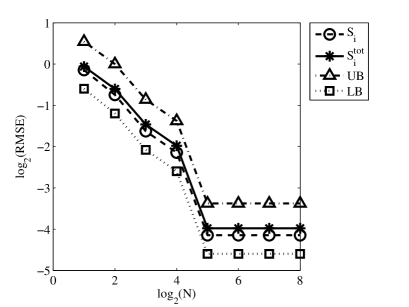
Figure 1: Values of $S_{i}$,$S_{i}^{tot}$, LB2 and UB1 for all input variables. Example 2, a=[0,1,4.5,9,99,99,99,99], $d$=8.

Fig. 2 presents RMSE of numerical estimations of $S_{i}^{tot}$, UB1 and LB2. For an individual input LB2 has the highest convergence rate, following by $S_{i}^{tot}$, and UB1 in terms of the number of sampled points. However, we recall that computation of all indices requires $N_{F}^{LB*}=N(3d+1)$ function evaluations for LB, while for $S_{i}^{tot}$ this number is $N_{F}^{S}=N(d+1)$ and for UB it is also $N_{F}^{UB}=N(d+1)$.

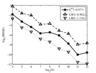
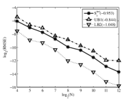
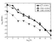
Figure 2: RMSE of $S_{i}^{tot}$, UB and LB2 versus the number of sampled points. Example 2, a=[0,1,4.5,9,99,99,99,99], $d$=8. Variable 1 (a), variable 3 (b) and variable 5 (c).

Example 3. Hartmann function $f({\bf{x}})=-\sum\limits_{i=1}^{4}{c_{i}\exp\left[{-\sum\limits_{j=1}^{n}{\alpha_{ij}(x_{j}-p_{ij})^{2}}}\right]}$, $x_{i}\in[0,1]$. For this test case a relationship between the values LB1, LB2 and $S_{i}$ varies with the change of input (Table 4, Figure 3): for variables $x_{2}$ and $x_{6}$ LB1$>$ $S_{i}$$>$ LB2, while for all other variables LB1$<$ LB2 $<$$S_{i}$. LB* is much smaller than $S_{i}^{tot}$ for all inputs. Values of $m$* also vary with the change of input. For all variables but variable 2 UB1 $>$ UB2.

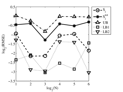
Figure 3: Values of $S_{i}$,$S_{i}^{tot}$, UB1, LB1 and LB2 for all input variables. Example 3.

Table 4: Values of $m^{*}$, LB1, LB2, UB1, UB2,$S_{i}$ and $S_{i}^{tot}$ for all input variables.

	$x_{1}$	$x_{2}$	$x_{3}$	$x_{4}$	$x_{5}$	$x_{6}$
$LB1$	$0.0044$	$0.0080$	$0.0009$	$0.0029$	$0.0014$	$0.0357$
$LB2$	$0.0515$	$0.0013$	$0.0011$	$0.0418$	$0.0390$	$0.0009$
$m^{*}$	$4.6$	$10.2$	$17.0$	$5.5$	$3.6$	$19.9$
$LB^{*}$	$0.0515$	$0.0080$	$0.0011$	$0.0418$	$0.0390$	$0.0357$
$S_{i}$	$0.115$	$0.00699$	$0.00715$	$0.0888$	$0.109$	$0.0139$
$S_{i}^{tot}$	$0.344$	$0.398$	$0.0515$	$0.381$	$0.297$	$0.482$
$UB1$	$1.089$	$0.540$	$0.196$	$1.088$	$1.073$	$1.046$
$UB2$	$1.051$	$0.550$	$0.150$	$0.959$	$0.932$	$0.899$

6 Conclusions

We can conclude that using lower and upper bounds based on DGSM it is possible in most cases to get a good practical estimation of the values of $S_{i}^{tot}$ at a fraction of the CPU cost for estimating $S_{i}^{tot}$. Small values of upper bounds imply small values of $S_{i}^{tot}$. DGSM can be used for fixing unimportant variables and subsequent model reduction. For linear function and product function, DGSM can give the same variable ranking as $S_{i}^{tot}$. In a general case variable ranking can be different for DGSM and variance based methods. Upper and lower bounds can be estimated using MC/QMC integration methods using the same set of partial derivative values. Partial derivatives can be efficiently estimated using algorithmic differentiation in the reverse (adjoint) mode.

We note that all bounds should be computed with sufficient accuracy. Standard techniques for monitoring convergence and accuracy of MC/QMC estimates should be applied to avoid erroneous results.

References

(1)
A. Griewank and A. Walther.
Evaluating derivatives: Principles and techniques
of algorithmic differentiation.SIAM Philadelphia, PA, 2008.
(2)
G.H. Hardy, J.E. Littlewood and G. Polya.
Inequalities.Cambridge University Press, Second edition, 1973.
(3)
T. Homma and A. Saltelli.
Importance measures in global sensitivity analysis of
model output.
Reliability Engineering and System Safety, 52(1):1–17, 1996.
(4)
K. Jansen, H. Leovey, A. Nube, A. Griewank. and M. Mueller-Preussker.
A first look at quasi-Monte Carlo for lattice field theory problems.
Comput. Phys. Commun., 185:948–959, 2014.
(5)
A. Kiparissides, S. Kucherenko, A. Mantalaris and E.N. Pistikopoulos.