Action Classification via Concepts and Attributes

Abstract

Classes in natural images tend to follow long tail distributions. This is problematic when there are insufficient training examples for rare classes. This effect is emphasized in compound classes, involving the conjunction of several concepts, such as those appearing in action-recognition datasets. In this paper, we propose to address this issue by learning how to utilize common visual concepts which are readily available. We detect the presence of prominent concepts in images and use them to infer the target labels instead of using visual features directly, combining tools from vision and natural-language processing. We validate our method on the recently introduced HICO dataset reaching a mAP of 31.54% and on the Stanford-40 Actions dataset, where the proposed method outperforms that obtained by direct visual features, obtaining an accuracy 83.12%. Moreover, the method provides for each class a semantically meaningful list of keywords and relevant image regions relating it to its constituent concepts.

I Introduction

In many tasks in pattern recognition, and specifically in computer vision, target classes follow a long-tail distribution. In the domain of action recognition this particularly true since the product of actions and objects is much bigger than each alone, and some examples may not be observed at all. This has been observed in several studies [21, 28, 24] and it is becoming increasingly popular to overcome this problem by building ever larger datasets [15, 22]. However, the distribution of these datasets will inevitably be long-tailed as well. One way to tackle this problem is to borrow information from external data sources. For instance, it has become popular to combine language and vision using joint embedded spaces [18, 14], which allow recognizing unseen classes more reliably than using a purely visual approach.

In this work, we propose to use an annotated concept dataset to learn a mapping from images to concepts with a visual meaning (e.g., objects and object attributes). This mapping is then used as a feature representation for classifying a target dataset, instead of describing the images with visual features extracted directly. This allows to describe an image or scene directly with high-level concepts instead of using visual features directly for the task. We show that training image classifiers this way, specifically in action-recognition, is as effective as training on the visual features. Moreover, we show that the concepts learned to be relevant to each category carry semantic meaning, which enables us to gain further insights into their success and failure modes. Our concept dataset is the Visual-Genome dataset [11], in which we leverage the rich region annotations.

II Previous Work

We list several lines of word related to ours. An early related work is ObjectBank [13], where the outputs of detectors for 200 common objects are aggregated via a spatial-pyramid to serve as feature representations. In the same spirit, ActionBank [23] learns detectors for various action types in videos and uses them to represent others as weighted combinations of actions. The work of [12] learns object attributes to describe objects in a zero-shot learning setting, so that new classes (animals) can be correctly classified by matching them to human generated lists of attributes. Recently, [21] learned various types of relations between actions (e.g., part of / type of / mutually exclusive) via visual and linguistic cues and leveraged those to be able to retrieve images of actions from a very large variety (27k) of action descriptions. Recent works have shown that emergent representations in deep networks tend to align with semantic concepts, such as textures, object parts and entire objects [2], confirming that it may prove useful to further guide a classifier of a certain class with semantically related concepts. Other works leverage information from natural language: in [18] an image is mapped to a semantic embedding space by a convex combination of word embeddings according to a pre-trained classifier on ImageNet [22], allowing to describe unseen classes as combinations of known ones. [14] makes this more robust by considering the output of the classifier along with the WordNet [17] hierarchy, generating image tags more reliably. The work of [9] mines a large image-sentence corpora for actor-verb-object triplets and clusters them into groups of semantically related actions. Recently, [16] used detected or provided person-bounding boxes in a multiple-instance learning framework, fusing global image context and person appearance. [8] uses spatial-pyramid pooling on activations from a convolutional layer in a network and encodes them using Fisher Vectors [8], with impressive results.

In our work we do not aim for a concept dataset with only very common objects or one that is tailored to our specific target task (such as action-recognition or animal classification) and automatically learn how to associate the learned concepts to target classes, either directly or via a language-based model.

III Approach

We begin by describing our approach at a high level, and elaborate on the detail in subsequent sub-sections.

Our goal is to learn a classifier for a given set of images and target labels. Assume we are given access to two datasets: (1) a target dataset $\mathcal{F}$ and (2) a concept dataset $\mathcal{D}$. The target dataset contains training pairs $(I_{i},y_{i})$ of images $I_{i}$ and target labels $y_{i}$. The concept dataset $\mathcal{D}$ is an additional annotated dataset containing many images labeled with a broad range of common concepts. The general idea is to learn high-level concepts from the dataset $\mathcal{D}$ and use those concepts to describe the images in $\mathcal{F}$. More formally: let $C=(c_{1},c_{2}\dots c_{N})$ be a set of $N$ concepts appearing in $\mathcal{D}$. We learn a set of concept classifiers $F_{c}$, one for each $c\in C$. Once we have the concept classifiers, we use them to describe each image $I\in\mathcal{F}$ : we apply each classifier $F_{c}$ to the image $I,$ obtaining a set of concept scores:

$$S(I)\coloneqq[F_{1}(I),F_{2}(I),\dots F_{N}(I)]\in\mathbb{R}{}^{N}$$ (1)

For brevity, we’ll use the notation $S_{I}=S(I)$. $S_{I}$ defines a mapping from the samples $I$ to a concept-space. We use $S_{I}$ as a new feature-map, allowing us to learn a classifier in terms of concepts, instead of features extracted directly from each image $I.$ We note that the dataset $\mathcal{D}$ from which we learn concepts should be rich enough to enable learning of a broad range of concepts, to allow to describe each image in $\mathcal{F}$ well enough to facilitate the classification into the target labels.

Next, we describe the source of our concept space, and how we learn various concepts.

III-A Learning Concepts

To learn a broad enough range of concepts, we use the recently introduced Visual Genome (VG) dataset [11]. It contains 108,249 images, all richly annotated with bounding boxes of various regions within each image. Each region spans an entire objects or an object part, and is annotated with a noun, an attribute, and a natural language description, all collected using crowd-sourcing (see [11] for full details). The average number of objects per image is 21.26, for a total of 2.1 million object instances. In addition, it contains object pair relationships for a subset of the object pairs of each image. Its richness and diversity makes it an ideal candidate from which to learn various concepts.

III-B Concepts as Classifiers

Class	Top assigned keywords
brushing_teeth	toothbrush, sink, bathroom, rug, brush
cutting_trees	bark, limb, tree_branch, branches, branch
fishing	shore, mast, ripple, water, dock
holding_an_umbrella	umbrella, rain, handbag, parasol, raincoat
phoning	cellphone, day, structure, bathroom, square
pushing_a_cart	cart, crate, boxes, luggage, trolley
rowing_a_boat	paddle, oar, raft, canoe, motor
taking_photos	camera, cellphone, phone, lens, picture
walking_the_dog	dog, leash, tongue, paw, collar
writing_on_a_board	writing, racket, poster, letter, mask

TABLE I: Highest ranking concepts linked to each action class according to the proposed method, for 10 arbitrarily selected actions from the Stanford-40 Actions dataset[26]. We train classifiers to detect actions by a weighted sum of detected image concepts. Most detected keywords are semantically meaningful (holding_an_umbrella$\rightarrow$rain) while some point to dataset bias (holding_an_umbrella$\rightarrow$handbag

We explore the use of three sources of information from the VG dataset, namely (1) object annotations (2) attribute annotations (group all objects with a given attribute to a single entity) and (3) object-attributes (a specific object with a specific attribute). We assign each image a binary concept-vector $P\in\mathcal{\mathbb{R}}{}^{N}$ where $P_{i}$ indicates if the $i$’th concept is present or not in the respective image. This is done separately each of the above sources of information. Despite the objects being annotated via bounding boxes, rather than training detectors, we train image-level predictors for each. This is both simpler and more robust, as it can be validated from various benchmarks ([6, 22] and many others) that detecting the presence of objects in images currently works more accurately than correctly localizing them. Moreover, weakly-supervised localization methods are becoming increasingly effective [3, 5, 19], further justified the use of image-level labels. Given labellings for $N$ different concepts (where $N$ may vary depending on the type of concept), we train a one-versus-all SVM for each one separately, using features extracted from a CNN (see experiments for details). Denote these classifiers as $(F_{i})_{i=1}^{N}$.

This process results in a scoring of each image $I\in\mathcal{F}$ (our target dataset) with a concept-feature $S_{I}$ as in Eqn. 1. For each concept score $S_{I,j}=F_{j}(I)$, we have

$$S_{I,j} = \upsilon_{j}^{T}f_{I}$$ (2)

$$S_{I} = Vf_{I}$$ (3)

where $f_{I}$ are features extracted from image $I$ and $\upsilon_{j}$ the weight vector of the $j$’th classifier (we drop the bias term for brevity). $V$ is a matrix whose rows are the $v_{j}$.

We then train a classifier to map from $S_{I}$ to its target label, by using an additional SVM for each target class; denote by $(G_{j})_{j=1}^{L}$ each classifier, where $L$ is the number target labels of images in target dataset $\mathcal{F}$. The final score assigned to an image $I$ for a target class $j$ is denoted by

$$H_{j}(I) = \omega_{j}^{T}S_{I}$$ (4)

$$= \omega_{j}^{T}Vf_{I}$$ (5)

Where $\omega_{j}$ is the learned weight vector for the classifier $G_{j}.$ Before we train $G_{i}$ , we apply PCA to the collection of training $S_{I}$ vectors and project them to first $n=900$ dimensions according to the strongest singular values ($n$ was chosen by validation in early experiments). We found this to reduce the runtime and improve the classification results.

We also experimented with training a neural net to predict the class scores; this brought no performance gain over the SVM , despite trying various architectures and learning rates.

We next describe how we deal with training a large number of concept classifiers using the information from the VG dataset.

III-C Refinement via Language

The object nouns and attributes themselves have very long-tail distributions in the VG dataset, and contain many redundancies. Training classifiers for all of the concepts would be unlikely for several reasons: first, the objects themselves follow a long-tail distribution, which would cause most of the classifiers to perform poorly; second, there are many overlapping concepts, which cannot be regarded as mutually exclusive classes; third, the number of parameters required to train such a number of classifiers would become prohibitively large.

To reduce the number of concepts to be learned, we remove redundancies by standardizing the words describing the various concepts and retain only concepts with at least 10 positive examples (more details in Section IV-A).

Many of the concepts overlap, such as “person” and “man”, or are closely related, such as A being a sub-type of B (“cat” vs “animal”). Hence it would harm the classifiers to treat them as mutually exclusive. To overcome this, we represent each concept by its representation produced by the GloVe method of [20]. This 300-D representation has been shown to correlate well with semantic meaning, embedding semantically related words closely together in vector space, as well as other interesting properties.

We perform K-means [1] clustering on the embedded word-vectors for a total of 100 clusters. As expected, these produce semantically meaningful clusters, forming groups such as : (sign,street-sign,traffic-sign,…),(collar,strap,belt,…),

(flower,leaf,rose,…),(beer,coffee,juice), etc.

We assign to each concept $c$ a cluster $h_{c}$. Denote by $C_{I}$ the set of concepts in an image $I$ according to the ground-truth in the VG [11]dataset. We define the positive and negative training sets as follows:

$$R_{pos}(c) = \{I:c\in C_{I}\}$$ (6)

$$R_{neg}(c) = \{I:h_{c}\cap C_{I}=\emptyset\}$$ (7)

In words, $R_{pos}$ is the set of all images containing the target concept $c$ and $R_{neg}$ is the set of all images which do not contain any concept in the same cluster as $c$. We sample a random subset from $R_{neg}$ to avoid highly-imbalanced training sets for concepts which have few positive examples. In addition, sampling lowers the chance to encounter images in which $c$ or members of $h_{c}$ were not labeled. In practice, we limit the number of positive samples of each concept to $1000$ , as using more samples increased the run-times significantly with no apparent benefits in performance.

The classifiers trained on the set concepts in this way serve as the $F_{i}$ in Section III-B. We next proceed to describe experiments validating our approach and comparing it to standard approaches.

IV Experiments

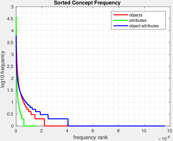
Figure 1: Object (red) and attributes (green) in the VG dataset [11] follow a long tail distribution. Object paired with attributes (blue) much more so.

To validate our approach, we have tested it on the Standford-40 Action dataset [26]. It contains 9532 images with a diverse set of of 40 different action classes, 4000 images for training and the rest for testing. In addition we test our method on the recently introduced HICO [4] dataset, with 47774 images and 600 (not all mutually exclusive) action classes. Following are some technical details, followed by experiments checking various aspects of the method.

As a baseline for purely-visual categorization, we train and test several baseline approaches using feature combinations from various sources: (1) The global average pooling of the VGG-GAP network [27] (2) the output of the 2-before last fully connected layer (termed fc6) from VGG-16 [25] and (3) The pool-5 features from the penultimate layer of ResNet-151 [10]. The feature dimensions are 1024, 4096 and 2048, respectively. In all cases, we train a linear SVM [7] in a one-versus-all manner on $\ell_{2}$ normalized features, or the $\ell_{2}$ normalized concatenation of $\ell_{2}$ features in case of using several feature types. To assign GloVe [20] vectors to object names or attributes, we use the pre-trained model on the Common-Crawl (42B) corpus, which contains a vocabulary of 1.9M words. We break up phrases into their words and assign to them their mean GloVe vector. We discard a few words which are not found in the corpus at all (e.g., “ossicones”).

Figure 2: (blue) The magnitude of weights assigned to different concepts is small for very common (since they are not discriminative) or very rare concepts (since they are harder to learn). The smoothed (red) dots show the moving average of the weight with a window size of 50 concepts, to better show the trend in magnitude.

IV-A Visual vs Concept features

	Stanford-40[26](precision)
Method \ Features	G	G+V	G+V+R
Direct	75.31	78.78	82.97
Concept(Obj)	74.02	77.46	81.27
Concept(Attr)	74.22	77.26	81.07
Concept(Obj-Attr)	38.38	33.88	34.74
Concept(Obj)+Direct	75.31	78.81	83.12
Other Works	80.81 [8]

HICO[4](mAP)
G	G+V	G+V+R
24.96	28.13	31.49
24.4	26.5	29.6
23.9	26.12	28.85
38.38	33.88	34.74
25.06	28.21	31.54
29.4⋆ / 36.1†[16]

TABLE II: Classification accuracy/mAp using direct visual features extracted directly from images (Direct) vs. proposed method (Concept($\cdot$)) for concatenations of various feature types. G: Global-Average-Pooling layer from [27]. V: fc6 from VGG-16 [25]. R: pool5 (penultimate layer) from ResNet-151[10]. Describing images by their set of semantic constituents performs similarly to learning the direct appearance of the classes. The words in brackets specify the types of concepts used (objects/attributes/both). Concept(Obj)+Direct: a weighted combination of the output scores. Rare concepts such as paired object and attributes perform poorly. $\star$: fine-tuned the VGG-16 network. $\dagger$: used detected person bounding boxes; we use the entire image only.

Training and testing by using the visual features is straightforward. For the concept features, we train concept detectors on both the objects and object attributes of the VG dataset. Directly using these in their raw form is infeasible as explained in Sec. III-C. To reduce the number of classes, we normalize each object name beforehand. The object name can be either a single word, such as “dog”, or a phrase, such as “a baseball bat”. To normalize the names, we remove stop-words, such as “the”,”her”,”is”,”a”, as well as punctuation marks. We turn plural words into their singular form. We avoid lemmatizing words since we found that this slightly hinders performance, for example, the word “building” usually refers to the structure and has a different meaning if turned to “build” by lemmatization. Following this process we are left with 66,390 unique object names. They are distributed unevenly, the most common being “man”,”sky”,”ground”,”tree”, etc. We remove all objects with less than 10 images containing them in the dataset, leaving us with 6,063 total object names. We do the same for object attributes: we treat attributes regardless of the object type (e.g, “small dog” and “small tree” are both mapped to “small”), as the number of common object-attribute pairs is much smaller than the number of attributes. Note that the stop-word list for attributes is slightly different, as “white”, a common word in the dataset, is not a noun, but is a proper attribute. We are left with 1740 attributes appearing at least 10 times in the dataset. See Fig. 1 for a visualization of the distribution of the object and attribute frequency. Specifically, one can see that for object-attribute pairs the long-tail distribution is much more accentuated, making them a bad candidate for concepts to learn as features for our target task.

We train classifiers using the detected objects, attributes and object-attributes pairs, as described in sections III-B and III-C. Please refer to Table II for a comparison of the direct-visual results to our method. Except for the attribute-object concepts, we see that the concept based classification does nearly as well as the direct visual-based method, where the addition of ResNet-151 [10] clearly improves results. Combining the predictions from the direct and concept-based (object) predictions and using the ResNet features along with the other representations achieves an improved 83.12% on Stanford-40 [26]. On the recent HICO [4] dataset we obtain a mean average precision of 31.54%. [16] obtain higher results (36.1%) by fusing detected person bounding-boxes with global image context and using a weighted loss.

IV-B Describing Actions using Concepts

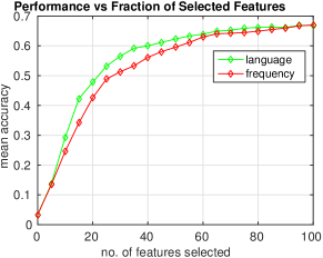
Figure 3: Classification accuracy by selecting the first $k$ concepts according to concept frequency (red) vs. semantic relatedness (green). Semantically related concepts outperform those selected via frequency when using a small number of features.

For each target class, the learned classifier assigns a weight for each of the concepts. Examining this weight vector reveals the concepts deemed most relevant by the classifier. Recall that the weight vector of each learned classifier for class $j$ is $\omega_{j}\in\mathbb{R}^{N}$ ($N$ is the number of target concepts). We checked if the highest-weighted concepts carry semantic meaning with respect to the target classes as follows: for each target class $j\in L$ ($L$ being the set of target classes in $\mathcal{F}$) we sort the values of the learned weight-vector $\omega_{j}$ in descending order, and list the concepts corresponding to the obtained ranking. Table I shows ten arbitrarily chosen classes from the Stanford-40 Actions [26] dataset, with the top 5 ranked object-concepts according to the respective weight-vector. In most cases, the classes are semantically meaningful. However, in some classes we see unexpected concepts, such as holding_an_umbrella$\rightarrow$handbag. This points to a likely bias in the Stanford-40 dataset, such as that many of the subjects holding umbrellas in the training images also carry handbags, which was indeed found to be the case by examining the training images for this class.

An interesting comparison is the concepts differentiating between related classes. For example, the top 5 ranked keywords for the class “feeding a horse” are (“mane”, “left_ear”, “hay”, “nostril”, “horse”) whereas for “riding a horse” they are (“saddle”, “horse”, “rider”, “hoof”, “jockey”). While “horse” is predictably common to both, other words are indeed strongly related to one of the classes but not the other, for example, “hay” for feeding vs “jockey”, “saddle” for riding.

IV-C Concept Visualization

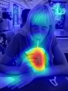
(a)

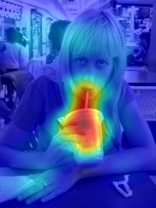
(b)

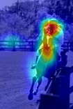
(c)

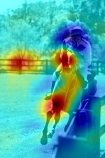
(d)

(e)

(f)

Figure 4: Forcing the method to explain the wrong class: the proposed method detects action classes by a weighted sum of learned concepts. We visualize (using [27]) highlighted regions contributing to the strongest concepts related to the correct vs the incorrect class . The correct(incorrect) pairs are : (a,b) drinking (smoking) (c,d) riding a horse (feeding a horse) (e,f) taking photos (phoning). When forced to explain the image differently, the method highlights different concepts, relevant to the desired class: “smoking” shifts focus to the immediate mouth area while “drinking” on the cup. “feeding a horse” focuses on the head and lower body of the horse, “riding a horse” on the rider. “taking photos” focuses on the cameras, “phoning” on the hand-held phone.

To test what features contribute most to the classification result, we use the Class-Activation-Map (CAM) [27]. This method allows to visualize what image regions contributed the most to the score of each class. We can do this for the version of our method which uses only the VGG-GAP features, as the method requires a specific architecture to re-project classification scores to the image (see [27] for details). We visualize the average CAMs of the top-5 ranked keywords for different classes (as in the above section). We do this for two target classes for each image, one correct class and the other incorrect, to explain what image regions drive the method to decide on the image class. See Fig. 4. When the method is “forced” to explain the riding image as “feeding a horse”, we see negative weights on the rider and strong positive weights on the lower part of the horse, whereas examining the regions contributing to “riding a horse” gives a high weight to the region containing the jockey.

IV-D Distribution of Weights

We have also examined the overall statistics of the learned weight vectors. For a single weight vector $\omega$, we define:

$$abs(\omega) = [\left|\omega_{1}\right|,\left|\omega_{2}\right|,\dots,\left|\omega_{N}\right|]$$ (8)

$$\bar{\omega} = \frac{1}{N}\sum_{j=1}^{L}abs(\omega_{j})$$ (9)

i.e, $\bar{\omega}$ is the mean of $abs(\omega)$ for all classifiers of the target classes. Fig. 2 displays these mean absolute weights assigned to object concepts, ordered by their frequency in VG. Not surprisingly, the first few tens of concepts have low-magnitude weights, as they are too common to be discriminative. The next few hundreds of concepts exhibit higher weights, and finally, weights become lower with diminished frequency. This can be explained due to such concepts having weaker classifiers as they have fewer positive examples, making them less reliable. A similar trend was observed when examining attributes.

IV-E Feature Selection by Semantic Relatedness

Section IV-B provided a qualitative measure of the keywords found by the proposed method. Here, we take on a different approach, which is selecting concepts by a relatedness measure to the target classes, and measuring how well training using these concepts alone compares with choosing the top-k most common concepts. To do so, we measure their mean “importance”. As described in Section III-C we assign to each concept $c\in C$ a GloVe [20] representation $V_{c}$. Similarly, we assign a vector $V_{p}$ to each target class $p\in L$ according to its name; for instance, “riding a horse” is assigned the mean of the vectors of the words “ride” and “horse”. Then, for each class $p$ we rank the $V_{c}$ vectors according to their euclidean distance from $V_{p}$ in increasing order. This induces a per-class order $\sigma_{p}=exc_{p,1}\dots c_{p,2}$, which is a permutation of $1...\left|C\right|$, such that $c_{p,i}$ is the ranking of $c_{i}$ in the ordering induced by $p$. We use this to define the new mean rank $r(c)$ of each concept:

$$r(c) = {\displaystyle\sum_{p=1}^{L}}\exp(-\sigma_{p}(c))$$ (10)

Now, we test the predictive ability of concepts chosen from $C$ according to two orderings. The first is the frequency of $c$, in ascending order, and the second is the sorted values (descending) of $r(c)$ as defined in Eqn. 10. We select the first $k$ concepts for the first $k\in(0,5,10,15,\dots,100)$ features ($k=0$ for chance performance). For a small amount of features, e.g., $k=15$, the concepts chosen according to $r(c)$ outperform those chosen according to frequency by a large margin, i.e, 42.2 vs 34.2 respectively.

V Conclusions & Future Work

We have presented a method which learns to recognize actions in images by describing them as a weighted sum of detected concepts (objects and object attributes). The method utilizes the annotations in the VG dataset to learn a broad range of concepts, which are then used to recognize action in still images. We are able to improve on classification performance versus of a strong baseline which uses purely visual features, as well as provide a visual and semantic explanation of the classifier’s decisions. In the future we intend to broaden our work to capture object relationships, which are very important to action-classification as well.

References

- [1] David Arthur and Sergei Vassilvitskii. k-means++: The advantages of careful seeding. In Proceedings of the eighteenth annual ACM-SIAM symposium on Discrete algorithms, pages 1027–1035. Society for Industrial and Applied Mathematics, 2007.
- [2] David Bau, Bolei Zhou, Aditya Khosla, Aude Oliva, and Antonio Torralba. Network Dissection: Quantifying Interpretability of Deep Visual Representations. arXiv preprint arXiv:1704.05796, 2017.
- [3] Hakan Bilen and Andrea Vedaldi. Weakly Supervised Deep Detection Networks. arXiv preprint arXiv:1511.02853, 2015.
- [4] Yu-Wei Chao, Zhan Wang, Yugeng He, Jiaxuan Wang, and Jia Deng. HICO: A Benchmark for Recognizing Human-Object Interactions in Images. In Proceedings of the IEEE International Conference on Computer Vision, pages 1017–1025, 2015.
- [5] Ramazan Gokberk Cinbis, Jakob Verbeek, and Cordelia Schmid. Weakly Supervised Object Localization with Multi-fold Multiple Instance Learning. arXiv preprint arXiv:1503.00949, 2015.
- [6] Mark Everingham, Luc Van Gool, Christopher KI Williams, John Winn, and Andrew Zisserman. The pascal visual object classes (voc) challenge. International journal of computer vision, 88(2):303–338, 2010.
- [7] Rong-En Fan, Kai-Wei Chang, Cho-Jui Hsieh, Xiang-Rui Wang, and Chih-Jen Lin. LIBLINEAR: A Library for Large Linear Classification. Journal of Machine Learning Research, 9:1871–1874, 2008.
- [8] Bin-Bin Gao, Xiu-Shen Wei, Jianxin Wu, and Weiyao Lin. Deep spatial pyramid: The devil is once again in the details. arXiv preprint arXiv:1504.05277, 2015.
- [9] Jiyang Gao, Chen Sun, and Ram Nevatia. ACD: Action Concept Discovery from Image-Sentence Corpora. arXiv preprint arXiv:1604.04784, 2016.
- [10] Kaiming He, Xiangyu Zhang, Shaoqing Ren, and Jian Sun. Deep Residual Learning for Image Recognition. arXiv preprint arXiv:1512.03385, 2015.
- [11] Ranjay Krishna, Yuke Zhu, Oliver Groth, Justin Johnson, Kenji Hata, Joshua Kravitz, Stephanie Chen, Yannis Kalantidis, Li-Jia Li, David A. Shamma, Michael S. Bernstein, and Fei-Fei Li. Visual Genome: Connecting Language and Vision Using Crowdsourced Dense Image Annotations. CoRR, abs/1602.07332, 2016.
- [12] Christoph H Lampert, Hannes Nickisch, and Stefan Harmeling. Learning to detect unseen object classes by between-class attribute transfer. In Computer Vision and Pattern Recognition, 2009. CVPR 2009. IEEE Conference on, pages 951–958. IEEE, 2009.
- [13] Li-Jia Li, Hao Su, Li Fei-Fei, and Eric P Xing. Object bank: A high-level image representation for scene classification & semantic feature sparsification. In Advances in neural information processing systems, pages 1378–1386, 2010.
- [14] Xirong Li, Shuai Liao, Weiyu Lan, Xiaoyong Du, and Gang Yang. Zero-shot image tagging by hierarchical semantic embedding. In Proceedings of the 38th International ACM SIGIR Conference on Research and Development in Information Retrieval, pages 879–882. ACM, 2015.
- [15] Tsung-Yi Lin, Michael Maire, Serge Belongie, James Hays, Pietro Perona, Deva Ramanan, Piotr Dollár, and C Lawrence Zitnick. Microsoft coco: Common objects in context. In Computer Vision–ECCV 2014, pages 740–755. Springer, 2014.
- [16] Arun Mallya and Svetlana Lazebnik. Learning Models for Actions and Person-Object Interactions with Transfer to Question Answering. arXiv preprint arXiv:1604.04808, 2016.
- [17] George A Miller. WordNet: a lexical database for English. Communications of the ACM, 38(11):39–41, 1995.
- [18] Mohammad Norouzi, Tomas Mikolov, Samy Bengio, Yoram Singer, Jonathon Shlens, Andrea Frome, Greg S Corrado, and Jeffrey Dean. Zero-shot learning by convex combination of semantic embeddings. arXiv preprint arXiv:1312.5650, 2013.
- [19] Deepak Pathak, Philipp Krahenbuhl, and Trevor Darrell. Constrained convolutional neural networks for weakly supervised segmentation. In Proceedings of the IEEE International Conference on Computer Vision, pages 1796–1804, 2015.
- [20] Jeffrey Pennington, Richard Socher, and Christopher D Manning. Glove: Global Vectors for Word Representation. In EMNLP, volume 14, pages 1532–1543, 2014.
- [21] Vignesh Ramanathan, Congcong Li, Jia Deng, Wei Han, Zhen Li, Kunlong Gu, Yang Song, Samy Bengio, Chuck Rossenberg, and Li Fei-Fei. Learning semantic relationships for better action retrieval in images. In Computer Vision and Pattern Recognition (CVPR), 2015 IEEE Conference on, pages 1100–1109. IEEE, 2015.
- [22] Olga Russakovsky, Jia Deng, Hao Su, Jonathan Krause, Sanjeev Satheesh, Sean Ma, Zhiheng Huang, Andrej Karpathy, Aditya Khosla, Michael Bernstein, Alexander C. Berg, and Li Fei-Fei. ImageNet Large Scale Visual Recognition Challenge. International Journal of Computer Vision (IJCV), 115(3):211–252, 2015.
- [23] Sreemanananth Sadanand and Jason J Corso. Action bank: A high-level representation of activity in video. In Computer Vision and Pattern Recognition (CVPR), 2012 IEEE Conference on, pages 1234–1241. IEEE, 2012.
- [24] Ruslan Salakhutdinov, Antonio Torralba, and Josh Tenenbaum. Learning to share visual appearance for multiclass object detection. In Computer Vision and Pattern Recognition (CVPR), 2011 IEEE Conference on, pages 1481–1488. IEEE, 2011.
- [25] Karen Simonyan and Andrew Zisserman. Very deep convolutional networks for large-scale image recognition. arXiv preprint arXiv:1409.1556, 2014.
- [26] Bangpeng Yao, Xiaoye Jiang, Aditya Khosla, Andy Lai Lin, Leonidas Guibas, and Li Fei-Fei. Human action recognition by learning bases of action attributes and parts. In Computer Vision (ICCV), 2011 IEEE International Conference on, pages 1331–1338. IEEE, 2011.
- [27] Bolei Zhou, Aditya Khosla, Agata Lapedriza, Aude Oliva, and Antonio Torralba. Learning Deep Features for Discriminative Localization. arXiv preprint arXiv:1512.04150, 2015.
- [28] Xiangxin Zhu, Dragomir Anguelov, and Deva Ramanan. Capturing long-tail distributions of object subcategories. In Proceedings of the IEEE Conference on Computer Vision and Pattern Recognition, pages 915–922, 2014.