A matrix method for fractional Sturm-Liouville problems on bounded domain.

Abstract

A matrix method for the solution of direct fractional Sturm-Liouville problems on bounded domain is proposed where the fractional derivative is defined in the Riesz sense. The scheme is based on the application of the Galerkin spectral method of orthogonal polynomials. The order of convergence of the eigenvalue approximations with respect to the matrix size is studied. Some numerical examples that confirm the theory and prove the competitiveness of the approach are finally presented.

1 Introduction

This paper concerns the numerical approximation of the eigenvalues of a time-independent one-dimensional fractional Schroedinger equation defined on a bounded interval which, without loss of generality, we assume to be $(-1,1).$ This problem has several important applications. Among them we cite quantum mechanics with a Feynman path integral over Lévy trajectories, [21, 22]. Many other applications appear in mathematical physics, biology and finance.

In more details, we shall consider the following eigenvalue problem

$$\left(-\Delta\right)^{{\alpha/2}}y(x)+q(x)y(x)=\lambda\,y(x),\qquad x\in D\equiv(-1,1),$$ (1)

$$\qquad\qquad y(x)=0\quad\mbox{for each \,\,}x\in{\mathbb{R}}\setminus D,$$ (2)

where $\lambda$ and $y$ are an eigenvalue and a corresponding eigenfunction, respectively, $q$ represents the potential, and, for ${\alpha}\in(0,2),$ the fractional Laplace operator (or quantum Riesz derivative) is defined as

$$\left(-\Delta\right)^{{\alpha/2}}y(x)\equiv\frac{1}{\eta({\alpha})}\lim_{\varepsilon\rightarrow 0^{+}}\int_{{\mathbb{R}}\setminus(-\varepsilon,\varepsilon)}\frac{y(x)-y(x-t)}{|t|^{1+{\alpha}}}dt,$$ (3)

with

$$\eta({\alpha})=-\frac{\pi^{1/2}{\Gamma}(-{\alpha/2})}{2^{\alpha}{\Gamma}((1+{\alpha})/2)}=-2{\Gamma}(-{\alpha})\cos({\alpha}\pi/2).$$

Indeed several definitions of the fractional Laplacian can be found in the literature which are equivalent to (3) if $y$ and/or $\alpha$ verify suitable hypotheses (see, for instance, [20, 23, 24, 28]). One of them is given by the pseudo-differential operator with symbol $|\omega|^{\alpha}$, i.e.

$$\left(-\Delta\right)^{{\alpha/2}}y(x)={\cal F}^{-1}\left\{|\omega|^{\alpha}\hat{y}(\omega);x\right\}=\frac{1}{2\pi}\int_{-\infty}^{+\infty}|\omega|^{\alpha}e^{i\omega x}\hat{y}(\omega)\>d\omega,$$

where $\hat{y}$ is the Fourier transform of $y.$ It is known that this definition is equivalent to (3) if $y\in L^{s}({\mathbb{R}})$ with $s\in[1,2],$ [20].
Alternatively, if ${\alpha}\in(0,2)\setminus\left\{1\right\}$ then (3) can be written as

$$\left(-\Delta\right)^{{\alpha/2}}y(x)=\frac{\sin({\alpha}\pi/2)}{\sin({\alpha}\pi)}\,\frac{d^{n}}{dx^{n}}I^{(n-{\alpha})}y(x),$$ (4)

where $n=\lceil{\alpha}\rceil$ and

$$I^{(n-{\alpha})}y(x) = \frac{1}{\Gamma(n-{\alpha})}\int_{-\infty}^{+\infty}\left(\mbox{sign}(x-t)\right)^{n}|x-t|^{n-{\alpha}-1}y(t)dt$$

$$= \int_{-\infty}^{x}\frac{(x-t)^{n-{\alpha}-1}}{\Gamma(n-{\alpha})}y(t)dt+(-1)^{n}\int_{x}^{+\infty}\frac{(t-x)^{n-{\alpha}-1}}{\Gamma(n-{\alpha})}y(t)dt$$

$$\equiv I_{+}^{(n-{\alpha})}y(x)+(-1)^{n}I_{-}^{(n-{\alpha})}y(x).$$

Here, $I_{\pm}^{(n-{\alpha})}$ are the left- and right-sided Riemann-Liouville fractional integrals (sometimes called Weyl integrals) of order $n-{\alpha}.$
Justified by passage to the limit ${\alpha}\nearrow n,$ $I_{\pm}^{(0)}$ are defined as the identity operator and, consequently, $\left(-\Delta\right)^{{\alpha/2}}$ is set equal to $-\frac{d^{2}}{dx^{2}}$ for ${\alpha}=2,$ [23]. This implies that, for such value of ${\alpha},$ (1)-(2) reduces to the classical Sturm-Liouville problem in normal form with Dirichlet boundary conditions at both ends.

Concerning the special case of $q(x)\equiv 0$ in $D,$ sometimes referred to as the infinite potential well problem, it is known that the eigenvalues of (1)-(2) form an infinite sequence tending to infinity. More precisely, if we denote them with $\lambda_{k}$ then it is known that $0<\lambda_{0}<\lambda_{1}\leq\lambda_{2}\leq\lambda_{3}\leq\ldots$ and that the corresponding eigenfunctions, say $y_{k},$ form a complete orthonormal set in $L^{2}(D),$ [3, 6]. Regarding the simplicity of the eigenvalues in [19], see also the references therein, it was proved that this property is surely verified if ${\alpha}\in[1,2]$ and it was conjectured that indeed it holds for every ${\alpha}\in(0,2].$ Moreover, in the same paper, the following asymptotic law

$$\lambda_{k}=\left(\frac{(k+1)\pi}{2}-\frac{(2-{\alpha})\pi}{8}\right)^{\alpha}+O\left(\frac{1}{k+1}\right)$$ (5)

was determined (please observe that we number the eigenvalues starting from $k=0$ instead of $k=1$ as done in [19]). It must be said that an asymptotic growth like $((k+1)\pi/2)^{\alpha}$ was already proved in [8, 9].
Now if $q\in L^{2}(D)$ then for the classical problem with ${\alpha}=2$ it is known that

$$\lambda_{k}(q)\approx\lambda_{k}(0)+\bar{q},\qquad\bar{q}=\frac{1}{2}\int_{-1}^{1}q(x)dx,\qquad k\gg 0,$$ (6)

where $\lambda_{k}(q)$ and $\lambda_{k}(0)$ are the eigenvalues of index $k$ for the problems with potential $q$ and zero potential in $D,$ respectively. More precisely, the residuals $\delta_{k}=\lambda_{k}(q)-\lambda_{k}(0)-\bar{q},$ $k\in{\mathbb{N}}_{0},$ depend on $q-\bar{q}$ and constitute a square-summable sequence. In addition, their rate of decrease is connected to the smoothness of $q$ over $[-1,1],$ [27]. It is reasonable to assume that (6) holds true for each $\alpha\in(0,2]$ under the same hypothesis for $q.$

In the literature, the numerical schemes currently availables for the problem under consideration belong to the family of so-called matrix methods, namely methods that discretize the eigenvalue problem for the differential operator as an ordinary or a generalized matrix eigenvalue one. In particular, a number of finite difference schemes that constitute a generalization of the classical three-point method (or discrete Laplacian in 1D) are available. This is the case, for example, of the method proposed independently by Ortigueira and by Zoia et.al. in [25, 35] and of the WSGD method (acronym for Weighted and Shifted Grünwald Difference) studied in [31]. In the former case, the discrete fractional Laplacian is represented by the symmetric Toeplitz matrix $T_{\alpha}$ with symbol $(2(1-\cos\theta))^{\alpha/2}$ (note that $2(1-\cos\theta)$ is the symbol associated to $T=\mbox{tridiag}(-1,2,-1)).$ The WSGD method, instead, provides an approximation of the left- or the right-sided Riemann-Liouville fractional derivatives by using a suitable combination of the Grünwald and the shifted Grünwald difference schemes. In both the previous cases, in [7, 31] it was proved that if $y$ is sufficiently regular over ${\mathbb{R}}$ and if $\alpha\in(1,2]$ then the error in the approximation of $\left(-\Delta\right)^{\alpha/2}y(x_{n})$ behaves like $O(h^{2}),$ where $x_{n}$ and $h$ represent a meshpoint and the stepsize, respectively. Unfortunately, the eigenfunctions of (1)-(2) are not smooth in proximity of the boundary of $D.$ For the problem with zero potential in $D,$ in fact, it is known that there exist suitable constants $C_{1},\,C_{2},\,C_{3}$ and $\theta$ such that

$$y(x)\approx\left\{\begin{array}[]{ll}C_{1}(1+x)^{\alpha/2}&\mbox{for }x\mbox{ close to }-1,\\ C_{2}(1-x)^{\alpha/2}&\mbox{for }x\mbox{ close to }1,\\ C_{3}\sin(\lambda^{1/{\alpha}}x+\theta)&\mbox{for }x\in D\mbox{ away from the boundary,}\end{array}\right.$$ (7)

see, for instance, [19] and [18, Example 1]. We expect that if $q\in L^{2}(D)$ and if $\|q-\bar{q}\|_{2}$ is not too large then the eigenfunctions have a similar behavior. The lack of regularity near the boundaries of the domain is a peculiarity of the solution of differential problems that involve fractional operators and, in addition to the nonlocality of the latters, it represents a further important source of difficulties for their numerical treatment. With reference to the matrix methods previously mentioned, such behavior of $y$ determines an order reduction in the approximation of its fractional Laplacian and consequently in the resulting numerical eigenvalues. Alternative matrix methods are those proposed recently in [5, 10, 15]. In particular, the method in [5] is based on finite element approximations and it can be applied to problems in a generic dimension $d\geq 1,$ the approach considered in [10] is that of using suitable quadratures for the approximation of the integral in (3) and, finally, in [15] a Control Volume Function approximation with Radial Basis Function interpolation is proposed. All these schemes, however, appear to be of the first order, namely the error in the approximation of the eigenvalues decreases like $N^{-1}$ where $N$ is the matrix size.

In this paper, we propose a matrix method based on the Galerkin spectral schemes named method of orthogonal polynomials in [26] (see also the references therein). Indeed, the principal idea has been recently presented in [11] which concerns the eigenvalue problem for the fractional Laplace operator in the unit ball of dimension $d\geq 1$ (so the potential is identically zero in $D$). In such paper, it is proved that the eigenvalues provided by the matrix method with matrices of order $N,$ say $\lambda_{k}^{(N)},$ are such that $\lambda_{k}\leq\lambda_{k}^{(N)},$ for each $k<N.$ This is done by using the standard Rayleigh-Ritz variational method. In addition, the Aronszajn method of intermediate problems, see e.g. [4], is used for getting a lower bound for the eigenvalues. The aim pursued in [11] is that of proving that if $1\leq d\leq 9$ and $\alpha=1$ or if $1\leq d\leq 2$ and $\alpha\in(0,2]$ then the eigenfunctions corresponding to $\lambda_{1}$ are antisymmetric. In this paper, we are going to study such matrix method for $d=1$ from a numerical point of view. More precisely, differently with respect to what has been done in [11], we shall consider a generic potential $q\in L^{2}(D)$ and we will study the order of convergence of $|\lambda_{k}-\lambda_{k}^{(N)}|$ with respect to $N.$ Before proceeding, it must be said that the application of the method of orthogonal polynomials to fractional eigenvalue problems has been recently considered also in [33, 34] which however concern different fractional operators. For example, one of the generalization of the differential term $\frac{d}{dx}\left[p(x)\frac{d}{dx}\right]$ of the classical Sturm-Liouville operator considered in [33] (see also [17]) is given by $\,{}_{~{}x}^{RL}D_{1}^{{\alpha/2}}\left[p(x)\,_{-1}^{~{}C}D_{x}^{{\alpha/2}}\right].$ Here ${}_{~{}x}^{RL}D_{1}^{{\alpha/2}}$ and ${}_{-1}^{~{}C}D_{x}^{{\alpha/2}}$ are the right-sided Riemann-Liouville derivative of order ${\alpha/2},$ and the left-sided Caputo derivative of the same order, respectively.

The paper is organized as follows. In Section 2 we introduce the approach based on the spectral method of orthogonal polynomials. In Section 3 we derive the generalized matrix eigenvalue problem that discretize (1)-(2). Moreover, we describe how we have handled a generic potential $q\in L^{2}(D)$ and we study the behavior of the entries in the resulting coefficient matrices. Section 4 is devoted to the analysis of the error in the eigenvalue approximations while Section 5 to the study of the conditioning of the numerical eigenvalues with respect to a perturbation of the potential. Finally, in Section 6 we report the results of several numerical examples that confirm the theory and prove the competitiveness of our method.

2 Spectral method of orthogonal polynomials

By virtue of (7), we consider the following expansion of an eigenfunction of (1)-(2)

$$y(x)=(1-x^{2})_{+}^{{\alpha/2}}\sum_{n=0}^{\infty}c_{n}P_{n}^{({\alpha/2},{\alpha/2})}(x).$$ (8)

Here $a_{+}=\max(a,0)$ and, for $\beta,\gamma>-1,$ $\left\{P_{n}^{(\beta,\gamma)}\right\}_{n\in{\mathbb{N}}_{0}}$ is the sequence of orthogonal Jacobi polynomials in $L^{2}(D,\omega)$ with weighting function $\omega(x)=(1-x)^{\beta}(1+x)^{\gamma},$ i.e. $\langle P_{n}^{(\beta,\gamma)},P_{m}^{(\beta,\gamma)}\rangle_{\beta,\gamma}=0$ for each $n\neq m$ being

$$\langle f,g\rangle_{\beta,\gamma}\equiv\int_{-1}^{1}(1-x)^{\beta}(1+x)^{\gamma}f(x)\>g(x)\>dx,\quad f,g\in L^{2}(D,\omega).$$ (9)

In particular, the following normalization

$$P_{n}^{(\beta,\gamma)}(1)=1$$

will be used for such polynomials. If $\beta=\gamma$ then we shall use the simpler notation

$$P_{n}^{(\beta)}\equiv P_{n}^{(\beta,\beta)},\qquad\langle\cdot,\cdot\rangle_{\beta}\equiv\langle\cdot,\cdot\rangle_{\beta,\beta}.$$ (10)

As we are going to show in Theorem 2.1, the expansion in (8) is favorable since

$$\left(-\Delta\right)^{{\alpha/2}}\left((1-x^{2})_{+}^{{\alpha/2}}P_{n}^{({\alpha/2})}(x)\right)\propto P_{n}^{({\alpha/2})}(x)\quad\mbox{for each }x\in(-1,1).$$

Before this important result, for later convenience, we recall a list of known properties of the Jacobi polynomials revised according to the normalization that we have considered:

1. $\sigma_{n}\equiv\langle P_{n}^{({\alpha/2})},P_{n}^{({\alpha/2})}\rangle_{{\alpha/2}}=\frac{2^{{\alpha}+1}{\Gamma}(n+1){\Gamma}^{2}({\alpha/2}+1)}{(2n+{\alpha}+1){\Gamma}(n+{\alpha}+1)};$

2. if $n$ is even then $P_{n}^{({\alpha/2})}(x)=P_{n/2}^{({\alpha/2},-1/2)}(2x^{2}-1);$

3. if $n$ is odd then $P_{n}^{({\alpha/2})}(x)=xP_{(n-1)/2}^{({\alpha/2},1/2)}(2x^{2}-1);$

4. for each $\beta,\gamma,\sigma>-1,$ [13, 16.4 formula (17)],

   $$\langle P_{r}^{(\beta,\gamma)},P_{s}^{(\sigma,\gamma)}\rangle_{\beta+\sigma,\gamma}=$$

   $$\frac{(-1)^{r-s}\,2^{\gamma+\beta+\sigma+1}\,{\Gamma}(\beta+\sigma+1)\,{\Gamma}(\gamma+r+s+1){\Gamma}(\beta+1){\Gamma}(\sigma+1)}{{\Gamma}(\beta+r-s+1)\,{\Gamma}(\sigma+s-r+1)\,{\Gamma}(\gamma+\beta+\sigma+r+s+2)};$$

5. the polynomials $P_{n}^{({\alpha/2})}$ verify the following recurrence relation

   $$P_{-1}^{({\alpha/2})}(x) \equiv 0,$$

   $$P_{0}^{({\alpha/2})}(x) \equiv 1,$$ (11)

   $$P_{n+1}^{({\alpha/2})}(x) = \frac{2n+1+{\alpha}}{n+1+{\alpha}}x\,P_{n}^{({\alpha/2})}(x)-\frac{n}{n+1+{\alpha}}P_{n-1}^{({\alpha/2})}(x)$$ (12)

   $$\equiv \zeta_{n,1}xP_{n}^{({\alpha/2})}(x)-\zeta_{n,0}P_{n-1}^{({\alpha/2})}(x),\quad n\geq 0;$$ (13)

6. $P_{n}^{({\alpha/2})}(x)=\frac{\Gamma({\alpha}+1)\Gamma(n+1)}{\Gamma(n+{\alpha}+1)}\,C_{n}^{({\alpha/2}+1/2)}(x),$ where $C_{n}^{({\alpha/2}+1/2)}$ is the Gegenbauer polynomial of degree $n$ with its usual normalization, [2, 30];

7. $P_{n}^{(\beta,\gamma)}(x)$ coincides with the following Gauss hypergeometric function

   $$P_{n}^{(\beta,\gamma)}(x)=\,_{2}F_{1}\left(-n,n+\beta+\gamma+1;\beta+1;(1-x)/2\right).$$ (14)

The latter property allows to extend the definition of $P_{n}^{(\beta,\gamma)}$ to all $\beta,\gamma\in{\mathbb{R}}$ with $-\beta\notin{\mathbb{N}},$ [30].

We can now prove the following spectral relationship which is fundamental for the development of the method.

Theorem 2.1

If ${\alpha}\in(0,2]$ then for each $n\geq 0$ and each $x\in(-1,1)$

$$\left(-\Delta\right)^{{\alpha/2}}\left((1-x^{2})_{+}^{{\alpha/2}}P_{n}^{({\alpha/2})}(x)\right)=\mu_{n}P_{n}^{({\alpha/2})}(x),$$ (15)

where

$$\mu_{n}=\frac{{\Gamma}(n+{\alpha}+1)}{{\Gamma}(n+1)}.$$ (16)

Proof If ${\alpha}=2$ then $P_{n}^{(1)}(x)=L_{n+1}^{\prime}(x)$ where $L_{n+1}(x)$ is the Legendre polynomial of degree $n+1,$ with a suitable normalization, and $\mu_{n}=(n+2)(n+1).$ It follows that (15)-(16) reduce to the well-known identity

$$-\frac{d^{2}}{dx^{2}}\left((1-x^{2})L_{n+1}^{\prime}(x)\right)=(n+2)(n+1)L_{n+1}^{\prime}(x),\qquad x\in(-1,1).$$

Let’s consider the case ${\alpha}\in(0,2)$ and ${\alpha}\neq 1.$ After some computations, by using (4) and (14), one obtains that (15)-(16) are an application of Theorems 6.2 and 6.3 in [26]. The special value ${\alpha}=1$ follows by continuity.
Alternatively, by virtue of properties P2 and P3, the statement is an application of Theorem 3 in [12] for every ${\alpha}\in(0,2].$ $\Box$

Now, if $y$ satisfies (1)-(2) with eigenvalue $\lambda$ then for each $m\in{\mathbb{N}}_{0}$

$$\langle P_{m}^{({\alpha/2})},\left(-\Delta\right)^{{\alpha/2}}y\rangle_{{\alpha/2}}+\langle P_{m}^{({\alpha/2})},qy\rangle_{{\alpha/2}}=\lambda\langle P_{m}^{({\alpha/2})},y\rangle_{{\alpha/2}},$$ (17)

see (9)-(10). Therefore, from (8) and (15)-(16) one gets that the first term in the previous equation reduces to

$$\langle P_{m}^{({\alpha/2})},\left(-\Delta\right)^{{\alpha/2}}y\rangle_{{\alpha/2}}=\mu_{m}\langle P_{m}^{({\alpha/2})},P_{m}^{({\alpha/2})}\rangle_{{\alpha/2}}c_{m}\equiv a_{m}c_{m}$$

where, see property P1,

$$a_{m}=\mu_{m}\langle P_{m}^{({\alpha/2})},P_{m}^{({\alpha/2})}\rangle_{{\alpha/2}}=\frac{2^{{\alpha}+1}{\Gamma}^{2}({\alpha/2}+1)}{2m+{\alpha}+1}.$$ (18)

Concerning the inner product on the right-hand side of (17), from (8) it follows that

$$\langle P_{m}^{({\alpha/2})},y\rangle_{{\alpha/2}}\equiv\sum_{n=0}^{\infty}b_{mn}c_{n},\qquad b_{mn}\equiv\langle P_{m}^{({\alpha/2})},P_{n}^{({\alpha/2})}\rangle_{{\alpha}}.$$ (19)

It is evident that $b_{mn}=0$ for each $m$ and $n$ such that $m+n$ is odd. Moreover, the application of properties P2–P4 allows to determine the remaining values analytically.
Let us consider the case where $m=2r$ and $n=2s.$ By using property P2, one deduces that

$$b_{mn}=\int_{-1}^{1}(1-x^{2})^{{\alpha}}P_{m}^{({\alpha/2})}(x)P_{n}^{({\alpha/2})}(x)dx$$ (20)

$$=2\int_{0}^{1}(1-x^{2})^{{\alpha}}P_{r}^{({\alpha/2},-1/2)}(2x^{2}-1)P_{s}^{({\alpha/2},-1/2)}(2x^{2}-1)dx$$

$$=\frac{1}{2^{1/2+{\alpha}}}\int_{-1}^{1}(1-t)^{{\alpha}}(1+t)^{-1/2}P_{r}^{({\alpha/2},-1/2)}(t)P_{s}^{({\alpha/2},-1/2)}(t)dt$$

$$=\frac{(-1)^{(m-n)/2}\,{\Gamma}({\alpha}+1)\,{\Gamma}((m+n+1)/2)\,{\Gamma}^{2}({\alpha/2}+1)}{{\Gamma}(({\alpha}-m+n)/2+1)\,{\Gamma}(({\alpha}-n+m)/2+1){\Gamma}((m+n+3)/2+{\alpha})}.$$

In particular, the last equality follows from property P4 with $\gamma=-1/2,$ $\beta=\sigma={\alpha/2},$ $r=m/2,$ and $s=n/2.$ It must be said that the previous formula was already determined in [12], with suitable changes in the notation and by considering the different normalization of the Jacobi polynomials.
Now (20) holds true also in the case where $m$ and $n$ are odd, i.e. $m=2r+1$ and $n=2s+1.$ In fact, from property P3, we get

$$b_{mn} = 2\int_{0}^{1}(1-x^{2})^{{\alpha}}x^{2}P_{r}^{({\alpha/2},1/2)}(2x^{2}-1)P_{s}^{({\alpha/2},1/2)}(2x^{2}-1)dx$$

$$= \frac{1}{2^{3/2+{\alpha}}}\int_{-1}^{1}(1-t)^{{\alpha}}(1+t)^{1/2}P_{r}^{({\alpha/2},1/2)}(t)P_{s}^{({\alpha/2},1/2)}(t)dt$$

which one can verify to be equal to the right-hand side of (20) by using property P4 with $\gamma=1/2,$ $\beta=\sigma={\alpha/2},$ $r=(m-1)/2,$ and $s=(n-1)/2.$

We observe that the application of Euler’s reflection formula ${\Gamma}(1-z){\Gamma}(z)=\pi/\sin(\pi z),$ see also [25, eq.(4.21)-(4-23)], allows to get that if $m+n$ is even then

$$\frac{(-1)^{(m-n)/2}}{{\Gamma}(({\alpha}-m+n)/2+1)\,{\Gamma}(({\alpha}-n+m)/2+1)}=-\frac{\sin(\pi{\alpha/2})}{\pi}\,\frac{{\Gamma}\left(\left|\frac{n-m}{2}\right|-\frac{{\alpha}}{2}\right)}{{\Gamma}\left(\left|\frac{n-m}{2}\right|+\frac{{\alpha}}{2}+1\right)}.$$

This implies that the coefficient $b_{mn}$ in (20) can be written as

$$b_{mn}=\theta_{\alpha}h_{m+n}t_{|n-m|}$$ (21)

where

$$\theta_{\alpha} = -\frac{\sin(\pi{\alpha/2}){\Gamma}({\alpha}+1)\,{\Gamma}^{2}({\alpha/2}+1)}{\pi},$$

$$h_{m+n} = \frac{{\Gamma}((m+n+1)/2)}{{\Gamma}((m+n+3)/2+{\alpha})},$$ (22)

$$t_{|n-m|} = \frac{{\Gamma}\left(\left|\frac{n-m}{2}\right|-\frac{{\alpha}}{2}\right)}{{\Gamma}\left(\left|\frac{n-m}{2}\right|+\frac{{\alpha}}{2}+1\right)}.$$ (23)

3 Numerical scheme

In order to get a numerical method for the approximation of the eigenvalues and of the eigenfunctions of the fractional Sturm-Liouville problem, we truncate the series in (8), i.e. we look for an approximation of $y$ of the form

$$y(x)\approx y^{(N)}(x)=(1-x^{2})_{+}^{{\alpha/2}}\sum_{n=0}^{N-1}\xi_{n,N}P_{n}^{({\alpha/2})}(x)$$ (24)

where the coefficients $\xi_{n,N}$ are determined by imposing that (17) holds true for $m=0,\ldots,N-1$ with $y$ and $\lambda$ replaced by $y^{(N)}$ and $\lambda^{(N)}$ respectively. This leads to a generalized matrix eigenvalue problem of the form

$$\left(A_{N}+Q_{N}\right)\mbox{\boldmath$\xi$}_{N}=\lambda^{(N)}B_{N}\mbox{\boldmath$\xi$}_{N},$$ (25)

where $\mbox{\boldmath$\xi$}_{N}=\left(\xi_{0,N},\xi_{1,N},\ldots,\xi_{N-1,N}\right)^{T}$ and, see (18)-(19),

$$A_{N}=\mbox{diag}\left(a_{0},\ldots,a_{N-1}\right),\qquad B_{N}=\left(b_{mn}\right)_{m,n=0,\ldots,N-1}.$$

Finally, the entries of $Q_{N}$ are given by

$$q_{mn}=\langle P_{m}^{({\alpha/2})},qP_{n}^{({\alpha/2})}\rangle_{{\alpha}}=\int_{-1}^{1}(1-x^{2})^{{\alpha}}q(x)P_{m}^{({\alpha/2})}(x)P_{n}^{({\alpha/2})}(x)dx.$$ (26)

Clearly, they are not known in closed form for a generic potential $q(x).$ We will talk about their approximation in Subsection 3.1.

Remark 3.1

$B_{N}$ is permutation similar to a $2\times 2$ block diagonal matrix. The same holds true for $Q_{N}$ if the potential is an even function.

Remark 3.2

$B_{N}$ is symmetric positive definite since

$${\mathbf{v}}^{T}B_{N}{\mathbf{v}}=\int_{-1}^{1}(1-x^{2})^{{\alpha}}v^{2}(x)dx>0,\qquad v(x)=\sum_{n=0}^{N-1}v_{n}P_{n}^{({\alpha/2})}(x),$$

for each ${\mathbf{v}}=\left(v_{0},\ldots,v_{N-1}\right)^{T}\in{\mathbb{R}}^{N}\setminus\left\{{\mathbf{0}}_{N}\right\}$ and its simmetry is obvious.

We observe that from (21)–(23) it is not difficult to deduce that $B_{N}$ is an Hadamard product between an Hankel matrix and a symmetric Toeplitz one. Moreover, its nonzero entries can be computed with a computational cost rather low by using the following recurrence relations

$$h_{m+n} = \frac{m+n-1}{m+n+1+2{\alpha}}\,h_{m+n-2},$$

$$t_{|n-m|} = \frac{|n-m|-{\alpha}-2}{|n-m|+{\alpha}}\,t_{|n-m|-2},$$

that, in addition, allow to avoid problems of overflow and/or underflow.
Finally, for the error analysis in the eigenvalue approximations, it is important to analyze the behavior of such coefficients and, consequently, of $b_{mn}$ when $m+n$ and/or $|m-n|$ become large. We recall the following expansion of the ratio of two gamma functions

$$\frac{{\Gamma}(z+a)}{{\Gamma}(z+b)}=z^{a-b}\left(1+\frac{(a-b)(a+b-1)}{2z}+O(|z|^{-2})\right),\quad z\neq 0.$$

Its application to (21) and (22)-(23), for $m+n$ even, allows to obtain that

• if $m+n>0$ then

  $$h_{m+n}=2^{{\alpha}+1}(m+n)^{-{\alpha}-1}\left(1+O((m+n)^{-1})\right);$$

• if $|n-m|>0$ then

  $$t_{|n-m|}=2^{{\alpha}+1}|n-m|^{-{\alpha}-1}\left(1+O((n-m)^{-2})\right);$$

• if $n>m$ then

  $$b_{mn}=b_{nm}=\theta_{{\alpha}}\left(\frac{4}{n^{2}-m^{2}}\right)^{{\alpha}+1}\left(1+O((m+n)^{-1})+O((n-m)^{-2})\right).$$ (27)

3.1 Computation and properties of the entries of $Q_{N}$

We are now going to talk about possible techniques for computing the entries of the matrix $Q_{N}$ in (25) and about their asymptotic behavior.
Considering the definition of $q_{mn}$ in (26), the first idea for its approximation is trivially that of applying a Jacobi quadrature rule with weighting function $(1-x^{2})^{{\alpha}}.$ This is surely a possibility which, however, requires the application of a formula with degree of precision rather large since the integrand is $q(x)P_{m}^{({\alpha/2})}(x)P_{n}^{({\alpha/2})}(x).$
A second approach is suggested by the following results, [14].

Proposition 3.1

For each $m,n\geq 0,$ let $q_{mn}$ be defined as in (26) and $q_{m,-1}=q_{-1,m}=0.$ Then, see (12)-(13),

$$q_{m,n+1}=\frac{\zeta_{n,1}}{\zeta_{m,1}}q_{m+1,n}+\frac{\zeta_{n,1}\zeta_{m,0}}{\zeta_{m,1}}q_{m-1,n}-\zeta_{n,0}q_{m,n-1},\quad m,n\geq 0.$$ (28)

Proof From (26) and (12)-(13), we get

$$q_{m,n+1} = \langle q\,P_{m}^{({\alpha/2})},P_{n+1}^{({\alpha/2})}\rangle_{{\alpha}}$$

$$= \zeta_{n,1}\langle q\,P_{m}^{({\alpha/2})},x\,P_{n}^{({\alpha/2})}\rangle_{{\alpha}}-\zeta_{n,0}\langle q\,P_{m}^{({\alpha/2})},P_{n-1}^{({\alpha/2})}\rangle_{{\alpha}}$$

$$= \zeta_{n,1}\langle q\,x\,P_{m}^{({\alpha/2})},P_{n}^{({\alpha/2})}\rangle_{{\alpha}}-\zeta_{n,0}q_{m,n-1}.$$

Therefore, the statement is a consequence of the fact that

$$xP_{m}^{({\alpha/2})}(x)=\frac{1}{\zeta_{m,1}}\left(P_{m+1}^{({\alpha/2})}(x)+\zeta_{m,0}P_{m-1}^{({\alpha/2})}(x)\right).$$

$\Box$

Proposition 3.2

Let $Q_{\infty}=\left(q_{mn}\right)_{m,n\in{\mathbb{N}}_{0}},$ $B_{\infty}=\left(b_{mn}\right)_{m,n\in{\mathbb{N}}_{0}}$ and

$${\mathbf{q}}_{n}\equiv\left(\begin{array}[]{c}q_{0n}\\ q_{1n}\\ \vdots\end{array}\right)\in\ell_{\infty},\qquad{\mathbf{b}}_{n}\equiv\left(\begin{array}[]{c}b_{0n}\\ b_{1n}\\ \vdots\end{array}\right)\in\ell_{\infty},$$ (29)

i.e. let ${\mathbf{q}}_{n}$ and ${\mathbf{b}}_{n}$ be the $n$-th column of $Q_{\infty}$ and $B_{\infty},$ respectively. If we define the following linear tridiagonal operator ${\mathbf{z}}\in\ell_{\infty}\mapsto\mathcal{H}{\mathbf{z}}\in\ell_{\infty}$ where, see (12)-(13),

$$\mathcal{H} = \left(\begin{array}[]{cccccc}0&\frac{1}{\zeta_{0,1}}\\ \frac{\zeta_{1,0}}{\zeta_{1,1}}&0&\frac{1}{\zeta_{1,1}}\\ &\frac{\zeta_{2,0}}{\zeta_{2,1}}&0&\frac{1}{\zeta_{2,1}}\\ &&\ddots&\ddots&\ddots\\ &&&\ddots&\ddots&\ddots\\ \end{array}\right)$$ (35)

$$= \left(\begin{array}[]{cccccc}0&1\\ \frac{1}{3+{\alpha}}&0&\frac{2+{\alpha}}{3+{\alpha}}\\ &\frac{2}{5+{\alpha}}&0&\frac{3+{\alpha}}{5+{\alpha}}\\ &&\ddots&\ddots&\ddots\\ &&&\ddots&\ddots&\ddots\\ \end{array}\right),$$ (41)

then

1. $\mathcal{H}\,{\mathbf{E}}={\mathbf{E}}$ where ${\mathbf{E}}=(1,1,\ldots)^{T};$

2. by setting ${\mathbf{q}}_{-1}=(0,0,\ldots)^{T},$ one gets

   $${\mathbf{q}}_{n+1}=\zeta_{n,1}\mathcal{H}{\mathbf{q}}_{n}-\zeta_{n,0}{\mathbf{q}}_{n-1},\qquad\mbox{for each }n\geq 0,$$ (42)

3. ${\mathbf{q}}_{n}=P_{n}^{({\alpha/2})}(\mathcal{H})\,{\mathbf{q}}_{0},$

4. ${\mathbf{b}}_{n}=P_{n}^{({\alpha/2})}(\mathcal{H})\,{\mathbf{b}}_{0}.$

Proof The first result is trivial while the second and, consequently, the third ones follow from (28). Concerning the last point, it is sufficient to observe that $B_{\infty}=Q_{\infty}$ if $q(x)\equiv 1.$ $\Box$

Let now assume that we know the first $S+1$ entries in ${\mathbf{q}}_{0}.$ By using (42) with $n=0$ we can compute the first $S$ entries of ${\mathbf{q}}_{1}.$ At this point, from the same formula with $n=1,$ we determine the values of the first $S-1$ entries of ${\mathbf{q}}_{2}$ and so on. By observing that $Q_{N}$ in (25) is of order $N,$ we deduce that it is entirely determined once the values of $q_{m0}$ for $m\leq S=2N$ are known. Clearly, in the actual implementation, the symmetry of $Q_{N}$ is taken into account.

The following result will be useful for the error analysis in the eigenvalue approximation.

Proposition 3.3

Suppose that $q$ is analytic inside and on the Bernstein ellipse ${\cal{E}}_{\rho}$ given by

$${\cal{E}}_{\rho}=\left\{z\in{\mathbb{C}}\>|\>z=\frac{1}{2}(\rho e^{i\theta}+\rho^{-1}e^{-i\theta}),\>0\leq\theta\leq 2\pi\right\}\>,$$

with $\rho>1.$ If $m+n\gg 1$ and $m\neq n$ then $q_{mn}$ defined in (26) satisfies

$$q_{mn}=O\left((m+n)^{-{\alpha}-1}\left(|m-n|\right)^{-{\alpha}-1}\right).$$ (43)

Proof The regularity of $q$ implies that its Fourier-Jacobi expansion

$$q(x)=\sum_{\ell=0}^{\infty}\gamma_{\ell}P_{\ell}^{(\alpha/2)}(x)\>,\quad\gamma_{\ell}=\frac{<q,P_{\ell}^{(\alpha/2)}>_{\alpha/2}}{<P_{\ell}^{({\alpha/2})},P_{\ell}^{({\alpha/2})}>_{\alpha/2}},$$

converges in uniform norm with an exponential decay of the coefficients $\gamma_{\ell}.$ More precisely, see P6, in [32] it is proved that

$$\gamma_{\ell}\sim\ell^{(\alpha+3)/2}\rho^{-(\ell+1)}\>.$$ (44)

Now, from the definition of the entries in ${\mathbf{q}}_{0}$ and ${\mathbf{b}}_{\ell}$ and from the fourth point in Proposition 3.2 we get

$${\mathbf{q}}_{0}=\sum_{\ell=0}^{\infty}\gamma_{\ell}{\mathbf{b}}_{\ell}=\left(\sum_{\ell=0}^{\infty}\gamma_{\ell}P_{\ell}^{({\alpha/2})}(\mathcal{H})\right){\mathbf{b}}_{0}\equiv q(\mathcal{H}){\mathbf{b}}_{0}.$$ (45)

In addition, by applying the principle of induction and by using (11)–(13) and (41) in a way similar to what was done in the proofs of the previous two propositions, one obtains that the entries of $P_{\ell}^{({\alpha/2})}(\mathcal{H})$ are given by

$$\left(P_{\ell}^{({\alpha/2})}(\mathcal{H})\right)_{mj}=\frac{<P_{\ell}^{({\alpha/2})}P_{m}^{({\alpha/2})},P_{j}^{({\alpha/2})}>_{\alpha/2}}{<P_{j}^{({\alpha/2})},P_{j}^{({\alpha/2})}>_{\alpha/2}},\qquad m,j\in{\mathbb{N}}_{0}.$$

Clearly they are nonzero if and only if $m$ and $j$ are such that $m+\ell+j$ is even and the sum of any two of $\ell,m,j$ is not less than the third. Moreover, these entries are known in closed form thanks to properties P1, P6 and to [2, Corollary 6.84, pag. 321]. In particular, long and tedious computations allow to get that if $k\in\left\{-\ell,-\ell+2,\ldots,\ell\right\}$ then

$$\left(P_{\ell}^{({\alpha/2})}(\mathcal{H})\right)_{j-k,j}=\Upsilon_{\ell,k}\left(1+\frac{({\alpha}+1)k}{2j}+O(j^{-2})\right),\quad j\gg\ell,$$

where

$$\Upsilon_{\ell,k}=\frac{{\cal B}\left(\frac{\ell+k+{\alpha}+1}{2},\frac{\ell-k+{\alpha}+1}{2}\right)}{(\ell+1){\cal B}\left(\frac{{\alpha}+1}{2},\frac{{\alpha}+1}{2}\right){\cal B}\left(\frac{\ell+k+2}{2},\frac{\ell-k+2}{2}\right)}.$$

being ${\cal B}(\cdot,\cdot)$ the beta function. This implies that, see (45),

$$\lim_{j\rightarrow\infty}\left(q(\mathcal{H})\right)_{j-k,j}=\sum_{\ell=k,k+2,\ldots}\gamma_{\ell}\Upsilon_{\ell,k}.$$

Specifically, thanks to (44), the modulus of the entries of $q(\cal{H})$ decays exponentially when going away from the main diagonal, i.e. when $|k|$ increases. Therefore, by considering that from the third and the fourth points in Proposition 3.2 one gets

$${\mathbf{q}}_{n}=P_{n}^{({\alpha/2})}(\mathcal{H})\,{\mathbf{q}}_{0}=P_{n}^{({\alpha/2})}(\mathcal{H})q(\mathcal{H}){\mathbf{b}}_{0}=q(\mathcal{H})\left(P_{n}^{({\alpha/2})}(\mathcal{H}){\mathbf{b}}_{0}\right)=q(\mathcal{H}){\mathbf{b}}_{n},$$

the estimate in (43) follows from (27). $\Box$

Remark 3.3

It is important to underline the fact that if $q$ is a polynomial then (42) and (45) allow to compute $Q_{N}$ in a simple way.

4 Error analysis

This section is devoted to the analysis of the order of convergence of $\lambda^{(N)}$ versus $\lambda$ as $N$ increases. We will always suppose that $q$ satisfies the following hypotheses:

• $q$ is analytic inside and on the Bernstein ellipse ${\cal E}_{\rho}$ with $\rho>1$ (see Proposition 3.3);

• $\|q-\bar{q}\|_{2}$ is not too large where $\bar{q}$ is the mean value of $q$ defined in (6).

Let ${\mathbf{c}}_{N}=\left(c_{0},c_{1},\ldots,c_{N-1}\right)^{T}$ be the vector containing the first $N$ coefficients of the expansion in (8) of the exact eigenfunction corresponding to $\lambda$ and, see (25), let

$$\mbox{\boldmath$\tau$}^{(N)}=\left(A_{N}+Q_{N}\right){\mathbf{c}}_{N}-\lambda B_{N}{\mathbf{c}}_{N}$$ (46)

be the local truncation error. By applying standard arguments one obtains

$$|\lambda-\lambda^{(N)}|=\left|\left(\mbox{\boldmath$\xi$}_{N}^{T}\mbox{\boldmath$\tau$}^{(N)}\right)/\left(\mbox{\boldmath$\xi$}_{N}^{T}\,B_{N}\,{\mathbf{c}}_{N}\right)\right|\>.$$ (47)

Clearly, the error in the eigenvalue approximation is independent of the normalization considered for its exact and numerical eigenfunctions. Therefore, for later convenience, we normalize $y(x)$ as follows

$$y(x)=(1-x^{2})^{\alpha/2}\,\hat{y}(x),\quad\hat{y}(1)=1\qquad\Longleftrightarrow\qquad\sum_{n=0}^{\infty}c_{n}=1$$ (48)

and, ideally, we scale the numerical eigenfunction so that

$$\xi_{s,N}=c_{s}\qquad\mbox{ where $s$ is such that}\quad c_{0}=\ldots=c_{s-1}=0,\quad c_{s}\neq 0.$$

Let us consider, first of all, the denominator in (47). From Remark 3.2, it follows that

$$\lim_{N\rightarrow\infty}\mbox{\boldmath$\xi$}_{N}^{T}B_{N}{\mathbf{c}}_{N} = \lim_{N\rightarrow\infty}\left({\mathbf{c}}_{N}^{T}B_{N}{\mathbf{c}}_{N}+(\mbox{\boldmath$\xi$}_{N}-{\mathbf{c}}_{N})^{T}B_{N}{\mathbf{c}}_{N}\right)$$ (49)

$$= \|y\|_{2}^{2}+\lim_{N\rightarrow\infty}(\mbox{\boldmath$\xi$}_{N}-{\mathbf{c}}_{N})^{T}B_{N}{\mathbf{c}}_{N}=\|y\|_{2}^{2}$$

provided that, by Cauchy-Schwarz, the $L_{2}$-norm of $(1-x^{2})^{\alpha/2}\sum_{n=0}^{N-1}(\xi_{n,N}-c_{n})P_{n}^{(\alpha/2)}(x)$ approaches zero (at least slowly) as $N$ tends to infinity. This implies that the denominator in (47) is kept away from zero as $N$ increases.
Concerning the local truncation error, from (8), (17)–(19) and (26) one gets

$$a_{m}c_{m}+\sum_{n=0}^{\infty}q_{mn}c_{n}=\lambda\sum_{n=0}^{\infty}b_{mn}c_{n}\>.$$

It follows that the entries of $\mbox{\boldmath$\tau$}^{(N)}$ in (46) can be written as

$$\tau_{m}^{(N)}\equiv{\mathbf{e}}_{m+1}^{T}\mbox{\boldmath$\tau$}^{(N)}=\sum_{n=N}^{\infty}(\lambda b_{mn}-q_{mn})c_{n}\equiv\sum_{n=N}^{\infty}u_{mn}c_{n},\>\>\>m=0,...,N-1.$$ (50)

We have already studied the behaviors of $b_{mn}$ and of $q_{mn},$ see (27)–(43). It remains to establish how $|c_{n}|$ decreases as $n$ increases. Let us separate the even and the odd parts of $\hat{y}(x)$, $y(x)$ and of the potential

$$\hat{y}(x) = \hat{y}_{e}(x)+\hat{y}_{o}(x),\qquad\hat{y}_{e}(x)=(\hat{y}(x)+\hat{y}(-x))/2,$$

$$y(x) = y_{e}(x)+y_{o}(x),\qquad y_{e}(x)=(1-x^{2})^{\alpha/2}\hat{y}_{e}(x),$$

$$q(x) = q_{e}(x)+q_{o}(x),\qquad q_{e}(x)=(q(x)+q(-x))/2.$$

It is not difficult to verify that

$$(-\Delta)^{\alpha/2}y_{e}(x) = (\lambda-q_{e}(x))y_{e}(x)-q_{o}(x)y_{o}(x),$$ (51)

$$(-\Delta)^{\alpha/2}y_{o}(x) = (\lambda-q_{e}(x))y_{o}(x)-q_{o}(x)y_{e}(x).$$ (52)

Now, if $q$ satisfies H1 and H2 then there exist suitable $\beta_{e},\beta_{o}>0$ such that when $x\rightarrow\pm 1^{\mp}$ it results

$${\hat{y}}_{e}(x) = {\hat{y}}_{e}(1)P_{0}^{({\alpha/2})}(x)+O((1-x^{2})^{\beta_{e}}),$$

$${\hat{y}}_{o}(x) = {\hat{y}}_{o}(1)P_{1}^{({\alpha/2})}(x)+O(x(1-x^{2})^{\beta_{o}}),$$

$$q_{e}(x) = q_{e}(1)P_{0}^{({\alpha/2})}(x)+O((1-x^{2})),$$

$$q_{o}(x) = q_{o}(1)P_{1}^{({\alpha/2})}(x)+O(x(1-x^{2})).$$

In addition, from the recurrence relation in (12), one gets

$$\left(P_{1}^{({\alpha/2})}(x)\right)^{2}=xP_{1}^{({\alpha/2})}(x)=\frac{2+{\alpha}}{3+{\alpha}}P_{2}^{({\alpha/2})}(x)+\frac{1}{3+{\alpha}}P_{0}^{({\alpha/2})}(x).$$

It follows that in proximity of the extremes the terms on the right-hand side of (51)-(52) can be written respectively as

$$(\lambda-q_{e}(x))y_{e}(x)-q_{o}(x)y_{o}(x)$$ (53)

$$\qquad\qquad=(1-x^{2})^{\alpha/2}\left(\nu_{0}P_{0}^{({\alpha/2})}(x)-\nu_{2}P_{2}^{({\alpha/2})}(x)\right)+r_{e}(x)\>,$$

$$(\lambda-q_{e}(x))y_{o}(x)-q_{o}(x)y_{e}(x)=(1-x^{2})^{\alpha/2}\nu_{1}P_{1}^{({\alpha/2})}(x)+r_{o}(x)\>,$$ (54)

where

$$\nu_{0} = (\lambda-q_{e}(1)){\hat{y}}_{e}(1)-q_{o}(1){\hat{y}}_{o}(1)/(3+{\alpha}),$$ (55)

$$\nu_{1} = (\lambda-q_{e}(1)){\hat{y}}_{o}(1)-q_{o}(1){\hat{y}}_{e}(1),$$ (56)

$$\nu_{2} = q_{o}(1){\hat{y}}_{o}(1)(2+{\alpha})/(3+{\alpha}),$$

and $r_{e}(x)$ and $r_{o}(x)$ approach zero faster than $(1-x^{2})^{\alpha/2}$ as $x\rightarrow\pm 1^{\mp}.$ All these arguments allow to prove the following result.

Theorem 4.1

If ${\alpha}\in(0,2)$ and if $q$ is such that H1 and H2 hold true then

$$c_{n}=O(n^{-2{\alpha}-1}),\quad n\gg k,$$ (57)

where $k$ is the index of the eigenvalue.

Proof First of all, we observe that for each $i$ and each $x\in(-1,1)$

$$(1-x^{2})^{\alpha/2}P_{i}^{({\alpha/2})}(x) = \sum_{n=0}^{\infty}\frac{\langle P_{n}^{({\alpha/2})},(1-x^{2})^{\alpha/2}P_{i}^{({\alpha/2})}\rangle_{\alpha/2}}{\langle P_{n}^{({\alpha/2})},P_{n}^{({\alpha/2})}\rangle_{\alpha/2}}\,P_{n}^{({\alpha/2})}(x)$$

$$= \sum_{n=0}^{\infty}\frac{\langle P_{n}^{({\alpha/2})},P_{i}^{({\alpha/2})}\rangle_{\alpha}}{\langle P_{n}^{({\alpha/2})},P_{n}^{({\alpha/2})}\rangle_{\alpha/2}}\,P_{n}^{({\alpha/2})}(x)$$

$$= \sum_{n=0}^{\infty}\frac{b_{ni}}{\sigma_{n}}P_{n}^{({\alpha/2})}(x),$$

see (19) and property P1. As a consequence, by inserting (53) and (54) into (51) and (52), respectively, and by considering the expansion of both sides of the equations in terms of the Jacobi polynomials, we obtain that for $x\rightarrow\pm 1^{\mp}$

$$\sum_{n=0}^{\infty}\mu_{2n}c_{2n}P_{2n}^{({\alpha/2})}(x) = \sum_{n=0}^{\infty}\left(\frac{\nu_{0}b_{2n,0}-\nu_{2}b_{2n,2}}{\sigma_{2n}}+r_{2n}\right)P_{2n}^{({\alpha/2})}(x),$$

$$\sum_{n=0}^{\infty}\mu_{2n+1}c_{2n+1}P_{2n+1}^{({\alpha/2})}(x) = \sum_{n=0}^{\infty}\left(\frac{\nu_{1}b_{2n+1,1}}{\sigma_{2n+1}}+r_{2n+1}\right)P_{2n+1}^{({\alpha/2})}(x),$$

where $r_{\ell}$ becomes negligible as $\ell$ increases. Therefore, if $n$ is sufficiently large then from (18) we get

$$c_{2n} \approx \frac{\nu_{0}b_{2n,0}-\nu_{2}b_{2n,2}}{\mu_{2n}\sigma_{2n}}=\frac{\nu_{0}b_{2n,0}-\nu_{2}b_{2n,2}}{a_{2n}}\equiv\hat{c}_{2n},$$ (58)

$$c_{2n+1} \approx \frac{\nu_{1}b_{2n+1,1}}{\mu_{2n+1}\sigma_{2n+1}}=\frac{\nu_{1}b_{2n+1,1}}{a_{2n+1}}\equiv\hat{c}_{2n+1}.$$ (59)

The statement follows from (27) by observing that $a_{\ell}=O(\ell^{-1}).$ $\Box$

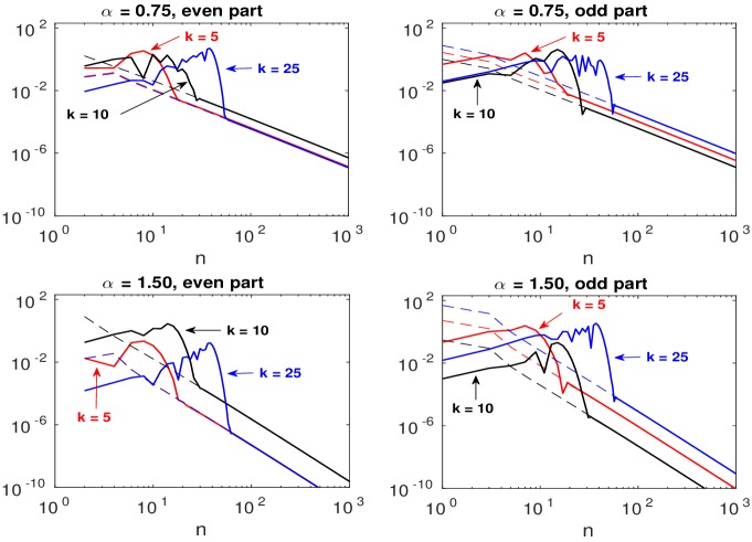
Figure 1: The coefficients $|c_{n}|$ (solid lines) and $|\hat{c}_{n}|$ (dashed lines) for $q(x)=\mathrm{e}^{x}.$

In Figure 1, some numerical illustrations of the estimates in (58) (left plots) and (59) (right plots) have been reported for $q(x)=\mathrm{e}^{x},$ $\alpha=0.75,1.5$ and $k=5,10,25.$ As one can see, for this example, such approximations of the coefficients are rather accurate for each $n\geq 3k.$

Before proceeding, we need the following notation. For each $\nu>0$ and $x\in(0,1)$ let

$$J(x,\nu,\mu)\equiv\int_{0}^{x}t^{\nu-1}(1-t)^{\mu-1}dt=\frac{x^{\nu}\,(1-x)^{\mu}}{\nu}{}_{2}F_{1}(1,\nu+\mu;1+\nu;x)$$ (60)

where the second equality is an application of Euler’s hypergeometric transformations [1]. By using a suitable Taylor expansion one deduces that

• if $x\rightarrow 0^{+}$ then

  $$J(x,\nu,\mu)=\frac{x^{\nu}\,(1-x)^{\mu}}{\nu}\left(1+O(x)\right);$$ (61)

• if $\mu<0$ then ${}_{2}F_{1}(1,\nu+\mu;1+\nu;1)=-\nu/\mu$ and consequently

  $$J(x,\nu,\mu)=-\frac{x^{\nu}\,(1-x)^{\mu}}{\mu}\left(1+o(1)\right),\quad{\mbox{a}s\,\,}x\nearrow 1^{-}.$$ (62)

  More precisely if $\mu<-1$ then $\left.\frac{d}{dx}{}_{2}F_{1}(1,\nu+\mu;1+\nu;x)\right|_{x=1}=\frac{(\nu+\mu)\nu}{(\mu+1)\mu}.$ This implies that

  $$J(x,\nu,\mu)=-\frac{x^{\nu}\,(1-x)^{\mu}}{\mu}\left(1+\frac{\nu+\mu}{\mu+1}(1-x)+o((1-x))\right).$$ (63)

We are now ready for the analysis of the entries of the local truncation error in (50).

Theorem 4.2

Let ${\alpha}\in(0,2)$ and suppose that $q$ verifies the assumptions H1 and H2. If $k$ is the index of the eigenvalue and $N_{0}$ is sufficiently larger than $k,$ then for each $N\geq N_{0}$ one has

$$|\tau_{m}^{(N)}|\leq\frac{C_{0}}{2\alpha N^{4\alpha+2}}\left(1-\frac{m^{2}}{N^{2}}\right)^{-\alpha},\qquad m=0,1,\ldots,N-1,$$ (64)

where $C_{0}$ is a constant independent of $N.$

Proof By using an integral estimate, from (50), (27), (43) and (57) one deduces that there exist a constant $C_{0},$ independent of $N$ and $m,$ such that

$$|\tau_{m}^{(N)}|\leq\sum_{n=N}^{\infty}|u_{mn}||c_{n}|\leq C_{0}\int_{N}^{\infty}(n^{2}-m^{2})^{-{\alpha}-1}n^{-2{\alpha}-1}dn\equiv C_{0}I_{m}^{(N)}.$$ (65)

If $m>0$ and if we apply the change of variable $n=mt^{-1/2}$ then, after some computation, from (60) with $\nu=2{\alpha}+1$ and $\mu=-{\alpha},$ we get

$$I_{m}^{(N)} = \frac{1}{2m^{4{\alpha}+2}}\,J\left(m^{2}/N^{2},2{\alpha}+1,-{\alpha}\right)$$

$$= \frac{1}{2(2{\alpha}+1)N^{4{\alpha}+2}}\,\left(1-\frac{m^{2}}{N^{2}}\right)^{-{\alpha}}\,{}_{2}F_{1}(1,{\alpha}+1;2{\alpha}+2;m^{2}/N^{2}).$$

It is not difficult to verify that this equality holds true also for $m=0.$ We observe that ${}_{2}F_{1}(1,{\alpha}+1;2{\alpha}+2;x)$ is increasing over $[0,1]$ and its value at $x=1$ is $(2{\alpha}+1)/{\alpha}.$ Therefore

$$I_{m}^{(N)}\leq\frac{1}{2{\alpha}N^{4{\alpha}+2}}\,\left(1-\frac{m^{2}}{N^{2}}\right)^{-{\alpha}}$$

which, together with (65), gives (64). $\Box$

The immediate consequence of this result is that the first and the last entries of $\mbox{\boldmath$\tau$}^{(N)}$ behave like $O(N^{-4{\alpha}-2})$ and $O(N^{-3{\alpha}-2}),$ respectively.
The following theorem completes the error analysis in the eigenvalue approximation.

Theorem 4.3

If the hypotheses of the previous theorem hold true then there exist a constant $C,$ independent of $N,$ such that

$$|\lambda-\lambda^{(N)}|\leq CN^{-(4{\alpha}+2)}.$$ (66)

Proof From (47)-(49), we deduce that there exist a constant $C_{1}$ such that

$$|\lambda-\lambda^{(N)}|=|{\mathbf{c}}_{N}^{T}\mbox{\boldmath$\tau$}^{(N)}+(\mbox{\boldmath$\xi$}_{N}-{\mathbf{c}}_{N})^{T}\mbox{\boldmath$\tau$}^{(N)}|/|(\mbox{\boldmath$\xi$}_{N}^{T}B_{N}{\mathbf{c}}_{N}|\leq C_{1}|{\mathbf{c}}_{N}^{T}\mbox{\boldmath$\tau$}^{(N)}|.$$

Now, by virtue of Theorem 4.1 we have that $|c_{m}|\sim m^{-2{\alpha}-1}$ for each $m\geq S=S(k),$ being $k$ the index of the eigenvalue. Therefore, from the previous theorem, we get

$$|{\mathbf{c}}_{N}^{T}\mbox{\boldmath$\tau$}^{(N)}| \leq \sum_{m=0}^{S-1}|c_{m}||\tau_{m}^{N}|+\sum_{m=S}^{N-1}|c_{m}||\tau_{m}^{N}|$$

$$\leq \frac{C_{2}}{N^{4{\alpha}+2}}\left(1+\int_{S}^{N-1}m^{-2{\alpha}-1}\left(1-\frac{m^{2}}{N^{2}}\right)^{-{\alpha}}dm\right),$$

where $C_{2}$ is a further suitable constant. If we apply the change of variable $t=1-m^{2}/N^{2}$ we obtain

$$\int_{S}^{N-1}m^{-2{\alpha}-1}\left(1-\frac{m^{2}}{N^{2}}\right)^{-{\alpha}}dm=\frac{1}{2N^{2{\alpha}}}\int_{x_{0}}^{x_{1}}t^{-{\alpha}}(1-t)^{-{\alpha}-1}dt\equiv\frac{\tilde{I}^{(N)}}{2N^{2{\alpha}}},$$

where

$$x_{0}=(2N-1)/N^{2}\approx 0,\qquad x_{1}=1-S^{2}/N^{2}\approx 1.$$ (67)

It follows that (66) holds true provided that $\tilde{I}^{(N)}=O(N^{2{\alpha}}).$ This fact can be verified, after some computation, for ${\alpha}=1.$ If ${\alpha}\in(0,1)$ then from (60), with $\nu=1-{\alpha}>0$ and $\mu=-{\alpha},$ (61)-(62) and (67) we get

$$\tilde{I}^{(N)}=J\left(x_{1},1-{\alpha},-{\alpha}\right)-J\left(x_{0},1-{\alpha},-{\alpha}\right)=O(N^{2{\alpha}}).$$

Finally, if ${\alpha}\in(1,2)$ then with an integration by parts and by using (60) with $\nu=2-{\alpha}>0$ and $\mu=-{\alpha}-1,$ see also (61)-(63) and (67), we obtain

$$\tilde{I}^{(N)} = \frac{1}{1-{\alpha}}\left.t^{1-{\alpha}}(1-t)^{-{\alpha}-1}\right|_{x_{0}}^{x_{1}}-\frac{{\alpha}+1}{1-{\alpha}}\int_{x_{0}}^{x_{1}}t^{1-{\alpha}}(1-t)^{-{\alpha}-2}dt$$

$$= \frac{1}{1-{\alpha}}\left.t^{1-{\alpha}}(1-t)^{-{\alpha}-1}\right|_{x_{0}}^{x_{1}}$$

$$- \frac{1+{\alpha}}{1-{\alpha}}\left(J(x_{1},2-{\alpha},-1-{\alpha})-J(x_{0},2-{\alpha},-1-{\alpha})\right)$$

$$= \frac{x_{0}^{1-{\alpha}}(1-x_{0})^{-{\alpha}-1}}{{\alpha}-1}\left(1+O(x_{0})\right)$$

$$+ \frac{x_{1}^{1-{\alpha}}(1-x_{1})^{-{\alpha}-1}}{1-{\alpha}}\left(1-x_{1}(1-(1-2{\alpha})(1-x_{1})/{\alpha}+o(1-x_{1}))\right)$$

$$= O(N^{{\alpha}-1})+\frac{x_{1}^{1-{\alpha}}(1-x_{1})^{-{\alpha}}}{1-{\alpha}}\left(1+(1-2{\alpha})x_{1}/{\alpha}+o(1))\right)$$

$$= O(N^{{\alpha}-1})+O(N^{2{\alpha}})=O(N^{2{\alpha}}),$$

which completes the proof. $\Box$

5 Conditioning analysis

We now discuss the conditioning of the numerical eigenvalues with respect to a perturbation of the potential. For a fixed $N,$ let $\lambda^{(N)}\equiv\lambda_{k}^{(N)}(q)$ and $\mbox{\boldmath$\xi$}_{N}\equiv\mbox{\boldmath$\xi$}_{k,N}(q)$ be the $k$-th numerical eigenvalue and the corresponding eigenvector as defined in (25). In addition, let $y^{(N)}(x)=y^{(N)}_{k}(x)$ be the resulting approximation of $y(x)=y_{k}(x)$ specified in (24). If we apply the matrix method to problem (1)-(2) with perturbed potential $\hat{q}(x)\approx q(x)$ then (25) becomes

$$\left(A_{N}+\hat{Q}_{N}\right)\hat{\mbox{\boldmath$\xi$}}_{k,N}(\hat{q})=\lambda_{k}^{(N)}(\hat{q})B_{N}\hat{\mbox{\boldmath$\xi$}}_{k,N}(\hat{q})$$

where the entries of $\hat{Q}_{N}$ are given by, see (26),

$$\hat{q}_{mn}=\langle P_{m}^{({\alpha/2})},\hat{q}P_{n}^{({\alpha/2})}\rangle_{{\alpha}},\quad m,n=0,\ldots N-1.$$

With these notations, we can prove the following result which concerns the case of a small perturbation of $q,$ i.e. of the initial datum.

Proposition 5.1

If $\|q-\hat{q}\|_{\infty}$ is small enough then

$$\left|\lambda_{k}^{(N)}(q)-\lambda_{k}^{(N)}(\hat{q})\right|\lesssim\|q-\hat{q}\|_{\infty},\quad k=0,1,\ldots,N-1.$$

Proof We observe that $(A_{N}+Q_{N},B_{N})$ is a symmetric (hermitian) definite pair, see [29] and Remark 3.2. Hence, by using standard arguments, it is not difficult to obtain that if $\|q-\hat{q}\|_{\infty}$ is sufficiently small then

$$\left|\lambda_{k}^{(N)}(q)-\lambda_{k}^{(N)}(\hat{q})\right| = \left|\frac{\mbox{\boldmath$\xi$}_{k,N}^{T}(q)\left(Q_{N}-\hat{Q}_{N}\right)\mbox{\boldmath$\xi$}_{k,N}(\hat{q})}{\mbox{\boldmath$\xi$}_{k,N}^{T}(q)B_{N}\mbox{\boldmath$\xi$}_{k,N}(\hat{q})}\right|$$

$$\approx \left|\frac{\mbox{\boldmath$\xi$}_{k,N}^{T}(q)\left(Q_{N}-\hat{Q}_{N}\right)\mbox{\boldmath$\xi$}_{k,N}(q)}{\mbox{\boldmath$\xi$}_{k,N}^{T}(q)B_{N}\mbox{\boldmath$\xi$}_{k,N}(q)}\right|$$

$$= \left|\frac{\displaystyle\int_{-1}^{1}(q(x)-\hat{q}(x))\left(y_{k}^{(N)}(x)\right)^{2}\,dx}{\displaystyle\int_{-1}^{1}\left(y_{k}^{(N)}(x)\right)^{2}\,dx}\right|\leq\|q-\hat{q}\|_{\infty}.$$

$\Box$

The numerical eigenvalues are therefore definitely well-conditioned with respect to a perturbation of the potential. This fact and Remark 3.3 suggest to consider a perturbed problem with $q$ replaced by $q_{L}\in\Pi_{L},$ the space of polynomials of maximum degree $L,$ where $L$ represents a further parameter to be specified by the user (in addition to $N,$ the order of the generalized matrix eigenvalue problem). In this way, in fact, the computation of $Q_{N}$ is simple and the resulting approximation of the eigenvalue verifies

$$\left|\lambda_{k}-\lambda_{k}^{(N)}(q_{L})\right|\leq\left|\lambda_{k}-\lambda_{k}^{(N)}(q)\right|+\left|\lambda_{k}^{(N)}(q)-\lambda_{k}^{(N)}(q_{L})\right|$$

which is approximately equal to $\left|\lambda_{k}-\lambda_{k}^{(N)}(q)\right|$ if $q_{L}$ is chosen properly.
In more details, even though different strategies are possible, we decided to select $q_{L}$ as the following partial sum of the Fourier-Legendre series of $q$

$$q_{L}(x)=\sum_{j=0}^{L}\tilde{q}_{j}P_{j}^{(0)}(x),\qquad\tilde{q}_{j}=\frac{\langle q,P_{j}^{(0)}\rangle_{0}}{\langle P_{j}^{(0)},P_{j}^{(0)}\rangle_{0}}=\frac{(2j+1)\,\langle q,P_{j}^{(0)}\rangle_{0}}{2},$$ (68)

which converges in uniform norm versus $q$ as $L$ increases if $q$ is analytic on the Bernstein ellipse. One motivation that lead us to consider this approach is that $q$ and $q_{L}$ have the same mean value (see (6) and the third example in Section 6). It must be said, in fact, that all our experiments suggest that the upper bound established in Proposition 5.1 may be not sharp if $\bar{q}=\bar{\hat{q}},$ $N$ is sufficiently large and $k/N<1/2.$ Finally, we observe that we can approximate $\langle q,P_{j}^{(0)}\rangle_{0}=\int_{-1}^{1}q(x)P_{j}^{(0)}(x)dx$ by applying a standard Gaussian quadrature formula or, for example, the algorithm described in [16].

6 Numerical experiments

The described method has been implemented in MATLAB (version R2015b) and the generalized matrix eigenvalue problem (25) has been solved by using the eig or the eigs (with option SM) commands depending on the number of eigenvalues we were interested in. For the approximation of the coefficients $\tilde{q}_{j}$ in (68) we have applied the standard Gaussian quadrature formula with degree of precision $\max(2L+1,11)$ (the function legpts included in Chebfun v4.3.2987 has been used for the computation of its nodes and weights). Concerning the choice of $L,$ we always select it in such a way that $\|q-q_{L}\|_{\infty}$ is of the order of the machine precision. For the estimate of the error in the approximation of $\lambda_{k}$ we consider as “exact” the corresponding numerical eigenvalue obtained with matrices of size $N_{\mathrm{true}}\gg N$ with $N_{\mathrm{true}}=N_{\mathrm{true}}(k,\alpha).$ In fact, it is important to underline the fact that if $\alpha\in(0,2)$ then the exact eigenvalues are not known in closed form even for $q$ identically zero in $(-1,1)$ and that, differently with respect to classical Sturm-Liouville problems, nowadays it is not yet available a well-established numerical software for the solution of the eigenvalue problem we have studied in this paper.

As first examples, we solved the problems with $q(x)=2x(x+1)$ and $q(x)=\mbox{e}^{\pi(x+1)/2}$ for several values of $\alpha$ and $N.$ Clearly, see (68), for the first potential we set $L=2$ while for the second one we choose $L=15.$ In Figures 2,3, the errors in the resulting approximation of the eigenvalues have been reported with, as we are going to do for all examples, a logarithmic scale on the abscissae. As one can see, in both cases, as soon as $N$ is sufficiently larger than the index of the eigenvalue $k,$ it results

$$\log_{10}(|\lambda_{k}-\lambda_{k}^{(N)}|)\sim-p\log_{10}(N).$$

Estimates of the various values of $p,$ determined with a least-square approximation, are listed in Table 1. It is evident that $p\approx(2+4\alpha)$ in agreement with Theorem 4.3.

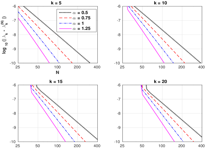
Figure 2: Errors in the approximation of the eigenvalues for $q(x)=2x(x+1).$

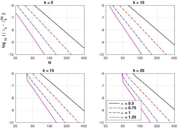
Figure 3: Errors in the approximation of the eigenvalues for $q(x)=\mbox{e}^{\pi(x+1)/2}.$

$q(x)=2x(x+1)$
$k$	$\alpha=0.50$	$\alpha=0.75$	$\alpha=1.00$	$\alpha=1.25$
5	3.99	4.94	5.86	6.79
10	3.99	4.96	5.94	6.92
15	3.99	4.94	5.89	6.84
20	4.00	4.96	5.94	6.92
$q(x)=\mbox{e}^{\pi(x+1)/2}$
$k$	$\alpha=0.50$	$\alpha=0.75$	$\alpha=1.00$	$\alpha=1.25$
5	4.00	4.96	5.91	6.85
10	4.00	4.95	5.91	6.88
15	4.01	4.95	5.90	6.85
20	4.01	4.95	5.92	6.91

Table 1: Estimates of the order of convergence in the eigenvalue approximations.

The aim of this second example is that of showing experimentally the growth of the error in the eigenvalue approximation with respect to the index $k$ for a fixed $N.$ In all our experiments it seems that if $q$ verifies the assumptions H1 and H2 and if $k/N$ is sufficiently small then

$$|\lambda_{k}-\lambda_{k}^{(N)}|=O\left(k^{r}N^{-2-4{\alpha}}\right),\qquad r=3{\alpha}.$$

This can be partially explained by observing that $\lambda_{k}$ grows like $k^{\alpha},$ see (5)-(6), and, consequently, see (50), (55)-(56) and (58)-(59), the first entries of the local truncation error behave like $k^{2{\alpha}}.$ Finally, by using (48)-(49) and (7), one deduces that the denominator in (47) decreases like $k^{-{\alpha}}$ (this fact is rather simple to be verified for ${\alpha}=2$ and $q\equiv 0$ over $(-1,1)$ since the exact eigenfunctions are known in closed form). All these arguments lead to the value of $r$ previously specified. As an example, in Figure 4 we report the errors in the eigenvalue approximations versus the index for $q(x)=(x+1)/(2(x^{2}+1))$ and for four values of ${\alpha}.$ In addition, we list estimates of the corresponding $r$’s determined with a least-square fitting.

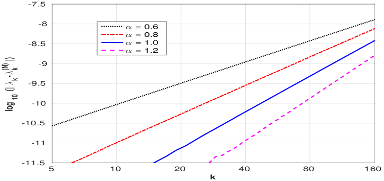
$\alpha$	$r$
0.6	1.82
0.8	2.41
1.0	3.01
1.2	3.60

Figure 4: Errors in the approximation of the eigenvalues versus their index for $q(x)=(x+1)/(2(x^{2}+1))$ with $N=320$ and $L=37.$

The third example is in support of the asymptotic estimate in (6). In particular, in Figure 5, we report $\log_{10}\left(|\lambda_{k}^{(N)}(q)-\lambda_{k}^{(N)}(0)-\bar{q}|\right)$ versus $k,$ for $q(x)=-\cos(3x)+\sin(2x)$, with $L=18$, $N=1000$, and $\alpha=0.7,1.1,1.5,1.9.$ As one can see, for each $\alpha,$ $\lambda_{k}^{(N)}$ approaches $\lambda_{k}^{(N)}(0)+\bar{q}$ as $k$ increases and this is in perfect agreement with (6) by considering also that $q$ and $q_{L}$ in (68) have the same mean value. As done in the previous examples, we apply a least-square fitting to determine the values of $\eta$ such that $|\lambda_{k}^{(N)}(q)-\lambda_{k}^{(N)}(0)-\bar{q}|=O(k^{-\eta})$ and the resulting exponents are listed in the table on the right of the same figure. For this example, we observe that $\eta\approx\alpha.$

Finally, we consider the infinite potential well, i.e. $q(x)=0$ for each $x\in(-1,1),$ with $\alpha=1.25$ and $\alpha=1.75.$ The variations in the numerical approximations of its first two eigenvalues (sometimes called the energies of the ground and of the first excited states) provided by the method proposed in this paper are of the order of the machine precision for each $N\geq 150.$ We then compare $\lambda_{0}^{(150)}$ and $\lambda_{1}^{(150)}$ with the numerical eigenvalues given by the methods proposed by

• Ortigueira/Zoia et al. in [25, 35];

• Tian et al. in [31];

• Duo and Zhang in [10].

We shall call $\mu_{k}^{(N)}$ the estimate of $\lambda_{k}$ provided by one of the previous three methods with a matrix of order $N.$ The results so obtained are reported in Figure 6. It is evident that $|\lambda_{k}^{(150)}-\mu_{k}^{(N)}|$ always decreases at the same rate; more precisely we have verified that such difference behaves like $O(N^{-1}).$ Finally, it is important to mention the fact that we have done similar experiments with other potentials and that the method that we propose turns out to be absolutely competitive with the other three ones in all our tests.

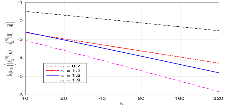
$\alpha$	$\eta$
0.7	0.70
1.1	1.09
1.5	1.48
1.9	1.86

Figure 5: Errors of the asymptotic estimate $\lambda_{k}^{(N)}(q)\approx\lambda_{k}^{(N)}(0)+\bar{q}$ for $q(x)=-\cos(3x)+\sin(2x)$ with $L=18$ and $N=1000.$

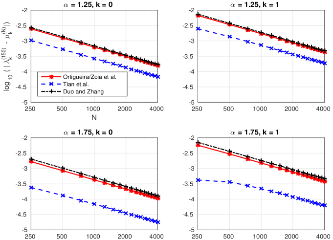
Figure 6: Comparison of the estimates of the first two eigenvalues of the infinite potential well problem provided by our method with $N=150$ and by the schemes proposed in [25, 35, 31, 10] with various values of $N.$

References

• [1] M. Abramowitz, I. A. Stegun, Handbook of Mathematical Functions, Dover, New York (1972).
• [2] G.E.  Andrews, R. Askey, R. Roy, Special Functions, Encyclopedia of Mathematics and its Applications, 71, Cambridge University Press, Cambridge (1999).
• [3] R. Bañuelos, T. Kulczycki, The Cauchy process and the Steklov problem, J. Funct. Anal. 211, no. 2, 355–423 (2004).
• [4] C. Beattie, An extension od Aronszajn’s rule: slicing the spectrum for intermediate problems, SIAM J. Numer. Anal. 24, no. 4, 828–843 (1987).
• [5] J. P. Borthagaray, L. M. Del Pezzo, S. Martínez, Finite element approximation for the fractional eigenvalue problem, March 2016, arXiv:1603.00317.
• [6] K. Bogdan, T. Byczkowski, T. Kulczycki, M. Ryznar, R. Song, Z.  Vondraček, Potential analysis of stable processes and its extensions, Lecture Notes in Mathematics 1980, Springer-Verlag, Berlin (2009).
• [7] C. Çelik, M. Duman, Crank-Nicolson method for the fractional diffusion equation with the Riesz fractional derivative, J. Comput. Phys. 231, no. 4, 1743-1750 (2012).
• [8] Z. Q. Chen, R. Song, Two-sided eigenvalue estimates for subordinate processes in domains, J. Funct. Anal. 226, no. 1, 90-113 (2005).
• [9] R. D. DeBlassie, Higher order PDEs and symmetric stable processes, Probab. Theory Related Fields 129, no. 4, 495-536 (2004).
• [10] S. Duo, Y. Zhang, Computing the Ground and First Excited States of the Fractional Schrödinger Equation in an Infinite Potential Well, Commun. Comput. Phys. 18, no. 2, 321-350 (2015).
• [11] B. Dyda, A. Kuznetsov, M. Kwaśnicki, Eigenvalues of the fractional Laplace operator in the unit ball, September 2015, arXiv:1509.08533.
• [12] B. Dyda, A. Kuznetsov, M. Kwaśnicki, Fractional Laplace operator and Meijer G-function, Constr. Approx. in press (2016).
• [13] A. Erdélyi, W. Magnus, F.  Oberhettinger, F. G. Tricomi, Tables of Integral Transforms, Vol. II. Based, in part, on notes left by Harry Bateman. McGraw-Hill Book Company, Inc., New York-Toronto-London (1954).
• [14] G. H. Golub, J. H. Welsch, Calculation of Gauss quadrature rules, Math. Comp. 23 (1969), 221-230.
• [15] A. Guerrero, M. A. Moreles, On the numerical solution of the eigenvalue problem in fractional quantum mechanics, Commun. Nonlinear Sci. Numer. Simul. 20, no. 2, 604-613 (2015).
• [16] A. Iserles, A fast and simple algorithm for the computation of Legendre coefficients, Numer. Math. 117, no. 3, 529-553 (2011).
• [17] M. Klimek, O. P. Agrawal, On a regular fractional Sturm–Liouville problem with derivatives of order in $(0,1),$ in: Proceedings of 13th International Carpathian Control Conference (ICCC) (2012).
• [18] M. Kwaśnicki, Spectral analysis of subordinate Brownian motions on the half-line, Studia Math., 206, 211-271 (2011).
• [19] M. Kwaśnicki, Eigenvalues of the fractional Laplace operator in the interval, J. Funct. Anal. 262, no. 5, 2379-2402 (2012).
• [20] M. Kwaśnicki, Ten equivalent definitions of the fractional laplace operator, September 2015, arXiv:1507.07356v2
• [21] N. Laskin, Fractional quantum mechanics and Lévy path integrals, Phys. Lett. A, 268, no. 4–6, 298-305 (2000).
• [22] N. Laskin, Fractals and quantum mechanica, Chaos, 10, no. 4, 780-790 (2000).
• [23] Y. Luchko, Fractional Schrödinger equation for a particle moving in a potential well, J. Math. Phys., 54, no. 1, 012111, 10 pp. (2013).
• [24] F. Mainardi, Yu. Luchko, G. Pagnini, The fundamental solution of the space-time fractional diffusion equation, Frac. Calc. Appl. Anal. 4, no. 2, 153-192 (2001).
• [25] M.D. Ortigueira, Riesz potential operator and inverses via fractional centred derivatives, Int. J. of Math. and Mathematical Sciences Article ID 48391, 1-12 (2006).
• [26] I. Podlubny, Fractional differential equations. An introduction to fractional derivatives, fractional differential equations, to methods of their solution and some of their applications, Mathematics in Science and Engineering, 198. Academic Press, Inc., San Diego, CA (1999).
• [27] J. Pöschel, E. Trubowitz, Inverse spectral theory, Pure and Applied Mathematics, 130, Academic Press, Inc., Boston, MA (1987).
• [28] S. G. Samko, A. A. Kilbas, O. I. Marichev, Fractional Integrals and Derivatives: Theory and Applications, Gordon and Breach Science Publishers, Yverdon (1993).
• [29] G. W. Stewart, J. G. Sun, Matrix perturbation theory, Computer Science and Scientific Computing. Academic Press, Inc., Boston, MA (1990).
• [30] G. Szegő, Orthogonal polynomials. Fourth edition. American Mathematical Society, Colloquium Publications, Vol. XXIII. American Mathematical Society, Providence, R.I. (1975).
• [31] W. Tian, H. Zhou, W. Deng, A class of second order difference approximations for solving space fractional diffusion equations, Math. Comp. 84, 1703-1727 (2015).
• [32] H. Wang, On the optimal estimates and comparison of Gegenbauer expansion coefficients, SIAM J. Numer. Anal., 54, no 3, 1557-1581 (2016).
• [33] M. Zayernouri, G. E. Karniadakis, Fractional Sturm-Liouville eigen-problems: theory and numerical approximation, J. Comput. Phys., 252, 495-517 (2013).
• [34] M. Zayernouri, M. Ainsworth, G. E. Karniadakis, Tempered fractional Sturm–Liouville eigenproblems, SIAM J. Sci. Comput., 37, no. 4, A1777-A1800 (2015).
• [35] A. Zoia, A. Rosso, M. Kardar, Fractional Laplacian in bounded domains. Phys. Rev. E (3) 76, no. 2, 021116, 11 pp (2007).