Computer assisted proof of Shil’nikov homoclinics: with application to the Lorenz-84 model

Computer assisted proof of Shil’nikov homoclinics: with application to the Lorenz-84 model

Abstract

We present a methodology for computer assisted proofs of Shil’nikov homoclinic intersections. It is based on geometric bounds on the invariant manifolds using rate conditions, and on propagating the bounds by an interval arithmetic integrator. Our method ensures uniqueness of the parameter for which the homoclinic takes place. We apply the method for the Lorenz-84 atmospheric circulation model, obtaining a sharp bound for the parameter, and also for where the homoclinic intersection of the stable/unstable manifolds takes place.

Key words. Shil’nikov homoclinic, invariant manifolds, non-transversal intersections, computer assisted proofs

AMS subject classifications. 34C37, 37D05, 37D10, 65G20.

1 Introduction

A class of three dimensional systems with a homoclinic orbit for a three dimensional saddle-focus equilibrium point was studied by Shil’nikov in a series of papers (see for example [21], [22], [23]). The homoclinic (usually called the Shil’nikov homoclinic orbit), can bifurcate in simple as well as in a chaotic way. The type of bifurcation depends on the saddle quantity, a constant derived from the eigenvalues of the linearised vector field at the fixed point. If the saddle quantity is negative, then a unique and stable limit cycle bifurcates from the homoclinic orbit. (This is called the simple Shil’nikov bifurcation.) If it is negative, then there occurs infinitely many periodic orbits of saddle type and one speaks of the chaotic Shil’nikov bifurcation (see also [15]). Shil’nikov homoclinics are important, since they lead to interesting dynamics. For instance, when combined with the study of the separatrix value, once can infer from them the existence of a Lorenz type attractor in the system [26].

Detecting Shil’nikov homoclinic intersections analytically is difficult, since in most systems of interest the ODE does not have a closed-form solution. In this paper we present a computer assisted approach for such proofs. The method is based on computer assisted estimates on the stable and unstable manifolds, and their propagation using rigorous, interval arithmetic integrator along the flow.

Our estimates for the invariant manifolds are based on the method of ‘rate conditions’ from [3, 4]. These are related to the rate conditions of Fenichel [6, 7, 8, 9]. The difference is that our our rate conditions are derived based on the estimates on the derivative at a (large) neighbourhood of a normally hyperbolic manifold (in this paper this manifold will be a family of hyperbolic fixed points), and not at the manifold as is done by Fenichel. Since our estimates are more global, we are able to establish existence and obtain explicit bounds on the invariant manifolds within the investigated neighbourhood.

The bounds on the manifolds are then propagated along the flow using interval and arithmetic integrator. For the proof of a homoclinic intersection, we use a standard shooting argument, which is based on the Bolzano’s intermediate value theorem. We also keep track of the dependence of the manifolds on the parameter, which leads to a uniqueness argument for the intersection.

To demonstrate that our method is applicable we implement it for the Lorenz-84 system [17]. We make a list of conditions that need to be verified in order to obtain the existence and uniqueness of the intersection, and then validate them. The bounds obtained by us are quite sharp. We establish the intersection parameter with $10^{-9}$ order of accuracy, and the region where the intersection takes place with $10^{-7}$ order of accuracy. The Lorenz-84 model serves only as an example. Our method is general, and can be applied to other systems.

The only other computer assisted proof of Shil’nikov homoclinics known to us is the work of Wilczak [28]. This method uses a topological shadowing mechanism, which stems from the method of ‘covering relations’ [10, 11] (refered to also in literature as ‘correctly aligned windows’), and Lyapunov function type arguments close to the fixed points. Our method is different. We rely on explicit estimates on the manifolds and their slopes, which are derived from rate conditions. Our method implies that the intersection parameter is unique within the given range. The uniqueness was not investigated in [28]. In [28] it is shown that in the investigated system there is an infinite number of Shil’nikov homoclinics, that are derived from symbolic dynamics. We focus on a simpler setting where the intersection is unique.

The paper is organised as follows. Section 2 contains preliminaries. In section 3 we introduce the Lorenz-84 model. Section 4 contains the proof for Shil’nikov type bifurcations. The proof is based on an assumption that within the investigated neighbourhood of the family of hyperbolic fixed points we have estimates on their invariant manifolds. We discuss how to obtain such estimates in section 5. This is based on the ‘rate conditions’ method from [4, 3], adapted to our setting. In section 6 we extend the method to obtain bounds on the dependence of the manifolds on the parameter of the system. Finally, in section 7, we apply our method for the Lorenz-84 system.

2 Preliminaries

2.1 Notations

Throughout the paper, all norms that appear are standard Euclidean norms. We use a notation $B_{k}(p,R)$ to denote a ball in $\mathbb{R}^{k}$ of radius $R$ centered at $p$. We use a short hand notation $B_{k}\left(R\right)$ for a ball or radius $R$ in $\mathbb{R}^{k}$ centered at zero. For a set $A\subset\mathbb{R}^{k}$, we use $\overline{A}$ to denote its closure and $\partial A$ for its boundary, $\mathrm{int}A$ for its interior and $A^{c}$ for the complement. For a point $p=\left(x,y\right)$ we use a notation $\pi_{x}p$ and $\pi_{y}p$ to denote projections onto $x$ and $y$ coordinates, respectively. We use the notation $(v|w)$ for the scalar product between two vectors $v$ and $w$.

2.2 Interval Newton method

Let $X$ be a subset of $\mathbb{R}^{n}$. We shall denote by $[X]$ an interval enclosure of the set $X$, that is, a set

$$[X]=\Pi_{i=1}^{n}[a_{i},b_{i}]\subset\mathbb{R}^{n},$$

such that

$$X\subset[X].$$

Let $f:\mathbb{R}^{n}\to\mathbb{R}^{n}$ be a $C^{1}$ function and $U\subset\mathbb{R}^{n}$. We shall denote by $[Df(U)]$ the interval enclosure of a Jacobian matrix on the set $U$. This means that $[Df(U)]$ is an interval matrix defined as

$$[Df(U)]=\left\{A\in\mathbb{R}^{n\times n}|A_{ij}\in\left[\inf_{x\in U}\frac{df_{i}}{dx_{j}}(x),\sup_{x\in U}\frac{df_{i}}{dx_{j}}(x)\right]\text{ for all }i,j=1,\ldots,n\text{ }\right\}.$$

Theorem 1

[1] (Interval Newton method) Let $f:\mathbb{R}^{n}\rightarrow\mathbb{R}^{n}$ be a $C^{1}$ function and $X=\Pi_{i=1}^{n}[a_{i},b_{i}]$ with $a_{i}<b_{i}$. If $[Df(X)]$ is invertible and there exists an $x_{0}$ in $X$ such that

$$N(x_{0},X):=x_{0}-\left[Df(X)\right]^{-1}f(x_{0})\subset X,$$

then there exists a unique point $x^{\ast}\in X$ such that $f(x^{\ast})=0.$

The Interval Newton Method can be applied to find the eigenvalues and eigenvectors of a matrix.

2.3 Interval arithmetic enclosure for eigenvalues and eigenvectors

Let $A$ be an $n\times n$ real matrix. In this section we outline how to solve

$$Ax=\lambda x.$$ (1)

We consider two cases. In the first, both $\lambda$ and $x$ will be real, and in the second

$$\lambda =\rho+i\omega,$$

$$x =x_{\mathrm{re}}+ix_{\mathrm{im}},$$

will be complex.

In the first case, we fix the first coordinate $x_{1}$ of $x=\left(x_{1},\tilde{x}\right)$ and treat $\tilde{x}\in\mathbb{R}^{n-1}$ as a variable. (We can also set some other coordinate to be fixed, if needed.) We define $f:\mathbb{R}^{n}\rightarrow\mathbb{R}^{n}$ as

$$f\left(\lambda,\tilde{x}\right)=Ax-\lambda x.$$

We see that solving $f\left(\lambda,\tilde{x}\right)=0$ is equivalent to (1). A solution of $f\left(\lambda,\tilde{x}\right)=0$ can be established using the interval Newton method (Theorem 1).

In the second case, we can consider $x_{\mathrm{re}}=\left(x_{\mathrm{re},1},\tilde{x}_{\mathrm{re}}\right)$ and $x_{\mathrm{im}}=\left(x_{\mathrm{im},1},\tilde{x}_{\mathrm{im}}\right),$ treating $\tilde{x}_{\mathrm{re}},\tilde{x}_{\mathrm{im}}\in\mathbb{R}^{n-1}$ as variables and $x_{\mathrm{re},1},x_{\mathrm{im},1}$ as fixed parameters. (We can also fix some other coordinate than the first, if needed.) We can consider $f:\mathbb{R}^{2n}\rightarrow\mathbb{R}^{2n}$ defined as

$$f\left(\rho,\tilde{x}_{\mathrm{re}},\omega,\tilde{x}_{\mathrm{im}}\right)=\left(\begin{array}[]{c}Ax_{\mathrm{re}}-\rho x_{\mathrm{re}}+\omega x_{\mathrm{im}}\\ Ax_{\mathrm{im}}-\rho x_{\mathrm{im}}-\omega x_{\mathrm{re}}\end{array}\right).$$

Clearly $f\left(\rho,\tilde{x}_{\mathrm{re}},\omega,\tilde{x}_{\mathrm{im}}\right)=0$ is equivalent to (1), and the solution can again be established using the interval Newton method.

2.4 Linear approximation of solutions of ODEs

In this section we present a technical lemma. Consider an ODE

$$p^{\prime}=f(p),$$

where $f:\mathbb{R}^{n}\rightarrow\mathbb{R}^{n}$ is $C^{1}$. Let $\Phi_{t}$ be the flow of the above system.

Lemma 2

Let $U\subset\mathbb{R}^{n}$ be a convex compact set. Then there exsist a constant $M>0$ such that for any $t>0$ and any $p,q\in\mathbb{R}^{n}$ satisfying

$$\{\Phi_{-s}(p),\Phi_{-s}(q):s\in[0,t]\}\subset U,$$

we have

$$\Phi_{-t}(p)-\Phi_{-t}(q)=p-q-tC(p-q)+g(t,p,q),$$

for some matrix $C\in\left[Df\left(U\right)\right]$ (which can depend on $p$, $q$ and $t$)and some $g$ satisfying

$$\left\|g(t,p,q)\right\|\leq Mt^{2}\left\|p-q\right\|.$$

Proof. The proof is given in the Appendix.   

Remark 3

In Lemma 2 we move backwards in time along the flow. We set this up in this way, because later on in our application we will use the lemma in the context of unstable manifolds, where moving back in time along the flow we will converge towards a fixed point.

2.5 Logarithmic norms

Let us begin with defining some matrix functionals that will be used by us in further proofs. Let $\left\|\cdot\right\|$ be a given norm in $\mathbb{R}^{n}$. Let $A\in\mathbb{R}^{n\times n}$ be a square matrix. By $m(A)$ we will denote the following matrix functional:

$$m(A)=\min_{z\in\mathbb{R}^{n},\|z\|=1}\|Az\|.$$

Definition 4

The logarithmic norm of $A$, denoted by $l(A)$ by [19, 5, 12, 16], is defined as

$$l(A)=\lim_{h\rightarrow 0^{+}}\frac{\|I+hA\|-\|I\|}{h}.$$ (2)

Moreover

$$m_{l}(A)=\lim_{h\rightarrow 0^{+}}\frac{m(I+hA)-\|I\|}{h}$$ (3)

will be called the logarithmic minimum of $A$.

Lemma 5

If $\left\|\cdot\right\|$ is the Euclidean norm, then the following equalities hold

$$l(A) =\max\{\lambda\in\text{spectrum of }(A+A^{\top})/2\},$$ (4)

$$m_{l}(A) =\min\{\lambda\in\text{spectrum of }(A+A^{\top})/2\}.$$ (5)

Remark 6

Equality (4) is a well known result (see for instance [12]). Equation (5) is proven in [3].

Corollary 7

From Lemma 5, we see that $m_{l}(-A)=-l\left(A\right).$

Lemma 8

[3] Consider the Euclidean norm $\left\|\cdot\right\|$. Let $W\subset\mathbb{R}^{n\times n}$ be a compact set and let $t_{0}>0$. Then for any $t\in(0,t_{0}]$ and $A\in W$ the following equality holds

$$\|I+tA\|=1+tl(A)+r(t,A),$$

where

$$\|r(t,A)\|\leq Ct^{2},$$

for some constant $C=C(t_{0},W)$.

Lemma 9

[3] Consider the Euclidean norm $\left\|\cdot\right\|$. Let $W\subset\mathbb{R}^{n\times n}$ be a compact set and let $t_{0}>0$. Then for any $t\in(0,t_{0}]$ and $A\in W$ the following equality holds

$$m(I+tA)=1+tm_{l}(A)+r(t,A)$$

where

$$\|r(t,A)\|\leq Ct^{2}$$

for some constant $C=C(t_{0},W)$.

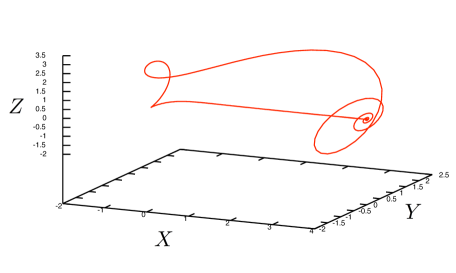
Figure 1: The Shil’nikov homoclinic in the Lorenz-84 model for $F=4.0$ and $G\simeq 0.08$.

3 Lorenz-84 Atmospheric Circulation Model

The Lorenz-84 Model was introduced by Lorenz in [17]. It is a low-order model for the long-term atmospheric circulation. It is considered as the simplest model capable of representing the basic features of the so-called Hadley circulation. Therefore, it has been widely used in meteorogical studies. The detailed analysis of this model can be found in [27]. The model equations are

$$\left\{\begin{array}[]{rl}\dot{X}&=-Y^{2}-Z^{2}-aX+aF,\\ \dot{Y}&=XY-bXZ-Y+G,\\ \dot{Z}&=bXY+XZ-Z,\end{array}\right.$$ (6)

where variable $X$ represents the strength of the globally averaged westerly wind current and variables $Y$ and $Z$ are the strength of the cosine and sine phases of a chain of superposed waves transporting heat poleward. $F$ and $G$ represent the thermal forcing terms, and the parameter $b$ stands for the advection strength of the waves by the westerly wind current. The coefficient $a$, if less than 1, allows the westerly wind current to damp less rapidly than the waves. The time unit is equal to the damping time of the waves and it is estimated to be five days.

In their paper [25], A.Shil’nikov, G.Nicolis and C.Nicolis carry out a detailed bifurcation analysis for the Lorenz-84 Model with parameters $a$ and $b$ set to classical values $\frac{1}{4}$ and $4$ respectively (these values were also considered in many other works, see for example [2], [17], [18]). The authors identify the types of the equilibrium points depending on the choice of the domain for the parameters $F$ and $G$. They show that the problem has either one, two or three equilibrium points. If parameters $F$ and $G$ are chosen from a proper domain, one of the fixed points, denoted in [25] as $O_{1}$, is saddle-focus. The paper [25] presents a numerical calculations suggesting the existence of the homoclinic orbit passing through $O_{1}$ that is possesed by the system for $F\simeq 4.0$ and $G\simeq 0.08$. The homoclinic is depicted in Figure 1.

Following Shil’nikov et al. [25] we set parameters $a=\frac{1}{4}$ and $b=4$. In further sections we will use our method to rigourously enclose the stable and unstable manifolds, and to validate the existence of a homoclinic orbit for saddle-focus fixed point $O_{1}$. We prove that such an orbit exists for $F=4$, and some $G$, where

$$G\in\left[0.0752761095,0.07527611625\right].$$ (7)

Moreover, we show the uniqueness of such $G$ in the interval (7).

4 Establishing Shil’nikov homoclinics

Let us consider the three dimensional system given by the following ODE

$$p^{\prime}=f(p,\theta),$$ (8)

where $f:\mathbb{R}^{3}\times\mathbb{R}\rightarrow\mathbb{R}^{3}$ is $C^{1}$, and $\theta\in\Theta$ is a parameter, with $\Theta=[\theta_{l},\theta_{r}]\subset\mathbb{R}$. Let $\Phi_{t}(p,\theta)$ be the flow induced by (8).

Suppose that for $\theta\in\Theta$, system 8 has a smooth family of hyperbolic fixed points $p_{\theta}^{\ast}$, with two dimensional stable and one dimensional unstable eigenspace.

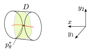
Figure 2: The local unstable manifold $W_{\theta}^{u}$ in red, and the local stable manifold $W_{\theta}^{s}$ in green.

Below we present a theorem, which allow us to prove the existence of a homoclinic orbit in the system. First we need to introduce some notation.

Let $\overline{B}_{u}\left(R\right)=\left[-R,R\right]\subset\mathbb{R}$, $\overline{B}_{s}\left(R\right)\subset\mathbb{R}^{2}$ and let

$$D=\overline{B}_{u}\left(R\right)\times\overline{B}_{s}\left(R\right)\subset\mathbb{R}^{3},$$

be a neighborhood of the smooth family of fixed points, meaning that we assume $p_{\theta}^{\ast}\in\mathrm{int}D$ for any $\theta\in\Theta$. The set $D$ will be fixed throughout the discussion. We denote by $W_{\theta}^{u}$ the local unstable manifold of $p_{\theta}^{\ast}$ in $D$ and by $W_{\theta}^{s}$ the local stable manifold of $p_{\theta}^{\ast}$ in $D$, i.e.

$$W_{\theta}^{u} =\left\{p\in D:\Phi_{t}\left(p,\theta\right)\in D\text{ for }t\leq 0\text{ and }\lim_{t\rightarrow-\infty}\Phi_{t}\left(p,\theta\right)=p_{\theta}^{\ast}\right\},$$ (9)

$$W_{\theta}^{s} =\left\{p\in D:\Phi_{t}\left(p,\theta\right)\in D\text{ for }t\geq 0\text{ and }\lim_{t\rightarrow+\infty}\Phi_{t}\left(p,\theta\right)=p_{\theta}^{\ast}\right\}.$$ (10)

We assume that $W_{\theta}^{u}$ and $W_{\theta}^{s}$ are graphs of $C^{1}$ functions

$$w^{u} :\overline{B}_{u}\left(R\right)\times\Theta\rightarrow\overline{B}_{s}\left(R\right),$$

$$w^{s} :\overline{B}_{s}\left(R\right)\times\Theta\rightarrow\overline{B}_{u}\left(R\right),$$

meaning that (see Figure 2)

$$W_{\theta}^{u} =\left\{\left(x,w^{u}\left(x,\theta\right)\right):x\in\overline{B}_{u}\left(R\right)\right\},$$

$$W_{\theta}^{s} =\left\{\left(w^{s}\left(y,\theta\right),y\right):y\in\overline{B}_{s}\left(R\right)\right\}.$$ (11)

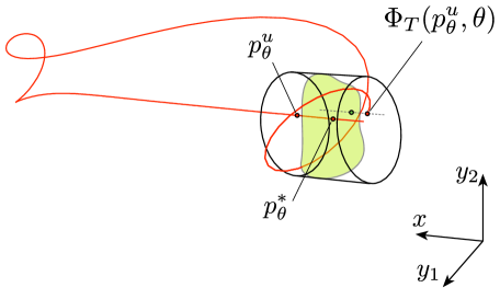
Figure 3: We have the $1$-dimensional unstable manifold of $p_{\theta}^{\ast}$ in red, and the $2$-dimensional local stable manifold $W_{\theta}^{s}$ in $D$ in green. The $h\left(\theta\right)$ is the signed distance along the $x$ coordinate between $W_{\theta}^{s}$ and $\Phi_{T}\left(p_{\theta}^{u},\theta\right)$; this is the distance along the dotted line on the plot.

Let

$$p_{\theta}^{u}:=\left(R,w^{u}\left(R,\theta\right)\right)\in\mathbb{R}^{3}.$$ (12)

Consider $T>0$ and assume that for all $\theta\in\Theta$, $\Phi_{T}\left(p_{\theta}^{u},\theta\right)\in D$. Let us define

$$h:\Theta\rightarrow\mathbb{R},$$

as

$$h\left(\theta\right)=\pi_{x}\Phi_{T}\left(p_{\theta}^{u},\theta\right)-w_{\theta}^{s}(\pi_{y}\Phi_{T}\left(p_{\theta}^{u},\theta\right)).$$ (13)

We now state a natural result, that $h\left(\theta\right)=0$ implies an intersection of the stable and unstable manifolds of $p_{\theta}^{\ast}$. (See Figure 3.)

Theorem 10

If

$$h(\theta_{l})<0\qquad\text{and}\qquad h(\theta_{r})>0$$ (14)

then there exists a $\psi\in\Theta$ for which we have a homoclinic orbit to $p_{\psi}^{\ast}$.

Moreover, if for all $\theta\in\Theta$, $h^{\prime}(\theta)>0$, then $\psi$ is the only parameter for which we have a homoclinic orbit satisfying $\Phi_{t}\left(p_{\theta}^{u},\theta\right)\in D$ for all $t>T$.

Proof. Since $w^{u}$, $w^{s}$ are $C^{1}$, also is $h$. From (14), by the Bolzano intermediate value theorem, it follows that there exists a $\psi\in\Theta$ for which $h\left(\psi\right)=0$. Let $q=\Phi_{T}(p_{\psi}^{u},\psi)$. Since $h\left(\psi\right)=0,$

$$q=\left(\pi_{x}q,\pi_{y}q\right)=\left(w_{\psi}^{s}(\pi_{y}q),\pi_{y}q\right).$$ (15)

Since $p_{\psi}^{u}\in W^{u},$ clearly $q=\Phi_{T}(p_{\psi}^{u},\psi)$ belongs to the unstable manifold of $p_{\psi}^{\ast}$. All points of the form $(w_{\psi}^{s}(y),y)$ belong to the stable manifold of $p_{\psi}^{\ast}$, hence by (15) so does $q$, and the stable and unstable manifolds intersect at $q$.

If $h^{\prime}\left(\theta\right)>0$ for all $\theta\in\Theta$, then $\psi$ is the only parameter for which $h$ is zero, hence for all $\theta\neq\psi$,

$$\pi_{x}\Phi_{T}\left(p_{\theta}^{u},\theta\right)\neq w_{\theta}^{s}(\pi_{y}\Phi_{T}\left(p_{\theta}^{u},\theta\right)).$$

This by (11), implies that for $\theta\neq\psi$, $\Phi_{T}\left(p_{\theta}^{u},\theta\right)\notin W_{\theta}^{s}$. By (10) this means that for some $t>T$, $\Phi_{t}\left(p_{\theta}^{u},\theta\right)\notin D$, or that we do not have a homoclinic for this parameter.   

Remark 11

The inequalities in (14) and the sign of $h^{\prime}$ in Theorem 10 can be reversed. Then the proof follows from mirror arguments.

To apply Theorem 10, we need to be able to compute estimates on $h$ and its derivative. We note that obtaining a rigorous bound on a time shift map $\Phi_{T}$ along the flow, and on its derivative, can be computed in interval arithmetic using the CAPD package. To compute $h$ and its derivative it is therefore enough to be able to obtain estimates on $w^{u},$ $w^{s}$ and their derivatives. We discuss how this can be achieved in interval arithmetic in subsequent sections 5 and 6. We use these, together with Theorem 10, to provide a computer assisted proof of a homoclinic intersection in the Lorenz-84 model, in section 7.

5 Bounds on unstable manifolds of hyperbolic fixed points

Consider an ODE

$$q^{\prime}=f\left(q\right),$$ (16)

and let

$$D=\overline{B}_{u}\left(R\right)\times\overline{B}_{s}\left(R\right)\subset\mathbb{R}^{u}\times\mathbb{R}^{s}$$

The results of this section are more general than the previously considered ode in $\mathbb{R}^{3}$, and here $u,s$ can be any natural numbers. We use a notation $x\in\mathbb{R}^{u}$ to stand for the unstable coordinate and $y\in\mathbb{R}^{s}$ for the stable coordinate. For us it will be enough if these coordinates are ‘roughly’ aligned with the eigenspaces of a fixed point. (We do not need to work with precisely linearised local coordinates.) We write $f(x,y)=(f_{x}(x,y),f_{y}(x,y))$, where $f_{x}$ is the projection onto $\mathbb{R}^{u}$ and $f_{y}$ is the projection onto $\mathbb{R}^{s}$.

Let $L>0$ be a fixed number. We define

$$\mu_{1} =\sup_{z\in D}\left\{l\left(\frac{\partial f_{y}}{\partial y}(z)\right)+\frac{1}{L}\left\|\frac{\partial f_{y}}{\partial x}(z)\right\|\right\},$$

$$\mu_{2} =\sup_{z\in D}\left\{l\left(\frac{\partial f_{y}}{\partial y}(z)\right)+\frac{1}{L}\left\|\frac{\partial f_{x}}{\partial y}(z)\right\|\right\},$$

$$\xi =m_{l}\left(\frac{\partial f_{x}}{\partial x}(D)\right)-\frac{1}{L}\sup_{z\in D}\left\|\frac{\partial f_{x}}{\partial y}(z)\right\|.$$

Definition 12

We say that the vector field $f$ satisfies rate conditions in $D$ if

$$\mu_{1}<0<\xi,$$ (17)

$$\mu_{2}<\xi.$$ (18)

Definition 13

We say that $D=\overline{B}_{u}\left(R\right)\times\overline{B}_{s}\left(R\right)$ is an isolating block for (16) if

1. For any $q\in\partial\overline{B}_{u}\left(R\right)\times\overline{B}_{s}\left(R\right)$,

   $$\left(\pi_{x}f(q)|\pi_{x}q\right)>0.$$

2. For any $q\in\overline{B}_{u}\left(R\right)\times\partial\overline{B}_{s}\left(R\right)$,

   $$\left(\pi_{y}f(q)|\pi_{y}q\right)<0.$$

Definition 14

We define the unstable set in $D$ as

$$W^{u}=\{z:\text{ }\Phi_{t}(z)\in D\text{ for all }t<0\}.$$

Theorem 15

Assume that $f$ is $C^{1}$ and satisfies rate conditions. Assume also that $D=\overline{B}_{u}\left(R\right)\times\overline{B}_{s}\left(R\right)$ is an isolating block for $f$. Then the set $W^{u}$ is a manifold, which is a graph over $\overline{B}_{u}\left(R\right)$. To be more precise, there exists a function

$$w^{u}:\overline{B}_{u}(R)\rightarrow\overline{B}_{s}(R),$$

such that

$$W^{u}=\left\{\left(x,w^{u}(x)\right):x\in\overline{B}_{u}(R)\right\}.$$

Moreover, $w^{u}$ is Lipschitz with constant $L$ and for $C=2R\left(1+1/L\right)$, for any $p_{1},p_{2}\in W^{u},$

$$\left\|\Phi_{-t}\left(p_{1}\right)-\Phi_{-t}\left(p_{2}\right)\right\|\leq Ce^{-t\xi}\qquad\text{for all }t>0.$$ (19)

Proof. The result follows directly from Theorem 30 from [3]. Theorem 30 in [3] is written in the context where apart from $x,y$ we have an additional ‘center’ coordinate, which is not present here. This is why the number of constants and rate conditions (17–18) for Theorem 15 is smaller than the number of constants and associated inequalities needed in [3]. The (17–18) imply all the needed assumptions of Theorem 30 from [3] in the absence of the center coordinate.   

In above theorem we ignore (fix) the parameter. The result can be extended to include the parameter as follows.

Theorem 16

Consider a parameter dependent ODE

$$p^{\prime}=f(p,\theta),$$

for $\theta\in\Theta$. Assume that the system has a smooth family of hypebolic fixed points $p_{\theta}^{\ast}$. Assume that for each (fixed) $\theta$, the vector field satisfies assumptions of Theorem 15. Then the family of unstable manifolds $W_{\theta}^{u}$ (as defined in (9)) of $p_{\theta}^{\ast}$ is given by a graph of a function

$$w^{u}:\overline{B}_{u}\left(R\right)\times\Theta\rightarrow\overline{B}_{s}\left(R\right),$$

(meaning that $W_{\theta}^{u}=\left\{\left(x,w^{u}(x,\theta)\right):x\in\overline{B}_{u}\left(R\right)\right\}$,) which is as smooth as $f$.

Proof. The existence of $w^{u}$ follows from Theorem 15. We need to justify its smoothness.

From the classical theory (see for instance [13],[14],[20]), we know that in a small neighbourhood $U$ of $\{(p_{\theta}^{\ast},\theta)|\theta\in\Theta\}$ (considered in the state space, extended to include the parameter), the family of local unstable manifolds exists, and is as smooth as $f$. Condition (19) ensures that the local manifold is propagated along the flow in the extended space to span the set $D\times\Theta$. Since $\Phi_{t}$ is as smooth as $f$, this establishes the smoothness of $w^{u}$.   

Remark 17

In this section we have focused on the unstable manifold. This method can also be applied to obtain bounds on a stable manifold. To do so one can simply change the sign of the vector field.

6 Dependence of the unstable manifold on parameters

In this section we consider the ODE of the form

$$p^{\prime}=f(p,\theta)$$ (20)

depending on the parameter $\theta\in\Theta$, where $p\in\mathbb{R}^{u}\times\mathbb{R}^{s}$ and $f:\mathbb{R}^{u}\times\mathbb{R}^{s}\times\Theta\rightarrow\mathbb{R}^{u}\times\mathbb{R}^{s}$ is $C^{1}$ function, with

$$f(x,y,\theta)=(f_{x}(x,y,\theta),f_{y}(x,y,\theta)).$$

Our aim know is to examine the nature of the dependency of function $w^{u}$, which parametrizes the unstable manifold in the stament of Theorem 15, on parameter $\theta$.

Let our coordinates be $(x,y,\theta)\in\mathbb{R}^{u}\times\mathbb{R}^{s}\times\mathbb{R}$, and let us consider the following sets:

$$J_{s}\left(q,M\right) =\left\{\left(x,y,\theta\right):\left\|\pi_{x,\theta}q-\left(x,\theta\right)\right\|\leq M\left\|\pi_{y}q-y\right\|\right\},$$

$$J_{cu}\left(q,M\right) =\left\{\left(x,y,\theta\right):\left\|\pi_{y}q-y\right\|\leq M\left\|\pi_{x,\theta}q-\left(x,\theta\right)\right\|\right\},$$

where $q\in\mathbb{R}^{u}\times\mathbb{R}^{s}\times\mathbb{R}$ and $M>0$. These sets represent cones depicted in Figure 4. Note that we have

$$\left(J_{cu}\left(q,1/M\right)\right)^{c}=\mathrm{int}J_{s}\left(q,M\right).$$ (21)

Figure 4: The cones $J_{s}(q,M_{1})$ and $J_{s}(q,M_{2})$ for $M_{1}=1$ and $M_{2}=\frac{1}{2}$.

Let us consider an ODE given by (20) in the state space extended by parameter, that is

$$\left(x^{\prime},y^{\prime},\theta^{\prime}\right)=\left(f_{x}\left(x,y,\theta\right),f_{y}\left(x,y,\theta\right),f_{\theta}(x,y,\theta)\right),$$ (22)

where $f_{\theta}(x,y,\theta)=0$. Let $\Phi_{t}(x,y,\theta)$ be the flow induced by (22).

Let $D=\overline{B}_{u}\left(R\right)\times\overline{B}_{s}\left(R\right)\subset\mathbb{R}^{u}\times\mathbb{R}^{s}$ and let us define

$$\mathcal{D}=D\times\Theta,$$

and the following constants:

$$\mu\left(M\right) =l\left(\frac{\partial f_{y}}{\partial y}\left(\mathcal{D}\right)\right)+M\left\|\frac{\partial f_{y}}{\partial\left(x,\theta\right)}\left(\mathcal{D}\right)\right\|,$$ (23)

$$\xi\left(M\right) =m_{l}\left(\frac{\partial f_{x,\theta}}{\partial\left(x,\theta\right)}\left(\mathcal{D}\right)\right)-\frac{1}{M}\left\|\frac{\partial f_{x,\theta}}{\partial y}\left(\mathcal{D}\right)\right\|.$$ (24)

Our objective will be to prove the following theorem:

Theorem 18

Consider that assumptions of Theorem 16 hold and that $M>0$ is such that

$$\mu\left(M\right)<0\qquad\text{and\qquad}\xi\left(M\right)>\mu\left(M\right).$$

Then

$$\left\|\frac{\partial w^{u}}{\partial\theta}\right\|\leq 1/M.$$

The proof of the theorem will be given at the end of the section. To show the result we shall need two technical lemmas.

Lemma 19

Assume that $M>0$ is such that

$$\mu\left(M\right)<0\qquad\text{and\qquad}\xi\left(M\right)>\mu\left(M\right).$$

Then there exists a $c>0$ and $t_{M}>0$ such that for any $q\in\mathcal{D}$ and $p\in J_{s}\left(q,M\right)\cap\mathcal{D},$ $p\neq q$, as long as $\{\Phi_{-t}(p),\Phi_{-t}(q):t\in[0,t_{M}]\}\subset\mathcal{D}$, the following inequality holds

$$\left\|\pi_{y}\left(\Phi_{-t}\left(p\right)-\Phi_{-t}\left(q\right)\right)\right\|>\left(1+ct\right)\left\|\pi_{y}\left(p-q\right)\right\|,$$ (25)

for any $t\in(0,t_{M})$. Moreover

$$\Phi_{-t}\left(p\right)\in J_{s}\left(\Phi_{-t}\left(q\right),M\right).$$ (26)

Proof. Take any $q\in\mathcal{D}$ and $p\in J_{s}\left(q,M\right)\cap\mathcal{D},$ $p\neq q$, and let $t>0$ be such that $\{\Phi_{-s}(p),\Phi_{-s}(q):s\in[0,t]\}\subset\mathcal{D}$.

Since $p\in J_{s}\left(q,M\right),$

$$\left\|\pi_{x,\theta}\left(p-q\right)\right\|\leq M\left\|\pi_{y}\left(p-q\right)\right\|.$$ (27)

As a consequence

$$\left\|p-q\right\|\leq\sqrt{M^{2}+1}\left\|\pi_{y}(p-q)\right\|.$$ (28)

Therefore since $p\neq q$ we must have

$$\left\|\pi_{y}(p-q)\right\|\neq 0.$$

On the other hand, from Lemma 2 it follows that for some $A\in\left[\frac{\partial f_{y}}{\partial y}\left(\mathcal{D}\right)\right]$ and $B\in\left[\frac{\partial f_{y}}{\partial\left(x,\theta\right)}\left(\mathcal{D}\right)\right]$

$$\pi_{y}\left(\Phi_{-t}\left(p\right)-\Phi_{-t}\left(q\right)\right) =\pi_{y}\left(p-q\right)-tA\pi_{y}\left(p-q\right)-tB\pi_{x,\theta}\left(p-q\right)$$

$$\quad+\pi_{y}g(t,p,q),$$

where $g$ satisfies $\left\|g(t,p,q)\right\|\leq\gamma_{1}t^{2}\left\|p-q\right\|$ for some constant $\gamma_{1}>0$. Observe that from (28) we have $\left\|g(t,p,q)\right\|\leq\gamma_{1}t^{2}\left\|\pi_{y}(p-q)\right\|$. From the above, and by using (27) in the second line, Lemma 9 in the third line, Corollary 7 in the fourth line, and (23) in the last line, we obtain

$$\left\|\pi_{y}\left(\Phi_{-t}\left(p\right)-\Phi_{-t}\left(q\right)\right)\right\| \geq\left\|\left(Id-tA\right)\pi_{y}\left(p-q\right)\right\|-t\left\|B\right\|\left\|\pi_{x,\theta}\left(p-q\right)\right\|$$

$$\quad-\gamma_{1}t^{2}\left\|\pi_{y}(p-q)\right\|$$

$$\geq\left(m\left(Id-tA\right)-tM\left\|B\right\|\right)\left\|\pi_{y}\left(p-q\right)\right\|$$

$$\quad-\gamma_{1}t^{2}\left\|\pi_{y}(p-q)\right\|$$

$$\geq\left(1+tm_{l}\left(-A\right)-tM\left\|B\right\|\right)\left\|\pi_{y}\left(p-q\right)\right\|$$

$$\quad-\gamma_{2}t^{2}\left\|\pi_{y}(p-q)\right\|$$

$$=\left(1+t\left(-l\left(A\right)-M\left\|B\right\|\right)\right)\left\|\pi_{y}\left(p-q\right)\right\|$$

$$\quad-\gamma_{2}t^{2}\left\|\pi_{y}(p-q)\right\|$$

$$\geq\left(1-t\mu\left(M\right)-\gamma_{2}t^{2}\right)\left\|\pi_{y}\left(p-q\right)\right\|,$$ (29)

where, in the light of Lemma 9, the third inequality is satisfied for any $t\in[0,t_{0}]$, where $t_{0}>0$. Taking a fixed $c\in\left(0,-\mu\left(M\right)\right)$, we see that there exists $t_{M}>0$ (independent of $p$ and $q$) such that for any $t\in(0,t_{M})$

$$\left\|\pi_{y}\left(\Phi_{-t}\left(p\right)-\Phi_{-t}\left(q\right)\right)\right\|>\left(1+tc\right)\left\|\pi_{y}\left(p-q\right)\right\|,$$

which proves (25).

Again from Lemma 2, we know that for some $A\in\left[\frac{\partial f_{x,\theta}}{\partial\left(x,\theta\right)}\left(\mathcal{D}\right)\right]$ and $B\in\left[\frac{\partial f_{x,\theta}}{\partial y}\left(\mathcal{D}\right)\right]$

$$\pi_{x,\theta}\left(\Phi_{-t}\left(p\right)-\Phi_{-t}\left(q\right)\right) =\pi_{x,\theta}\left(p-q\right)-tA\pi_{x,\theta}\left(p-q\right)-tB\pi_{y}\left(p-q\right)$$

$$\quad+\pi_{x,\theta}g(t,p,q).$$

Hence, using (27) in the second line, Lemma 8 in the third line, Corollary 7 in the fourth line and (24) in the last line,

$$\left\|\pi_{x,\theta}\left(\Phi_{-t}\left(p\right)-\Phi_{-t}\left(q\right)\right)\right\| \leq\left\|Id-tA\right\|\left\|\pi_{x,\theta}\left(p-q\right)\right\|+t\left\|B\right\|\left\|\pi_{y}\left(p-q\right)\right\|$$

$$\quad+\gamma_{1}t^{2}\left\|\pi_{y}(p-q)\right\|$$

$$\leq\left(\left\|Id-tA\right\|M+t\left\|B\right\|\right)\left\|\pi_{y}\left(p-q\right)\right\|$$

$$\quad+\gamma_{1}t^{2}\left\|\pi_{y}(p-q)\right\|$$

$$=M\left(\left(1+tl\left(-A\right)\right)M+\frac{1}{M}t\left\|B\right\|\right)\left\|\pi_{y}\left(p-q\right)\right\|$$

$$\quad+\gamma_{2}t^{2}\left\|\pi_{y}(p-q)\right\|$$

$$=M\left(\left(1-tm_{l}\left(A\right)\right)+\frac{1}{M}t\left\|B\right\|\right)\left\|\pi_{y}\left(p-q\right)\right\|$$

$$\quad+\gamma_{2}t^{2}\left\|\pi_{y}(p-q)\right\|$$

$$\leq\left(M-tM\xi\left(M\right)+\gamma_{2}t^{2}\right)\left\|\pi_{y}\left(p-q\right)\right\|,$$ (30)

where, in the light of Lemma 8, the third inequality is satisfied for any $t\in[0,t_{0}]$, where $t_{0}>0$. Since $\xi\left(M\right)>\mu\left(M\right),$ by combining (29) with (30), we see that for sufficiently small $t$,

$$\frac{\left\|\pi_{x,\theta}\left(\Phi_{-t}\left(p\right)-\Phi_{-t}\left(q\right)\right)\right\|}{\left\|\pi_{y}\left(\Phi_{-t}\left(p\right)-\Phi_{-t}\left(q\right)\right)\right\|}\leq\frac{\left(M-tM\xi\left(M\right)+\gamma_{2}t^{2}\right)\left\|\pi_{y}\left(p-q\right)\right\|}{\left(1-t\mu\left(M\right)-\gamma_{2}t^{2}\right)\left\|\pi_{y}\left(p-q\right)\right\|}\leq M.$$

This means that

$$\left\|\pi_{\theta,x}\left(\Phi_{-t}\left(p\right)-\Phi_{-t}\left(q\right)\right)\right\|\leq M\left\|\pi_{y}\left(\Phi_{-t}\left(p\right)-\Phi_{-t}\left(q\right)\right)\right\|,$$

which proves (26).   

We now return to studying (20). Let us assume that the system has a smooth family of hyperbolic fixed points $p_{\theta}^{\ast}\in\mathrm{int}D$, where $D=\overline{B}_{u}\left(R\right)\times\overline{B}_{s}\left(R\right)$. Let us also assume that for any given $\theta\in\Theta$ assumptions of Theorem 15 are satisfied. Let $w^{u}$ be the parameterisation from Theorem 16.

Lemma 20

If assumptions of Theorem 16 are satisfied and

$$\mu\left(M\right)<0,\qquad\text{\qquad}\xi\left(M\right)>\mu\left(M\right),$$

then for any $x_{1},x_{2}\in\overline{B}_{u}\left(R\right)$ and $\theta_{1},\theta_{2}\in\Theta$,

$$\left(x_{1},w^{u}\left(x_{1},\theta_{1}\right),\theta_{1}\right)\in J_{cu}\left(\left(x_{2},w^{u}\left(x_{2},\theta_{2}\right),\theta_{2}\right),1/M\right).$$ (31)

Proof. Let $q_{1}=\left(x_{1},w^{u}\left(x_{1},\theta_{1}\right),\theta_{1}\right)$ and $q_{2}=\left(x_{2},w^{u}\left(x_{2},\theta_{2}\right),\theta_{2}\right)$. If (31) does not hold, then by (21)

$$q_{1}\in\mathrm{int}J_{s}\left(q_{2},M\right).$$

Note that then

$$0\leq\left\|\pi_{x,\theta}\left(q_{1}-q_{2}\right)\right\|<M\left\|\pi_{y}\left(q_{1}-q_{2}\right)\right\|.$$

By Lemma 19, since $\Phi_{-t}\left(q_{i}\right)\in W_{\theta_{i}}^{u}\times\{\theta_{i}\}\subset D\times\Theta$, we would therefore have

$$\Phi_{-t}\left(q_{1}\right)\in J_{s}\left(\Phi_{-t}\left(q_{2}\right),M\right),$$ (32)

for all $t\in\mathbb{R}_{+}$ (we can apply Lemma 19 with small $t$ several times to obtain (32) for large $t$). Also by Lemma 19 we would have

$$\left\|\pi_{y}\left(\Phi_{-t}\left(q_{1}\right)-\Phi_{-t}\left(q_{2}\right)\right)\right\|>\left(1+ct\right)\left\|\pi_{y}\left(q_{1}-q_{2}\right)\right\|\rightarrow\infty\qquad\text{as }t\rightarrow\infty.$$

This contradicts the fact that $\Phi_{-t}\left(p\right),\Phi_{-t}\left(q\right)\in\mathcal{D}$, hence (31) must hold true.   

We are now ready to prove Theorem 18.

Proof of Theorem 18. By Theorem 16, $w^{u}$ is well defined. By Lemma 20,

$$\left\|w^{u}\left(x,\theta_{1}\right)-w^{u}\left(x,\theta_{2}\right)\right\|\leq 1/M\left\|\left(x,\theta_{1}\right)-\left(x,\theta_{2}\right)\right\|=1/M\left\|\theta_{1}-\theta_{2}\right\|,$$

which implies the claim.   

7 Computer assisted proof of the Shil’nikov connection in the Lorenz 84 system

To apply our method and conduct a computer assisted proof we follow the steps:

1. Using Theorem 1, establish an enclosure of the family of hyperbolic fixed points, and following the method from section 2.3, establish bounds on the eigenvalues of the Jacobian at the fixed points to verify hyperbolicity.

2. In local coordninates around the fixed points, using Theorem 16, establish the bounds on the unstable manifolds.

3. By changing sign of the vector field, using the same procedure as in step 2, establish bounds on the stable manifolds.

4. Using Theorem 18, establish bounds on the dependence of the manifolds on the parameter.

5. Propagate the bounds on the unstable manifold along the flow, and establish the homoclinic intersection using Theorem 10.

For our computer assisted proof we consider the Lorenz 84 system (6) with the parameters $a=\frac{1}{4}$,$b=4$, $F=4$, and

$$G\in\left[G_{l},G_{r}\right]=\left[0.0752761095,0.07527611625\right].$$ (33)

We first use the interval Newton method (Theorem 1) to establish an enclosure of the fixed points:

$$p_{G}^{\ast}\in\left(\begin{array}[]{l}[3.9999144633,3.9999144654]\\ [-0.0008521960,-0.0008521939]\\ [0.0045450712,0.0045450733]\end{array}\right),\qquad\text{for all }G\in\left[G_{l},G_{r}\right].$$

Next we compute a bound on the derivative of the vector field at the fixed points, and using the method from section 2.3 establish that for all $G\in\left[G_{l},G_{r}\right]$ the eigenvalues are:

$$\lambda_{1} \in\left[0.249988,0.249991\right],$$

$$\mathrm{Re}\lambda_{2} \in\left[-2.999911,-2.999908\right],\qquad\mathrm{Im}\lambda_{2}\in\left[15.999657,15.999660\right],$$

$$\mathrm{Re}\lambda_{3} \in\left[-2.999911,-2.999908\right],\qquad\mathrm{Im}\lambda_{3}\in\left[-15.999660,-15.999657\right].$$

This establishes hyperbolicity.

To obtain bounds for the stable/unstable manifolds, we use the local coordinates $(x,y_{1},y_{2})$,

$$\left(X,Y,Z\right)=C\left(x,y_{1},y_{2}\right)+q_{0},$$

with,

$$q_{0} =\left(3.9999144643281,-0.00085219497131102,0.0045450722448356\right),$$

$$C =\left(\begin{array}[]{lll}1&-0.00016604653053618&0.00040407899883959\\ 0.00016384655297642&-0.28235213046095&0.71764786953905\\ -0.0011562746220118&0.71764798264861&0.28235189601999\end{array}\right).$$

The $q_{0}$ is close to the fixed points of (6). (Depending on the choice of $G$ the fixed point shifts slightly with the parameter, but we keep $q_{0}$ fixed.) Coordinates $x,y_{1},y_{2}$ align the system so that $x$ is the (rough) unstable direction, and $y_{1},y_{2}$ are (roughly) stable.

In these local coordinates, we use the interval Newton method (Theorem 1) to obtain enclosures of the fixed points for parameters $G$ in (33). In the local coordinates, the fixed points are close to the origin. (See Figure 5; the cones emanate from the fixed points.) We then choose

$$D=\overline{B}_{u}\left(R\right)\times\overline{B}_{s}\left(R\right),$$

with $R=10^{-4}$, and use Theorem 16 to obtain an enclosure of the unstable manifold $W^{u}$. In our computer assisted proof, we have a Lipschitz bound $L_{u}=10^{-5}$ for the slope of the unstable manifold for all parameters (33). See Figure 5. (Note the scale on the axes. The enclosure is in fact quite sharp.)

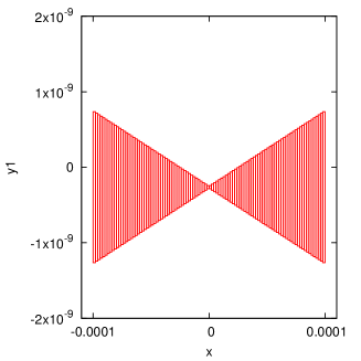
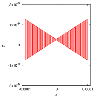
Figure 5: The projection onto $x,y_{1}$ coordinates of the bounds on $W_{G}^{u}$. On the left we have the bound for $G=G_{l}$ (the left end of our parameter interval (33)), and on the right for $G=G_{r}$.

To establish the bounds for the stable manifold, we consider the vector field with reversed sign (which makes the stable manifold become unstable), and apply Theorem 16 once again. Here we have obtained a Lipschitz bound $L_{s}=10^{-3}$. In Figure 6 we see the bound on the enclosure. The two points on the plot are the $\Phi_{T}\left(p_{G}^{u},G\right)$ for $G=G_{l}$ and $G=G_{r}$ for the choice of $T=50$ (see (12) for the definition of $p_{G}^{u}$). We do not plot these as boxes, since our computer assisted bound gives their size of order $10^{-13},$ and such boxes would be invisible on the plot. Note that Figure 6 corresponds to the sketch from Figure 3. In Figure 6 we have the projection onto $x,y_{1}$ coordinates of what happens inside of the set $D$, without plotting the trajectory along the unstable manifold.

We use the rigorous estimates for $\Phi_{T}\left(p_{G_{l}}^{u},G_{l}\right)$ and $\Phi_{T}\left(p_{G_{r}}^{u},G_{r}\right)$ to compute the following bounds (see (13) for the definition of the function $h$,)

$$h\left(G_{l}\right) \in[1.193520892609e-07,1.2017042212622e-07],$$

$$h\left(G_{l}\right) \in\left[-1.1920396632516e-07,-1.1838527119022e-07\right].$$

We also make sure that $\Phi_{T}\left(p_{G}^{u},G\right)\in D$ for all $G\in[G_{l},G_{r}]$. We see that assumption (14) of Theorem 10 is satisfied, which means that we have a Shil’nikov homoclinic connection for at least one of the parameters $G\in\left[G_{l},G_{r}\right]$.

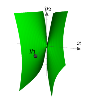
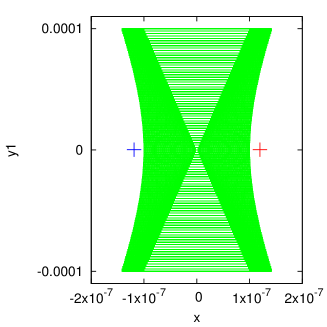
Figure 6: The bound on $W_{G}^{s}$, for all parameters $G$ from (33). On the left we have a non-rigorous plot, to illustrate the shape of our bound in three dimensions. On the right, we have a projection onto the $x,y_{1}$ coordinates of the rigorous, computer assisted enclosure. The two points depicted on the right hand side plot are $\Phi_{T}\left(p_{G_{l}}^{u},G_{l}\right)$ (on the right, in red) and $\Phi_{T}\left(p_{G_{r}}^{u},G_{r}\right)$ (on the left, in blue).

To establish the bound on $h^{\prime}\left(G\right)$, we first use Theorem 18 to establish an estimate for $\frac{d}{dG}w^{u}\left(x,G\right)$. In our computer assisted proof we use Theorem 18 with parameter $M=M_{u}:=2000$. We then use Theorem 18 once again to establish bounds for $\frac{d}{dG}w^{s}\left(x,G\right)$. (Here, again, we reverse the sign of the vector field to make the manifold unstable.) We establish the bound with $M_{s}=500.$ We then propagate the bound for $\frac{d}{dG}w^{u}\left(x,G\right)$ using rigorous, computer assisted integration, to obtain the bound

$$h^{\prime}\left(G\right)\in\left[-36.12,-34.57\right],\qquad\text{for all }G\in\left[G_{l},G_{r}\right].$$

This, by Theorem 10, establishes the uniqueness of the intersection parameter in $\left[G_{l},G_{r}\right]$.

Remark 21

We do not rule out a possiblility that for some parameter $G\in\left[G_{l},G_{r}\right]$ the trajectory $\Phi_{t}\left(p_{G}^{u},G\right)$ could exit $D$ and return again to intersect $W_{G}^{s}$. We have not done such investigation, which would require a global consideration of the system. What we establish is that we have a single parameter for which the homoclinic orbit behaves as the one in Figure 1.

The computer assisted proof has been done entirely by using the CAPD package and took 4 seconds on a single core 3Ghz Intel i7 processor.

8 Appendix

Proof of Lemma 2. Let us take any $t>0$ and any $p,q\in\mathbb{R}^{n}$ such that $\{\Phi_{-s}(p),\Phi_{-s}(q):s\in[0,t]\}\subset U$. Observe that since $U$ is convex, for any $u\in[0,1],$

$$Df\left(q+u\left(p-q\right)\right)\in[Df(U)].$$

Moreover,

$$f\left(p\right)-f\left(q\right)=\int_{0}^{1}Df\left(q+u\left(p-q\right)\right)du\left(p-q\right).$$

Using this we have

$$\Phi_{-t}\left(p\right)-\Phi_{-t}\left(q\right)$$

$$=p-q-\int_{0}^{t}f\left(\Phi_{-s}\left(p\right)\right)-f\left(\Phi_{-s}\left(q\right)\right)ds$$

$$=p-q$$

$$\ -\int_{0}^{t}\int_{0}^{1}Df\left(\Phi_{-s}\left(q\right)+u\left(\Phi_{-s}\left(p\right)-\Phi_{-s}\left(q\right)\right)\right)du\left(\Phi_{-s}\left(p\right)-\Phi_{-s}\left(q\right)\right)ds$$

$$=p-q-\int_{0}^{t}C(s)\left(\Phi_{-s}\left(p\right)-\Phi_{-s}\left(q\right)\right)ds,$$ (34)

where $\{C(s)\}$ is a family of matrixes defined as

$$C(s)=\int_{0}^{1}Df\left(\Phi_{-s}\left(q\right)+u\left(\Phi_{-s}\left(p\right)-\Phi_{-s}\left(q\right)\right)\right)du\in\left[Df\left(U\right)\right].$$

Since $f$ is $C^{1}$ in $U$ and $U$ is compact, there exists a constant $L>0$ such that for any $p\in U$

$$\left\|Df(p)\right\|\leq L.$$

Using standard Gronwall estimates gives that

$$\Phi_{-s}\left(p\right)-\Phi_{-s}\left(q\right)=p-q+h\left(s,p,q\right),$$ (35)

where $h$ satisfies

$$\left\|h\left(s,p,q\right)\right\|\leq\left(e^{sL}-1\right)\left\|p-q\right\|.$$

We can return to (34) and substitute (35) into the term under the integral to obtain

$$\Phi_{-t}\left(p\right)-\Phi_{-t}\left(q\right) =p-q-\int_{0}^{t}C(s)\left(p-q+h\left(s,p,q\right)\right)ds$$

$$=p-q-tC\left(p-q\right)+g\left(t,p,q\right),$$

for

$$C:=\frac{1}{t}\int_{0}^{t}C(s)ds\in\left[Df\left(U\right)\right],$$

and

$$g\left(t,p,q\right):=-\int_{0}^{t}C(s)h\left(s,p,q\right)ds.$$

Observing that

$$\left\|g\left(t,p,q\right)\right\| \leq\max_{s\in\left[0,t\right]}\left\|C\left(s\right)\right\|\left\|p-q\right\|\int_{0}^{t}\left(e^{sL}-1\right)ds$$

$$=\max_{s\in\left[0,t\right]}\left\|C\left(s\right)\right\|\left\|p-q\right\|\frac{1}{L}\left(e^{Lt}-Lt-1\right)$$

$$\leq M\left\|p-q\right\|t^{2},$$

gives the claim.

References

- [1] G. Alefeld, Inclusion methods for systems of nonlinear equations - the interval Newton method and modifications. Topics in validated computations (Oldenburg, 1993), 7–26, Stud. Comput. Math., 5, North-Holland, Amsterdam, 1994.
- [2] H. W. Broer, C. Simó, R. Vitolo, Bifurcations and strange attractors in the Lorenz-84 climate model with seasonal forcing, Nonlinearity, 15 (2002), 1205-1267.
- [3] M.J. Capiński, P. Zgliczyński, Beyond the Melnikov method: a computer assisted approach, preprint: http://arxiv.org/abs/1603.07131
- [4] M.J. Capiński, P. Zgliczyński, Geometric proof for normally hyperbolic invariant manifolds, J. Differential Equations 259 (2015) 6215–6286.
- [5] G. Dahlquist, Stability and Error Bounds in the Numerical Intgration of Ordinary Differential Equations, Almqvist & Wiksells, Uppsala, 1958; Transactions of the Royal Institute of Technology, Stockholm, 1959.
- [6] N. Fenichel. Persistence and smoothness of invariant manifolds for flows. Indiana Univ. Math. J., 21:193–226, 1971/1972.
- [7] N. Fenichel. Asymptotic stability with rate conditions. Indiana Univ. Math. J., 23: 1109–1137, 1973/74.
- [8] N. Fenichel. Asymptotic stability with rate conditions for dynamical systems. Bull. Amer. Math. Soc., 80:346–349, 1974.
- [9] N. Fenichel. Asymptotic stability with rate conditions. II. Indiana Univ. Math. J., 26(1):81–93, 1977.
- [10] M. Gidea, P. Zgliczyński, Covering relations for multidimensional dynamical systems I, J. of Diff. Equations 202(2004) 32–58
- [11] M. Gidea, P. Zgliczyński, Covering relations for multidimensional dynamical systems II, J. of Diff. Equations 202(2004) 59–80
- [12] E. Hairer, S.P. Nørsett and G. Wanner, Solving Ordinary Differential Equations I, Nonstiff Problems, Springer-Verlag, Berlin Heidelberg 1987.
- [13] P. Hartman, Ordinary differential equations. Corrected reprint. S. M. Hartman, Baltimore, Md., 1973.
- [14] M. W. Hirsch, C. C. Pugh, M. Shub, Invariant manifolds. Lecture Notes in Mathematics, Vol. 583. Springer-Verlag, Berlin-New York, 1977.
- [15] Y. Kuznetsov, Elements of Applied Bifurcation Theory, 1995, New York:Springer.
- [16] T. Kapela and P. Zgliczyński, A Lohner-type algorithm for control systems and ordinary differential inclusions, Discrete Cont. Dyn. Sys. B, vol. 11(2009), 365-385.
- [17] E.N. Lorenz, Irregularity: a fundamental property of the atmosphere, Tellus Series A-dynamic Meteorology and Oceanography vol. 36A (1984), no. 2, 98–110.
- [18] E.N. Lorenz, Can chaos and intransitivity lead to interannual variability?, Tellus Series A-dynamic Meteorology and Oceanography vol. 42A (1990), 378–389.
- [19] S. M. Lozinskii, Error esitimates for the numerical integration of ordinary differential equations, part I, Izv. Vyss. Uceb. Zaved. Matematica,6 (1958), 52–90 (Russian)
- [20] Z. Nitecki, Differentiable dynamics. An introduction to the orbit structure of diffeomorphisms. The M.I.T. Press, Cambridge, 1971.
- [21] L.P. Shil’nikov, A case of the existence of a denumerable set of periodic motions, Soviet Mathematics - Doklady 6 (1965), 163–166.
- [22] L.P. Shil’nikov, The existence of a countable set of periodic motions in the neighborhood of a homoclinic curve, Soviet Mathematics - Doklady 8 (1967), 102-106.
- [23] L.P. Shil’nikov, A contribution to the problem of the structure of an extended neighborhood of a rough equilibrium state of a saddle-focus type, Mathematics of the USSR. Sbornik 10 (1970), 91–102.
- [24] L.P. Shil’nikov, A.L. Shil’nikov, D.V. Turaev, L.O. Chua, Methods of Qualitative Theory in Nonlinear Dynamics: (Part II), World Scientific Series on Nonlinear Science Series A, (2001),
- [25] A. Shil’nikov, G. Nicolis, C. Nicolis Bifurcation and predictability analysis of a low-order atmospheric circulation model, International Journal of Bifurcation and Chaos 5 (1995), 1701–1711
- [26] G. Tigan, D. Turaev Analytical search for homoclinic bifurcations in the Shimizu-Morioka model Physica D, 240 (2011) 985–989
- [27] L. van Veen, Baroclinic flow and the Lorenz-84 model. International Journal of Bifurcation and Chaos 13 (08) (2003), 2117–2139.
- [28] D. Wilczak, The existence of Shilnikov homoclinic orbits in the Michelson system: a computer assisted proof. Foundations of Computational Mathematics, Vol.6, No.4, 495–535, (2006).