Integrating Distributional Lexical Contrast into Word Embeddings for Antonym–Synonym Distinction

Abstract

We propose a novel vector representation that integrates lexical contrast into distributional vectors and strengthens the most salient features for determining degrees of word similarity. The improved vectors significantly outperform standard models and distinguish antonyms from synonyms with an average precision of 0.66–0.76 across word classes (adjectives, nouns, verbs). Moreover, we integrate the lexical contrast vectors into the objective function of a skip-gram model. The novel embedding outperforms state-of-the-art models on predicting word similarities in SimLex-999, and on distinguishing antonyms from synonyms.

1 Introduction

Antonymy and synonymy represent lexical semantic relations that are central to the organization of the mental lexicon [Miller and Fellbaum, 1991]. While antonymy is defined as the oppositeness between words, synonymy refers to words that are similar in meaning [Deese, 1965, Lyons, 1977]. From a computational point of view, distinguishing between antonymy and synonymy is important for NLP applications such as Machine Translation and Textual Entailment, which go beyond a general notion of semantic relatedness and require to identify specific semantic relations. However, due to interchangeable substitution, antonyms and synonyms often occur in similar contexts, which makes it challenging to automatically distinguish between them.

Distributional semantic models (DSMs) offer a means to represent meaning vectors of words and to determine their semantic “relatedness” [Budanitsky and Hirst, 2006, Turney and Pantel, 2010]. They rely on the distributional hypothesis [Harris, 1954, Firth, 1957], in which words with similar distributions have related meaning. For computation, each word is represented by a weighted feature vector, where features typically correspond to words that co-occur in a particular context. However, DSMs tend to retrieve both synonyms (such as formal–conventional) and antonyms (such as formal–informal) as related words and cannot sufficiently distinguish between the two relations.

In recent years, a number of distributional approaches have accepted the challenge to distinguish antonyms from synonyms, often in combination with lexical resources such as thesauruses or taxonomies. For example, ?) used dependency triples to extract distributionally similar words, and then in a post-processing step filtered out words that appeared with the patterns ‘from X to Y’ or ‘either X or Y’ significantly often. ?) assumed that word pairs that occur in the same thesaurus category are close in meaning and marked as synonyms, while word pairs occurring in contrasting thesaurus categories or paragraphs are marked as opposites. ?) showed that the distributional difference between antonyms and synonyms can be identified via a simple word space model by using appropriate features. ?) and ?) aimed to identify the most salient dimensions of meaning in vector representations and reported a new average-precision-based distributional measure and an entropy-based measure to discriminate antonyms from synonyms (and further paradigmatic semantic relations).

Lately, antonym–synonym distinction has also been a focus of word embedding models. For example, ?) integrated coreference chains extracted from large corpora into a skip-gram model to create word embeddings that identified antonyms. ?) proposed thesaurus-based word embeddings to capture antonyms. They proposed two models: the WE-T model that trains word embeddings on thesaurus information; and the WE-TD model that incorporated distributional information into the WE-T model. ?) introduced the multitask lexical contrast model (mLCM) by incorporating WordNet into a skip-gram model to optimize semantic vectors to predict contexts. Their model outperformed standard skip-gram models with negative sampling on both general semantic tasks and distinguishing antonyms from synonyms.

In this paper, we propose two approaches that make use of lexical contrast information in distributional semantic space and word embeddings for antonym–synonym distinction. Firstly, we incorporate lexical contrast into distributional vectors and strengthen those word features that are most salient for determining word similarities, assuming that feature overlap in synonyms is stronger than feature overlap in antonyms. Secondly, we propose a novel extension of a skip-gram model with negative sampling [Mikolov et al., 2013b] that integrates the lexical contrast information into the objective function. The proposed model optimizes the semantic vectors to predict degrees of word similarity and also to distinguish antonyms from synonyms. The improved word embeddings outperform state-of-the-art models on antonym–synonym distinction and a word similarity task.

2 Our Approach

In this section, we present the two contributions of this paper: a new vector representation that improves the quality of weighted features to distinguish between antonyms and synonyms (Section 2.1), and a novel extension of skip-gram models that integrates the improved vector representations into the objective function, in order to predict similarities between words and to identify antonyms (Section 2.2).

2.1 Improving the weights of feature vectors

We aim to improve the quality of weighted feature vectors by strengthening those features that are most salient in the vectors and by putting less emphasis on those that are of minor importance, when distinguishing degrees of similarity between words. We start out with standard corpus co-occurrence frequencies and apply local mutual information (LMI) [Evert, 2005] to determine the original strengths of the word features. Our score $weight^{SA}(w,f)$ subsequently defines the weights of a target word $w$ and a feature $f$:

The new $weight^{SA}$ scores of a target word $w$ and a feature $f$ exploit the differences between the average similarities of synonyms to the target word ($sim(w,u)$, with $u\in S(w)$), and the average similarities between antonyms of the target word ($sim(w^{\prime},v)$, with $w^{\prime}\in A(w)$ and $v\in S(w^{\prime})$). Only those words $u$ and $v$ are included in the calculation that have a positive original LMI score for the feature $f$: $W(f)$. To calculate the similarity $sim$ between two word vectors, we rely on cosine distances. If a word $w$ is not associated with any synonyms or antonyms in our resources (cf. Section 3.1), or if a feature does not co-occur with a word $w$, we define $weight^{SA}(w,f)=0$.

The intuition behind the lexical contrast information in our new $weight^{SA}$ is as follows. The strongest features of a word also tend to represent strong features of its synonyms, but weaker features of its antonyms. For example, the feature conception only occurs with synonyms of the adjective formal but not with the antonym informal, or with synonyms of the antonym informal. $weight^{SA}(formal,conception)$, which is calculated as the average similarity between formal and its synonyms minus the average similarity between informal and its synonyms, should thus return a high positive value. In contrast, a feature such as issue that occurs with many different adjectives, would enforce a feature score near zero for $weight^{SA}(formal,issue)$, because the similarity scores between formal and its synonyms and informal and its synonyms should not differ strongly. Last but not least, a feature such as rumor that only occurs with informal and its synonyms, but not with the original target adjective formal and its synonyms, should invoke a very low value for $weight^{SA}(formal,rumor)$. Figure 1 provides a schematic visualization for computing the new $weight^{SA}$ scores for the target formal.

Since the number of antonyms is usually much smaller than the number of synonyms, we enrich the number of antonyms: Instead of using the direct antonym links, we consider all synonyms of an antonym $w^{\prime}\in A(w)$ as antonyms of $w$. For example, the target word good has only two antonyms in WordNet (bad and evil), in comparison to 31 synonyms. Thus, we also exploit the synonyms of bad and evil as antonyms for good.

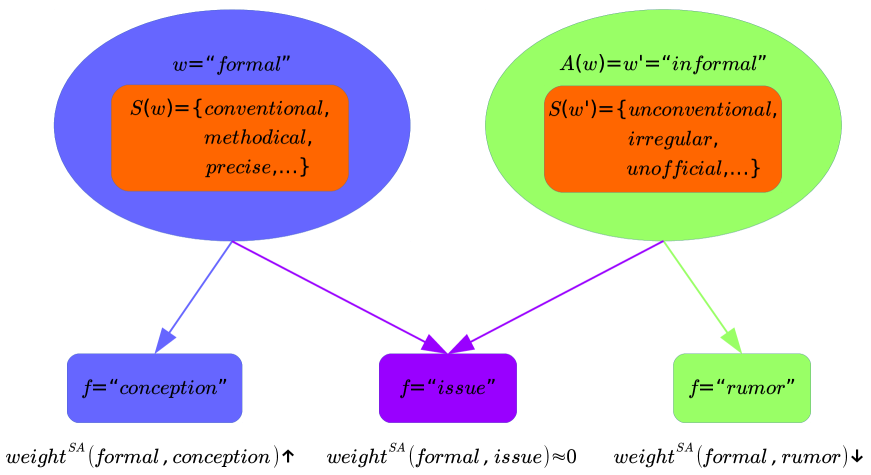
Figure 1: Illustration of the $weight^{SA}$ scores for the adjective target formal. The feature conception only occurs with formal and synonyms of formal, so $weight^{SA}(formal,conception)$ should return a positive value; the feature rumor only occurs with the antonym informal and with synonyms of informal, so $weight^{SA}(formal,rumor)$ should return a negative value; the feature issue occurs with both formal and informal and also with synonyms of these two adjectives, so $weight^{SA}(formal,issue)$ should return a feature score near zero.

2.2 Integrating the distributional lexical contrast into a skip-gram model

Our model relies on Levy and Goldberg [Levy and Goldberg, 2014] who showed that the objective function for a skip-gram model with negative sampling (SGNS) can be defined as follows:

$$\begin{array}[]{l}\sum\limits_{w\in V}{\sum\limits_{c\in V}\{}\#(w,c)\log\sigma(sim(w,c))\\ +k\#(w){P_{0}}(c)\log\sigma(-sim(w,c))\}\end{array}$$ (2)

The first term in Equation (2) represents the co-occurrence between a target word $w$ and a context $c$ within a context window. The number of appearances of the target word and that context is defined as $\#(w,c)$. The second term refers to the negative sampling where $k$ is the number of negatively sampled words, and $\#(w)$ is the number of appearances of $w$ as a target word in the unigram distribution $P_{0}$ of its negative context $c$.

To incorporate our lexical contrast information into the SGNS model, we propose the objective function in Equation (3) to add distributional contrast followed by all contexts of the target word. $V$ is the vocabulary; $\sigma(x)=\frac{1}{{1+{e^{-x}}}}$ is the sigmoid function; and $sim(w_{1},w_{2})$ is the cosine similarity between the two embedded vectors of the corresponding two words $w_{1}$ and $w_{2}$. We refer to our distributional lexical-contrast embedding model as dLCE.

$$\begin{array}[]{l}\sum\limits_{w\in V}{\sum\limits_{c\in V}\{}(\#(w,c)\log\sigma(sim(w,c))\\ +k\#(w){P_{0}}(c)\log\sigma(-sim(w,c)))\\ +(\frac{1}{{\#(w,u)}}\sum\nolimits_{u\in W(c)\cap S(w)}{sim(w,u)}\\ -\frac{1}{{\#(w,v)}}\sum\nolimits_{v\in W(c)\cap A(w)}{sim(w,v)})\}\end{array}$$ (3)

Equation (3) integrates the lexical contrast information in a slightly different way compared to Equation (1): For each of the target words $w$, we only rely on its antonyms $A(w)$ instead of using the synonyms of its antonyms $S(w^{\prime})$. This makes the word embeddings training more efficient in running time, especially since we are using a large amount of training data.

The dLCE model is similar to the WE-TD model [Ono et al., 2015] and the mLCM model [Pham et al., 2015]; however, while the WE-TD and mLCM models only apply the lexical contrast information from WordNet to each of the target words, dLCE applies lexical contrast to every single context of a target word in order to better capture and classify semantic contrast.

	Adjectives		Nouns		Verbs
	ANT	SYN	ANT	SYN	ANT	SYN
LMI	0.46	0.56	0.42	0.60	0.42	0.62
$weight^{SA}$	0.36∗∗	0.75∗∗	0.40	0.66	0.38∗	0.71∗
LMI + SVD	0.46	0.55	0.46	0.55	0.44	0.58
$weight^{SA}$ + SVD	0.36∗∗∗	0.76∗∗∗	0.40∗	0.66∗	0.38∗∗∗	0.70∗∗∗

Table 1: AP evaluation on DSMs.

3 Experiments

3.1 Experimental Settings

The corpus resource for our vector representations is one of the currently largest web corpora: ENCOW14A [Schäfer and Bildhauer, 2012, Schäfer, 2015], containing approximately 14.5 billion tokens and 561K distinct word types. As distributional information, we used a window size of 5 tokens for both the original vector representation and the word embeddings models. For word embeddings models, we trained word vectors with 500 dimensions; $k$ negative sampling was set to 15; the threshold for sub-sampling was set to $10^{-5}$; and we ignored all words that occurred $<100$ times in the corpus. The parameters of the models were estimated by backpropagation of error via stochastic gradient descent. The learning rate strategy was similar to Mikolov et al. [Mikolov et al., 2013a] in which the initial learning rate was set to 0.025. For the lexical contrast information, we used WordNet [Miller, 1995] and Wordnik to collect antonyms and synonyms, obtaining a total of 363,309 synonym and 38,423 antonym pairs.

3.2 Distinguishing antonyms from synonyms

The first experiment evaluates our lexical contrast vectors by applying the vector representations with the improved $weight^{SA}$ scores to the task of distinguishing antonyms from synonyms. As gold standard resource, we used the English dataset described in [Roth and Schulte im Walde, 2014], containing 600 adjective pairs (300 antonymous pairs and 300 synonymous pairs), 700 noun pairs (350 antonymous pairs and 350 synonymous pairs) and 800 verb pairs (400 antonymous pairs and 400 synonymous pairs). For evaluation, we applied Average Precision (AP) [Voorhees and Harman, 1999], a common metric in information retrieval previously used by ?) and ?), among others.

Table 1 presents the results of the first experiment, comparing our improved vector representations with the original LMI representations across word classes, without/with applying singular-value decomposition (SVD), respectively. In order to evaluate the distribution of word pairs with AP, we sorted the synonymous and antonymous pairs by their cosine scores. A synonymous pair was considered correct if it belonged to the first half; and an antonymous pairs was considered correct if it was in the second half. The optimal results would thus achieve an AP score of 1 for $SYN$ and 0 for $ANT$. The results in the tables demonstrate that $weight^{SA}$ significantly outperforms the original vector representations across word classes.

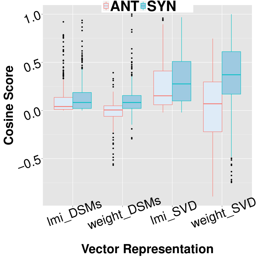
(a) Cosine scores between adjectives.

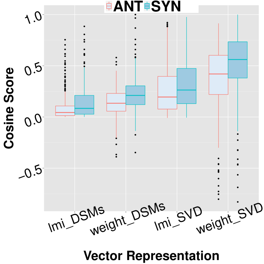
(b) Cosine scores between nouns.

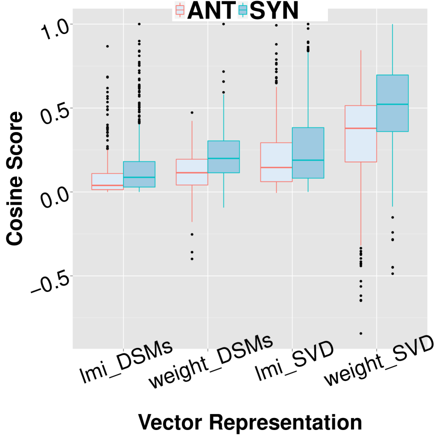
(c) Cosine scores between verbs.

Figure 2: Differences between cosine scores for antonymous vs. synonymous word pairs.

In addition, Figure 2 compares the medians of cosine similarities between antonymous pairs (red) vs. synonymous pairs (green) across word classes, and for the four conditions (1) LMI, (2) $weight^{SA}$, (3) SVD on LMI, and (4) SVD on $weight^{SA}$. The plots show that the cosine similarities of the two relations differ more strongly with our improved vector representations in comparison to the original LMI representations, and even more so after applying SVD.

3.3 Effects of distributional lexical contrast on word embeddings

The second experiment evaluates the performance of our dLCE model on both antonym–synonym distinction and a word similarity task. The similarity task requires to predict the degree of similarity for word pairs, and the ranked list of predictions is evaluated against a gold standard of human ratings, relying on the Spearman rank-order correlation coefficient $\rho$ [Siegel and Castellan, 1988].

In this paper, we use the SimLex-999 dataset [Hill et al., 2015] to evaluate word embedding models on predicting similarities. The resource contains 999 word pairs (666 noun, 222 verb and 111 adjective pairs) and was explicitly built to test models on capturing similarity rather than relatedness or association. Table 2 shows that our dLCE model outperforms both SGNS and mLCM, proving that the lexical contrast information has a positive effect on predicting similarity.

Therefore, the improved distinction between synonyms (strongly similar words) and antonyms (often strongly related but highly dissimilar words) in the dLCE model also supports the distinction between degrees of similarity.

SGNS	mLCM	dLCE
0.38	0.51	0.59

Table 2: Spearman’s $\rho$ on SimLex-999.

For distinguishing between antonyms and synonyms, we computed the cosine similarities between word pairs on the dataset described in Section 3.2, and then used the area under the ROC curve (AUC) to evaluate the performance of dLCE compared to SGNS and mLCM. The results in Table 3 report that dLCE outperforms SGNS and mLCM also on this task.

	Adjectives	Nouns	Verbs
SGNS	0.64	0.66	0.65
mLCM	0.85	0.69	0.71
dLCE	0.90	0.72	0.81

Table 3: AUC scores for identifying antonyms.

4 Conclusion

This paper proposed a novel vector representation which enhanced the prediction of word similarity, both for a traditional distributional semantics model and word embeddings. Firstly, we significantly improved the quality of weighted features to distinguish antonyms from synonyms by using lexical contrast information. Secondly, we incorporated the lexical contrast information into a skip-gram model to successfully predict degrees of similarity and also to identify antonyms.

References

- [Adel and Schütze, 2014] Heike Adel and Hinrich Schütze. 2014. Using mined coreference chains as a resource for a semantic task. In Proceedings of the 2014 Conference on Empirical Methods in Natural Language Processing, pages 1447–1452, Doha, Qatar.
- [Budanitsky and Hirst, 2006] Alexander Budanitsky and Graeme Hirst. 2006. Evaluating WordNet-based measures of lexical semantic relatedness. Computational Linguistics, 32(1):13–47.
- [Deese, 1965] James Deese. 1965. The Structure of Associations in Language and Thought. The John Hopkins Press, Baltimore, MD.
- [Evert, 2005] Stefan Evert. 2005. The Statistics of Word Cooccurrences. Ph.D. thesis, Stuttgart University.
- [Firth, 1957] John R. Firth. 1957. Papers in Linguistics 1934-51. Longmans, London, UK.
- [Harris, 1954] Zellig S. Harris. 1954. Distributional structure. Word, 10(23):146–162.
- [Hill et al., 2015] Felix Hill, Roi Reichart, and Anna Korhonen. 2015. Simlex-999: Evaluating semantic models with (genuine) similarity estimation. Computational Linguistics, 41(4):665–695.
- [Kotlerman et al., 2010] Lili Kotlerman, Ido Dagan, Idan Szpektor, and Maayan Zhitomirsky-Geffet. 2010. Directional distributional similarity for lexical inference. Natural Language Processing, 16(4):359–389.
- [Levy and Goldberg, 2014] Omer Levy and Yoav Goldberg. 2014. Neural word embedding as implicit matrix factorization. In Z. Ghahramani, M. Welling, C. Cortes, N.D. Lawrence, and K.Q. Weinberger, editors, Advances in Neural Information Processing Systems 27, pages 2177–2185.
- [Lin et al., 2003] Dekang Lin, Shaojun Zhao, Lijuan Qin, and Ming Zhou. 2003. Identifying synonyms among distributionally similar words. In Proceedings of the 18th International Joint Conference on Artificial Intelligence, pages 1492–1493, Acapulco, Mexico.
- [Lyons, 1977] John Lyons. 1977. Semantics, volume 1. Cambridge University Press.
- [Mikolov et al., 2013a] Tomas Mikolov, Kai Chen, Greg Corrado, and Jeffrey Dean. 2013a. Efficient estimation of word representations in vector space. Computing Research Repository, abs/1301.3781.
- [Mikolov et al., 2013b] Tomas Mikolov, Wen-tau Yih, and Geoffrey Zweig. 2013b. Linguistic regularities in continuous space word representations. In Proceedings of the Conference of the North American Chapter of the Association for Computational Linguistics: Human Language Technologies, pages 746–751, Atlanta, Georgia.
- [Miller and Fellbaum, 1991] George A. Miller and Christiane Fellbaum. 1991. Semantic networks of English. Cognition, 41:197–229.
- [Miller, 1995] George A. Miller. 1995. WordNet: A lexical database for English. Communications of the ACM, 38(11):39–41.
- [Mohammad et al., 2013] Saif M. Mohammad, Bonnie J. Dorr, Graeme Hirst, and Peter D. Turney. 2013. Computing lexical contrast. Computational Linguistics, 39(3):555–590.
- [Ono et al., 2015] Masataka Ono, Makoto Miwa, and Yutaka Sasaki. 2015. Word embedding-based antonym detection using thesauri and distributional information. In Proceedings of the Conference of the North American Chapter of the Association for Computational Linguistics: Human Language Technologies, pages 984–989, Denver, Colorado.
- [Pham et al., 2015] Nghia The Pham, Angeliki Lazaridou, and Marco Baroni. 2015. A multitask objective to inject lexical contrast into distributional semantics. In Proceedings of the 53rd Annual Meeting of the Association for Computational Linguistics and the 7th International Joint Conference on Natural Language Processing, pages 21–26, Beijing, China.
- [Roth and Schulte im Walde, 2014] Michael Roth and Sabine Schulte im Walde. 2014. Combining word patterns and discourse markers for paradigmatic relation classification. In Proceedings of the 52nd Annual Meeting of the Association for Computational Linguistics, pages 524–530, Baltimore, MD.
- [Santus et al., 2014a] Enrico Santus, Alessandro Lenci, Qin Lu, and Sabine Schulte im Walde. 2014a. Chasing hypernyms in vector spaces with entropy. In Proceedings of the 14th Conference of the European Chapter of the Association for Computational Linguistics, pages 38–42, Gothenburg, Sweden.
- [Santus et al., 2014b] Enrico Santus, Qin Lu, Alessandro Lenci, and Chu-Ren Huang. 2014b. Taking antonymy mask off in vector space. In Proceedings of the 28th Pacific Asia Conference on Language, Information and Computation, pages 135–144.
- [Schäfer and Bildhauer, 2012] Roland Schäfer and Felix Bildhauer. 2012. Building large corpora from the web using a new efficient tool chain. In Proceedings of the 8th International Conference on Language Resources and Evaluation, pages 486–493, Istanbul, Turkey.
- [Schäfer, 2015] Roland Schäfer. 2015. Processing and querying large web corpora with the COW14 architecture. In Proceedings of the 3rd Workshop on Challenges in the Management of Large Corpora, pages 28–34.
- [Scheible et al., 2013] Silke Scheible, Sabine Schulte im Walde, and Sylvia Springorum. 2013. Uncovering distributional differences between synonyms and antonyms in a word space model. In Proceedings of the 6th International Joint Conference on Natural Language Processing, pages 489–497, Nagoya, Japan.
- [Siegel and Castellan, 1988] Sidney Siegel and N. John Castellan. 1988. Nonparametric Statistics for the Behavioral Sciences. McGraw-Hill, Boston, MA.
- [Turney and Pantel, 2010] Peter D. Turney and Patrick Pantel. 2010. From frequency to meaning: Vector space models of semantics. Journal of Artificial Intelligence Research, 37:141–188.
- [Voorhees and Harman, 1999] Ellen M. Voorhees and Donna K. Harman. 1999. The 7th Text REtrieval Conference (trec-7). National Institute of Standards and Technology, NIST.