Coherent magneto-elastic oscillations in superfluid magnetars

Abstract

We study the effect of superfluidity on torsional oscillations of highly magnetised neutron stars (magnetars) with a microphysical equation of state by means of two-dimensional, magneto-hydrodynamical-elastic simulations. The superfluid properties of the neutrons in the neutron star core are treated in a parametric way in which we effectively decouple part of the core matter from the oscillations. Our simulations confirm the existence of two groups of oscillations, namely continuum oscillations that are confined to the neutron star core and are of Alfvénic character, and global oscillations with constant phase and that are of mixed magneto-elastic type. The latter might explain the quasi-periodic oscillations observed in magnetar giant flares, since they do not suffer from the additional damping mechanism due to phase mixing, contrary to what happens for continuum oscillations. However, we cannot prove rigorously that the coherent oscillations with constant phase are normal modes. Moreover, we find no crustal shear modes for the magnetic field strengths typical for magnetars. We provide fits to our numerical simulations that give the oscillation frequencies as functions of magnetic field strength and proton fraction in the core.

1 Introduction

The analysis of the X-ray light curves of the giant flares of the soft gamma-ray repeaters (SGRs) SGR 1806-20 and SGR 1900+14 revealed a number of quasi-periodic oscillation (QPOs) with frequencies at $18$, $26$, $30$, $92$, $150$, $625$, $1840\,$Hz (SGR 1806-20) and $28$, $53$, $84$, $155$ Hz (SGR 1900+14) (see e.g. Israel et al., 2005; Strohmayer & Watts, 2005; Watts & Strohmayer, 2006; Strohmayer & Watts, 2006). The importance of this discovery became apparent when the observed QPOs were identified as oscillations of the neutron star. If such interpretation were true, it would provide a unique tool to study the interior of a neutron star through asteroseismology. Since the oscillation frequencies of a neutron star depend sensitively on the equation of state (EoS) the matching of a theoretical model with the observations would allow to constrain the EoS. More recent studies found additional QPOs in the flare of SGR 1806-20 (at $17$, $21$, $36$, $59$, and $116\,$Hz in Hambaryan et al., 2011) and also in less energetic bursts of SGR 1806-20 (at $57\,$Hz in Huppenkothen et al., 2014c) and in SGR J1550-5418 (at $93$, $127$, and $260\,$Hz in Huppenkothen et al., 2014a). The observed frequencies can thus be neatly divided into two groups, below $260\,$Hz and above $500\,$Hz.

Initially the observed QPO frequencies were assumed to be discrete torsional shear oscillations of the elastic crust of the neutron star. The low-frequency QPOs match approximately the frequencies of fundamental torsional crustal shear modes $t_{n}^{l}$, i.e. modes without nodes in the radial direction ($n=0$), while the higher frequencies could correspond to overtones ($n>0$). The model of shear modes has been investigated carefully by many groups and different aspects of the nuclear physics of the crust have been discussed in detail (see Duncan, 1998; Messios et al., 2001; Strohmayer & Watts, 2005; Piro, 2005; Sotani et al., 2007; Samuelsson & Andersson, 2007; Steiner & Watts, 2009; Deibel et al., 2014; Sotani et al., 2016, and references therein).

However, the observed properties of SGRs indicate that the problem is more difficult. Their X-ray luminosity, X-ray spectra, spin-down measurements and bursting activity together with other observational indications strongly suggest that SGRs are highly magnetised neutron stars (magnetars) with surface field strengths of up to $B\gtrsim 10^{15}\,$G (Duncan & Thompson, 1992). These strong magnetic fields lead to torsional Alfvén oscillations with frequencies around $30\,$Hz (Sotani et al., 2008; Cerdá-Durán et al., 2009; Colaiuda et al., 2009), exactly in the right frequency range of the observed QPO frequencies. The Alfvén oscillations do not form an eigenmode system but can be found as long-lived QPOs at the turning points and edges of an Alfvén ontinuum (Levin, 2007). For simplified models, it was shown by Levin (2006) and Glampedakis et al. (2006) that the interaction of the discrete crustal modes with the Alfvén continuum leads to strong absorption of the shear modes into the core. More realistic calculations confirmed this result and also showed that, instead of the crustal modes, magneto-elastic oscillations of predominantly Alfvénic character have frequencies that match the observed low-frequency QPOs. However, within this magneto-elastic model it is not easy to accommodate the highest observed QPO frequencies of $625$ and $1840\,$Hz (SGR 1806-20) (van Hoven & Levin, 2011; Gabler et al., 2011; Colaiuda & Kokkotas, 2011; van Hoven & Levin, 2012; Gabler et al., 2012). These would have to be fairly high overtones of the fundamental magneto-elastic oscillations, which would render problematic to explain why only such particular high-frequency QPOs are excited. In a more sophisticated analysis of the observations, Huppenkothen et al. (2014b) find that the data is consistent with the $625\,$Hz QPO being transient, which indicates a strong crust-core coupling.

Most of the above models considered a single fluid in the core of the neutron star, consisting of a mixture of neutrons, protons and electrons. This is a valid approach if the interactions between different species, such as neutrons and protons, are very strong. However, Migdal (1959) and Baym et al. (1969) discussed the possibility that the neutrons in the core of neutron stars are superfluid. This idea received strong support by Shternin et al. (2011) and Page et al. (2011) who showed that the cooling curve of Cas A is consistent with a phase transition to superfluid neutrons. If the neutrons are indeed superfluid, the matter in the core of neutron stars cannot be described within the single-fluid approach. First studies considering the effect of superfluid phases on the dynamics of the fluid mixture inside neutron stars (Mendell, 1991, 1998) were followed by Prix & Rieutord (2002); Andersson et al. (2002, 2004); Chamel (2008). These models provided the framework to obtain first estimates of the effects of superfluidity on the oscillation spectra of magnetised neutron stars without crust (Glampedakis et al., 2011; Passamonti & Lander, 2013). In particular, Passamonti & Lander (2013) tried to explain the high-frequency QPOs as Alfvén oscillations but had difficulties in identifying the low-frequency QPOs. Additionally, Samuelsson & Andersson (2009) and Sotani et al. (2013) investigated the effect of superfluid neutrons in the crust on the shear oscillations of the latter, but did not take magnetic fields into account.

The first magneto-elastic models considering superfluid effects were presented in Levin (2007); van Hoven & Levin (2008, 2011, 2012). These authors did not find significant differences from models without superfluidity other than a shift of the fundamental magneto-elastic frequency for a given magnetic field strength to higher values, however, which is important to bring the estimated magnetic field strength in agreement to those observed from spin-down measurements $\bar{B}\sim 10^{15}\,$G van Hoven & Levin (2008). Subsequent work by Gabler et al. (2013a) revealed that the inclusion of superfluid effects does not only modify the frequencies (such that the spin-down estimates for the global magnetic field strength are in better agreement with QPOs originating from magneto-elastic oscillations), but also that there exists a different type of QPOs that exhibit a constant phase throughout the star. Additionally, Gabler et al. (2013a) discovered high frequency oscillations that may explain the observed QPOs at $625$ and $1840\,$Hz. These results were confirmed in a study by Passamonti & Lander (2014). The evolutionary paths of the different (superfluid) magneto-elastic oscillations in magnetars were also analysed using order-of-magnitude estimates of different damping time scales in Glampedakis & Jones (2014).

In this work we extend the study initiated in Gabler et al. (2013a) and discuss in detail the effects of superfluidity on the spectrum of magneto-elastic oscillations of magnetars. We first review in Section 2 the equations for magneto-elastic oscillations in the single-fluid approach and then generalize these equations to the case of superfluid neutrons. We also update the equilibrium model used in Gabler et al. (2013a) with a magnetic field configuration that takes superfluid neutrons into account and discuss the boundary conditions for the simulations. In Section 3, we discuss the effects of superfluid neutrons on the low-frequency magneto-elastic oscillations. We confirm the existence of a new class of coherent oscillations with constant phases (Gabler et al., 2013a; Passamonti & Lander, 2014) and are able to distinguish two families: predominantly Alfvén QPOs that are confined to the core and have a continuous phase, and global magneto-elastic oscillations that have a constant phase. Then, we cast our ignorance about the superfluid entrainment factor and the proton fraction into one effective parameter and study the effects of a change of the latter. Finally, we discuss our results in Section 5.

Throughout this work we will use units where $c=G=1$, where, $c$ and $G$ are the speed of light and the gravitational constant, respectively. Latin (Greek) indices run from 1 to 3 (0 to 3). Partial derivatives are indicated by a comma and we apply the Einstein summation convention. The magnetic field strength we use is that of a uniformly magnetised rotating sphere with a radius of $10\,$km that would cause the same magnetic dipole spin-down as our stellar model (see Section 2.4 for details).

2 Theoretical framework

2.1 Evolution equations

This study is based on the numerical code MCOCOA that solves the general-relativistic magneto-hydrodynamical (GRMHD) equations and includes a description for elasticity. The implementation of GRMHD was discussed and tested carefully in Cerdá-Durán et al. (2008, 2009) and the treatment of elasticity was included in Gabler et al. (2011, 2012, 2013b). We assume a spherically symmetric spacetime, keep the space time fixed (Cowling approximation), and use the corresponding line element in isotropic coordinates

$$ds^{2}=-\alpha^{2}dt^{2}+\Phi^{4}\hat{\gamma}_{ij}dx^{i}dx^{j},\$$ (1)

where $\alpha$ and $\Phi$ are the lapse function and the conformal factor, respectively, and $\hat{\gamma}_{ij}={\rm diag}(1,r^{2},r^{2}\sin\theta)$ is the spatial, flat 3-metric. The circumferential radius $R$ is thus related to the coordinate radius $r$ by $R=\Phi^{2}r$.

The torsional magneto-elastic oscillations follow from the conservation of energy and momentum, baryon number conservation and Maxwell’s equations. If we further consider only linear perturbations in axisymmetry, poloidal and toroidal perturbations decouple and we can write down the following system of equations (Gabler et al., 2011, 2012):

$$\frac{1}{\sqrt{-g}}\left(\frac{\partial\sqrt{\gamma}\mathbf{U}}{\partial t}+\frac{\partial\sqrt{-g}\mathbf{F}^{i}}{\partial x^{i}}\right)=0\,,$$ (2)

where $g$ is the determinant of the metric, $\gamma$ is the determinant of the three-metric and the state vector $\bf U$ and flux vectors $\bf F^{i}$ are given by:

$$\mathbf{U} = [S_{\varphi},B^{\varphi}]\,,$$ (3)

$$\mathbf{F}^{r} = \left[-\frac{b_{\varphi}B^{r}}{W}-2\mu_{\mathrm{S}}\Sigma^{r}_{~{}\varphi},-v^{\varphi}B^{r}\right]\,,$$ (4)

$$\mathbf{F}^{\theta} = \left[-\frac{b_{\varphi}B^{\theta}}{W}-2\mu_{\mathrm{S}}\Sigma^{\theta}_{~{}\varphi},-v^{\varphi}B^{\theta}\right]\,.$$ (5)

Here, $B^{i}$ is the magnetic field measured by an Eulerian observer, $b_{i}$ that of a co-moving observer, $W=\alpha u^{t}$ the Lorentz factor, $v^{i}$ the three-velocity, $\mu_{\mathrm{S}}$ the shear modulus, $\Sigma^{\mu\nu}$ the shear tensor, and $S_{i}=(\rho h+b^{2})W^{2}v_{i}-\alpha b_{i}b^{0}$ is a generalisation of the momentum density, with $\rho$ and $h$ being the rest-mass density and specific enthalpy, respectively.

To solve these equations numerically, we need to know the two components of the shear tensor $\Sigma^{r}_{~{}\varphi}=g_{\varphi\varphi}g^{rr}\xi^{\varphi}_{,r}$ and $\Sigma^{\theta}_{~{}\varphi}=g_{\varphi\varphi}g^{\theta\theta}\xi^{\varphi}_{,\theta}$ that depend on the spatial derivatives of the displacement $\xi^{\varphi}$. The latter is related to the three velocity by

$$\xi^{j}_{\,,t}=\alpha v^{j}\,.$$ (6)

Because the order of the partial derivatives can be interchanged, we use the following equations for the spatial derivatives of $\xi^{\varphi}$

$$(\xi^{\varphi}_{\,,r})_{,t}-(v^{\varphi}\alpha)_{,r} = 0\,,$$ (7)

$$(\xi^{\varphi}_{\,,\theta})_{,t}-(v^{\varphi}\alpha)_{,\theta} = 0\,.$$ (8)

The complete system of equations of elastic GRMHD to be solved is given by Eqs. (2), (7) and (8) together with the corresponding definitions in Eqs.  (3)–(5). This set of equations assumes a single constituent fluid, i.e. all particles in the core respond together to any perturbation. However, theoretical (Baym et al., 1969) and observational (Anderson & Itoh, 1975; Shternin et al., 2011; Page et al., 2011) results indicate that neutrons are superfluid and protons are superconducting in old ($t\gtrsim 100$y) neutron star cores. In this work we consider magnetars with sufficiently strong magnetic fields ( $B\gtrsim\mathrm{few}\times 10^{15}\,$G at the surface and $B\sim 10^{16}\,$G in the core) to suppress the proton superconductivity in their cores (Glampedakis et al., 2011; Sinha & Sedrakian, 2015). As a result, and also because the MHD equations for superconducting protons (presently being developed by Graber et al., 2015) differ significantly from those of standard MHD, we neglect the effects of superconductivity and use the standard MHD equations.

For our neutron star models we assume a normal-matter EoS, i.e. we allow for neutrons, protons, electrons and muons. The latter three species are coupled together by the electromagnetic force. For the dynamics of this conglomerate the mass of the electrons (and muons) is negligible compared to that of the protons. Thus, we refer to all other constituents but superfluid neutrons as charged particles. In the crust the charged nuclei of the crustal lattice dominate the evolution instead of the protons. For the time scales considered here, the electrons and muons are assumed to co-move with the nuclei. Between the superfluid neutrons and the charged particles there is no direct interaction, i.e. the hydrodynamical equations of both fluids decouple. They interact with each other only through the gravitational potential. In contrast, in a mixture of superfluid neutrons and superconducting charged particles (protons) in the core, both superfluid components feel each other through the strong interaction and each of the superfluid species ‘entrains’ part of the other. For non-superconducting protons the corresponding entrainment coefficients $\varepsilon_{p}$ and $\varepsilon_{n}$ are zero (Gusakov & Haensel, 2005), where $n$ and $p$ denote neutrons and protons, respectively. The entrainment is related to the concept of effective mass $m^{\ast}$

$$\varepsilon_{x}=1-\frac{m^{\ast}_{x}}{m_{x}}\,,$$ (9)

where $m_{x}$ is the bare mass of the species $x\in\{n,~{}p\}$.

In Newtonian models, it was shown by Andersson et al. (2009) that the momentum equation of the neutrons for an incompressible fluid with constant background (which is equivalent to the assumption made for torsional oscillations) is coupled to the protons by a direct proportionality between the proton and neutron accelerations (see Eq. (18) in Andersson et al., 2009). The proportionality factor is related to the entrainment parameter of the neutrons $\varepsilon_{n}/(1-\varepsilon_{n})$. This proportionality can be substituted into the equation of motion of the charged particles where the neutron acceleration appears. There are two resulting differences in the equations for the charged particles compared to the single-fluid approach. First, the density in the momentum equations that was the total fluid density in non-superfluid models has to be replaced by the density of the charged particles only, i.e. $\rho\rightarrow\rho_{c}=X_{c}\rho$, where $X_{c}$ is the mass fraction of charged particles. Second, in all places where the density appears, a factor related to the entrainment parameters has to be included:

$$\varepsilon_{\star}=\frac{1-\varepsilon_{n}}{1-\varepsilon_{n}-\varepsilon_{c}}\,.$$ (10)

Although not taking the superconductive properties of the protons explicitly into account for the evolution equations, we include the entrainment in our calculations. Since we know neither the exact EoS of the core, nor the fraction of charged particles or the entrainment between different particles, we incorporate all these uncertainties in a parametrization of the combination $\varepsilon_{\star}X_{c}$, which always will appear together. This will also allow for the possibility that not the entire core is in the superfluid state. The combination $\varepsilon_{\star}X_{c}$ describes how much of the core matter is taking part in the Alfvén motion. If $\varepsilon_{\star}X_{c}=1,$ the equations do not change and all matter behaves as in the single fluid model.

The qualitative results we obtain with our normal MHD model may also be valid for superconducting protons. We know that the magnitude of the local speed of propagation of Newtonian Alfvén waves, given by $v_{A}^{2}=B^{2}/\rho_{c}$, is similar to that of their superconductive counterparts, the Cyclotron-Vortex waves $v^{2}=BH_{c1}/\rho_{c}$. Here, $H_{c1}\sim 10^{15}\,$G is the first critical magnetic field of the II superconductor that is expected in neutron star cores. While we expect some quantitative changes of the results, the general picture we present here with the current method should also be valid for superconducting protons. The question of superconductivity will be addressed in further studies.

Superfluid neutrons in a rotating star will form neutron vortices. These vortices may couple to the crust by pinning and thus may also be excited by torsional oscillations. However, magnetars are rotating so slowly that only a tiny fraction of neutrons forms vortices. The neutron vortices may also be pinned to the proton-electron plasma in the core, which forms fluxtubes if the protons are superconducting. The latter pinning was shown to be inefficient by van Hoven & Levin (2008) and we can safely neglect pinning effects for our problem of magneto-elastic oscillations. The possibly entrained protons that may magnetise the vortices are also negligible. Actually, the additional particles participating in the torsional oscillations are already included in our parametrization of $\varepsilon_{\star}X_{c}$ and would increase the proton fraction only slightly.

In our effective single-fluid approximation to the superfluid model, Eqs. (3)–(5) of the non-superfluid case are changed to

$$\mathbf{U} = [S^{(c)}_{\varphi},B^{\varphi}]\,,$$ (11)

$$\mathbf{F}^{r} = \left[-\frac{b_{\varphi}B^{r}}{W^{(c)}}-2\mu_{\mathrm{S}}\Sigma^{r}_{~{}\varphi},-v^{\varphi(c)}B^{r}\right]\,,$$ (12)

$$\mathbf{F}^{\theta} = \left[-\frac{b_{\varphi}B^{\theta}}{W^{(c)}}-2\mu_{\mathrm{S}}\Sigma^{\theta}_{~{}\varphi},-v^{\varphi(c)}B^{\theta}\right]\,,$$ (13)

where we introduce $W^{(c)}=\alpha u^{t(c)}$ the Lorentz factor, $v^{i(c)}$ the three-velocity, and $S^{(c)}_{i}=(\varepsilon_{\star}X_{c}\rho h+b^{2})W^{(c)2}v^{(c)}_{i}-\alpha b_{i}b^{0}$ the momentum density of the charged particles. Note that the entrainment factor $\varepsilon_{\star}$ and the mass fraction of charged particles $X_{c}$ are responsible for a qualitatively different behaviour compared to the normal fluid approach. Eqs. (7) and (8) are generalised by simply substituting $\xi^{\varphi}\rightarrow\xi^{\varphi(c)}$ and $v^{\varphi}\rightarrow v^{\varphi(c)}$.

The eigenvalue problem of the flux-vector Jacobian associated with Eqs. (11)–(13) has the following non-zero eigenvalues

$$\lambda_{1/2}^{k} = \pm\sqrt{\frac{(B^{k})^{2}+\mu_{\mathrm{S}}/g_{kk}}{A}}\,,~{}~{}~{}k=\{r,\theta\}\,$$ (14)

with

$$A=\frac{\partial S^{(c)}_{\varphi}}{\partial v_{\varphi}^{(c)}}=\varepsilon_{\star}X_{c}\rho hW^{(c)4}\left(1+v_{\varphi}^{(c)}v^{\varphi(c)}\right)+B^{k}B_{k}\,.$$ (15)

A similar approach was also followed by Passamonti & Lander (2013) in their Newtonian model. However, they considered only stratified polytropes with prescribed entrainment. We are not aware of any computational tool to study the general case of arbitrary coupling/entrainment between neutrons and protons in general relativity, including magnetic fields and the solid crust.

2.2 Magnetar equilibrium model

We want to study the QPOs of magnetars that have frequencies $f\gtrsim 20\,$Hz. The dynamical time scale of interest is thus several oscillations periods $t_{\mathrm{QPO}}\lesssim 1\,$s. Since this is much shorter than a typical rotation period of a magnetar, $t_{\mathrm{rot}}\sim 2-12\,$s, neglecting rotation is a very good approximation. A non-rotating, unmagnetised equilibrium model is the same for superfluid or normal neutrons in the core of the neutron star. The different constituents feel each other exclusively through their gravitational interaction that is the same in both cases. However, magnetic fields are essential. First magnetised models of neutron stars with superfluid neutrons in the core have been obtained for polytropic EoS by Passamonti & Lander (2013), while Palapanidis et al. (2015) investigated the effect of entrainment if the neutrons are considered to be superconducting (see also references therein).

We construct the stratified fluid equilibrium model with a version of the RNS code (Stergioulas & Friedman, 1995) that was extended to solve for the dipole magnetic field structure in the approximation of a passive field (the magnetic field is assumed to have no influence the fluid equilibrium, which is an accurate description for magnetic field strengths considered here). Hence, as a first step, a nonrotating fluid equilibrium is obtained and then, as a second step, the MHD equations for a dipolar configuration are solved, following closely the formalism by (Bocquet et al., 1995). Superfluid effects are mimicked by introducing the proton fraction $X_{c}$ as a parameter. $X_{c}$ appears as a multiplicative factor at the right side of equation (15) in the original approach by Bocquet et al. (1995).

We choose one sample EoS that is a combination of the Akmal-Pandharipande-Ravenhall (APR) EoS for the core (Akmal et al., 1998) and the Douchin-Hanesel (DH) EoS for the crust (Douchin & Haensel, 2001). The reference model has a mass of $1.4\mathrm{M}_{\odot}$ and a radius of $R=12.26\,$km ($r=10.08\,$km). Douchin & Haensel (2001) also directly provide the proton fraction, which we use as reference value $X_{c}^{0}(r)$. In the core we take the effective masses $m_{n}^{\ast}$ and $m_{p}^{\ast}$ that are provided by Chamel & Haensel (2008) for a parametrised nuclear force NRAPR that was presented in Steiner et al. (2005). With the effective masses we can calculate the entrainment parameters $\varepsilon_{n}$ and $\varepsilon_{p}$ and the reference entrainment factor $\varepsilon^{0}_{\star}(r)$.

In the inner crust at densities above the neutron drip point, superfluid neutrons should be present, while the nuclei which are organised in a lattice are not superfluid. However, the neutrons can be scattered by the regular nuclear lattice (Chamel, 2012). This Bragg reflection leads to a very efficient entrainment that couples a large part of the superfluid neutrons to the nuclei. The corresponding calculation is not available for the DH EoS. However, for most parts of the crust the number of conduction neutrons, i.e. neutrons conducting the superfluid neutron current and therefore decoupling from the shear and Alfvén motion of the lattice nuclei, is roughly 10% of the total nucleons (Chamel, 2012). We will take this value as an approximation throughout this work. In the inner crust, we thus set $X_{c}=0.9$ and $\varepsilon_{\star}=1.0$.

2.3 Boundary conditions

The boundary conditions for our simulations have been discussed extensively in Gabler et al. (2012). They are based on the assumptions of MHD and conservation of momentum. As a direct consequence, the velocity and thus the displacement have to be continuous everywhere in the star. This holds in particular at the surface and at the core-crust interface. At the surface we allow for toroidal magnetic field perturbations that are supported by currents in a twisted, force-free magnetosphere, as expected according to Thompson et al. (2002). In a force-free configuration, the magnetic field and the currents are parallel and proportional to each other. This implies that the field has to be continuous across the surface (see also Gabler et al., 2014, for a numerical confirmation). The corresponding boundary conditions are thus continuity of the magnetic field and continuous traction. These conditions lead to

$$b^{\varphi}_{\mathrm{crust}} = b^{\varphi}_{\mathrm{atmosphere}}\,,$$ (16)

$$\xi^{\varphi}_{crust,r} = 0\,.$$ (17)

At the core-crust interface the continuous traction condition, i.e. conservation of momentum, gives a discontinuous radial derivative of the displacement

$$\xi^{\varphi}_{\,\mathrm{core},r}=\left(1+\frac{\mu_{\mathrm{S}}}{\Phi^{4}(b^{r})^{2}}\right)\xi^{\varphi}_{\,\mathrm{crust},r}\,.$$ (18)

This condition is guaranteed by a particular reconstruction that relates the radial derivatives at both sides of the core-crust interface (Gabler et al., 2012). In the superfluid case, however, this particular reconstruction fails when the local Alfvén speed is larger in the core than the propagation speed in the crust. In this case, we abandon this particular reconstruction and use the usual reconstruction of our MHD scheme. No additional conditions are necessary at the crust-core interface.

As mentioned in the previous section, superfluid neutron vortices, which exist due to the (slow) rotation, could be pinned to the crust, and, hence, introduce an additional coupling between the core matter and the crust. However, the amount of matter organised in the neutron vortices is negligible compared to the matter oscillating in the core or in the crust. Therefore, we account for our ignorance about the detailed vortex pinning and unpinning by the parameter $\varepsilon_{\star}X_{c}$.

We also do not treat pasta phases, which are probably present at the core-crust interface (Chamel & Haensel, 2008), self-consistently. First, there is no calculation of the shear modulus, fraction of charged particles (nuclei) and the entrainment coefficients available for this state of matter. Second, we expect the main effect of the pasta phases for the magneto-elastic oscillations to be a smearing out of the sharp transition of the core-crust transition (Gearheart et al., 2011). It is very likely that the shear modulus does not vanish discontinuously as we are assuming. In particular, for pure shear, $n>0$ oscillations, this may have an effect, because their frequencies are defined by their travel time in the radial direction. However, for magneto-elastic QPOs the effects are expected to be minor: the shear modulus is anticipated to decrease inside the pasta phases and in this region the magnetic field will dominate, as it does in the absence of the pasta phases. One would also expect that the entrainment coefficients do not change from strong entrainment inside the crust to weaker entrainment in the core discontinuously, and similarly the charged particle fraction should not decrease discontinuously at the core-crust interface. We thus decrease $\varepsilon_{\star}X_{c}$ continuously from the crust to the core , see Fig. 1.

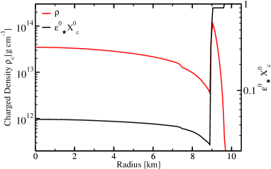
Figure 1: Radial profiles of the density of the charged component and of the factor $\varepsilon^{0}_{\star}X^{0}_{c}$ for our fiducial stellar model with a radius $R=12.26\,$km ($r=10.08\,$km) and a mass $M=1.4\mathrm{M}_{\odot}$. Note that in this plot and throughout the paper we use the coordinate radius $r=\Phi^{2}R$.

2.4 Magnetic field strength

The definition of the magnetic field strength varies in the literature between different authors. Colaiuda & Kokkotas (2011) and van Hoven & Levin (2012) used the polar magnetic field strength, Passamonti & Lander (2013) took the average magnetic field in the stellar volume, while observational astronomers usually refer to the equivalent magnetic field of a rotating uniformly magnetised sphere (see e.g. Olausen & Kaspi, 2013). In our previous work we have not been consistent in that respect either: in Gabler et al. (2011, 2012) we used the magnetic field strength at the pole. In Gabler et al. (2013b) we also refer to the polar value and, to better compare with the spin-down estimate, we used in addition an equivalent magnetic field strength of a uniformly magnetised sphere that would cause the same spin-down as in our model. In Gabler et al. (2013a) we take the average surface magnetic field strength as reference.

Ultimately, we want to compare our magnetic field estimates directly to those of the spin-down estimates. Therefore, similarly to Gabler et al. (2013b) we use here the magnetic field strength of a uniformly magnetised sphere that has the same magnetic dipole moment as the corresponding model, i.e. both our model and the sphere would have the same spin-down. However, in Gabler et al. (2013b), we did not rescale the magnetic field strength to a sample model of a neutron star with a radius $R=10\,$km, which we will do here. The equivalent magnetic field strength is thus

$$\bar{B}=\frac{m}{(10\,\mathrm{km})^{3}}\left(\frac{10\,\mathrm{km}}{R}\right)^{2}\,,$$ (19)

where $m$ is the magnetic dipole moment of the equilibrium configuration and the second factor corrects for the moment of inertia in the spin-down formula. For our fiducial model ($R=12.26\,$km, $M=1.4\mathrm{M}_{\odot}$) the equivalent magnetic field strength is roughly half of the field strength at the polar axis $\bar{B}\sim 0.56B_{\mathrm{pole}}$.

3 Low frequency oscillations with realistic entrainment

We study the superfluid magneto-elastic oscillations of our background magnetar model which is calculated with the RNS code. It has a mass $M=1.4\mathrm{M}_{\odot}$ and a radius $R=12.26\,$km. As described in the previous section, we take into account a realistic EoS (APR+DH) including the stratification resulting from a variable proton fraction in the core and the structure of the solid crust. We further consider the entrainment between protons and neutrons, which strictly speaking should vanish in models with non-superconducting protons. In this section we describe the features of the oscillations caused by the presence of superfluid neutrons and we study their behaviour at different magnetic field strengths. The resolution for the numerical simulations is $150\times 80$ zones for $r\times\theta=[0\,\text{km},10\,\text{km}]\times[0,\pi]$.

3.1 Classification of different magneto-elastic oscillations

Oscillation	specification	continuum (C)	Gabler et al.	Colaiuda et al.	Passamonti	vanHoven &	this work
type		or discrete (D)	Cerdá-Durán et al.	Sotani et al.	et al.	Levin
Alfvén/magneto-elastic	upper	C	$U^{(\pm)}_{n}$	$U^{\mathrm{odd/even}}_{n}$	$U^{(\pm)}_{n}$	turning point	$U_{n}^{\mathrm{surf}}$ , $U_{n}^{\mathrm{core}}$
Alfvén/magneto-elastic	edge	C	$E^{(\pm)}_{n}$	$L^{\mathrm{odd/even}}_{n}$	$L^{(\pm)}_{n}$	edge	$E_{n}$
Alfvén	lower	C	$L^{(\pm)}_{n}$	$C_{n}$	$C_{n}$	turning point	$L_{n}$
shear mode		D	crustal	crustal	${}^{l}t_{n}$	crustal	${}^{l}t_{n}$
discrete magneto-elastic		D	-	discrete Alfvén	${}^{l}t_{n}^{\ast}$	elasto-magnetic	${}^{l}U_{n}$

Table 1: Comparison of the notation used by different groups for the classification of oscillations. Here (last column), we continue employing the notation of Upper (U), Edge (E), and Lower (L) oscillations as in our previous work (Cerdá-Durán et al., 2008; Gabler et al., 2012, 2013b, 2013a). However, we will omit the symmetry label $(\pm)$ and introduce some additional specifications. (See main text for details.)

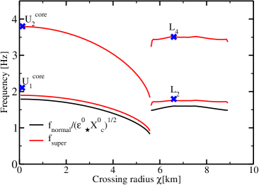
Figure 2: Semi-analytic, low-frequency spectrum of several continuum magneto-elastic oscillations for our magnetar model at $\bar{B}=5\times 10^{13}\,$G. The red lines include superfluid effects, while the black lines and correspond to the rescaled spectrum without superfluidity. The corresponding oscillation frequencies obtained in the simulations including superfluidity are indicated by blue crosses (compare also with Fig. 3).

As we discuss below, new structures in the QPO families appear in our model as a consequence of the inclusion of superfluidity. Therefore, to accommodate for the new oscillations we need to improve the notation employed for the classification of the oscillations, both compared to other work and to our previous work (Gabler et al., 2012, 2013b, 2013a). In these references we classified the oscillations according to their location within the Alfvén continuum (see also Table 1):

• Upper QPOs that are related to the upper turning point of the spectrum, close to the polar axis.

• Edge QPOs that are located at the edge of the spectrum close to the region of closed field lines near the equatorial plane.

• Lower QPOs that appear in the closed field line region.

As an example, we plot in Fig. 2 a spectrum for our model with $\bar{B}=5\times 10^{13}\,$G as a function of the radius $\chi$ at which the corresponding field line crosses the equatorial plane. The spectrum is obtained with our semi-analytic model (Cerdá-Durán et al., 2008; Gabler et al., 2012) which is based on the integration of the Alfvén speed along a given magnetic field line and by assuming perfect reflection of the oscillations at the core-crust interface. In this example, the Upper QPOs are located at $\chi=0$ km, the Edge QPOs at $\chi\sim 5.5\,$km and the Lower QPOs at $\chi\sim 6.5\,$km (confined to the region of magnetic field lines that close inside the core, $6\,{\rm km}<\chi<9\,$km). The larger deviation for $U_{1}^{\mathrm{core}}$ is expected, because of the limited accuracy of the semi-analytic model for long wavelengths (Cerdá-Durán et al., 2008).

Figure 3: Amplitude and phase distributions (resulting from the Fourier transform of the velocity evolution) for the strongest QPOs with frequencies up to $\sim 10\,$Hz, for $\bar{B}=5\times 10^{13}\,$G . Top row: Amplitude distribution. The colour scale ranges from white-blue (minimum) to red-black (maximum). Bottom row: Phase distribution. The colour scale ranges from blue ($\theta=-\pi/2$) to orange-red ($\theta=\pi/2$). The crust is indicated by the region between the dashed black lines and magnetic field lines are plotted in magenta. Notice that the plots for the ${\rm L}_{2}$ and ${\rm L}_{4}$ oscillations contain residual amplitudes outside the region of closed magnetic field lines, due to other, nearby QPOs. Also, sudden jumps from red to blue colour in the phase distribution are no discontinuities, but are caused by the phase crossing multiples of $\pi$ (the phase changes continuously throughout the star by several such multiples).

To allow for a unique identification of the members of each of the QPO classes U, E, and L we had previously introduced a superscript + (-) for QPOs that are symmetric (antisymmetric) with respect to the equatorial plane, and a subscript $n\in\{0,1,2,\dots\},$ which indicated the fundamental $(n=0)$ oscillation and the respective overtones $(n\geq 1)$. For example, the members of the class of symmetric upper QPOs were denoted as $U^{+}_{0}$, $U^{+}_{1}$, $U^{+}_{2}$, $\dots$ . To better discriminate the different QPOs, we introduce here additional specifications, such as $U_{n}^{\mathrm{core}}$ and $U_{n}^{\mathrm{surf}}$ to indicate oscillations $U$ that are confined to the core or reach the surface, respectively. Moreover, in this work $n$ gives the number of maxima along the field lines, but not the overtone in a particular family. This notation is unique for oscillations that are symmetric or antisymmetric with respect to the equatorial plane, and therefore we will omit the explicit indication of symmetry $(\pm)$ from now on. An even $n$ directly implies antisymmetry, while an odd $n$ implies symmetry. We also introduce discrete magneto-elastic oscillations ${}^{l}U_{n}$ in analogy to pure crustal shear modes ${}^{l}t_{n}$. For the latter, $l$ is the spherical harmonic index in the $\theta$-direction and $n$ is the number of maxima in the radial direction. Correspondingly, for the discrete magneto-elastic oscillations, we use $l$ as the number of maxima inside the crust across magnetic field lines and $n$ as the number of maxima throughout the star along the magnetic field lines in the region where the oscillation dominates.

3.2 General description of the oscillations

In models without superfluidity, the observed low-frequency QPOs were explained as magneto-elastic oscillations (Gabler et al., 2011, 2012, 2013b). For very weak magnetic fields of $\bar{B}\lesssim 10^{13}\,$G, torsional shear oscillations were obtained, which could explain some of the observed QPO frequencies. However, these oscillations were efficiently damped into the core for magnetic fields strengths in the range $10^{13}\lesssim\bar{B}\lesssim 10^{15}\,$G. In this case, Alfvén oscillations in the core were reflected at the core-crust interface and the oscillations were confined to the core. At $\bar{B}\gtrsim 10^{15}\,$G, the oscillations could penetrate into the crust and reach the surface. For both magnetic field regimes the oscillations had similar structures with one up to several maxima along the magnetic field lines and no particular structure perpendicular to the field lines (see e.g. figure 10 in Gabler et al., 2012).

Including superfluid effects, we find that the behaviour of the oscillations at low magnetic field strengths ($\bar{B}<10^{14}\,$G) is very similar to non-superfluid models. The structure of the dominant oscillations is shown in Fig. 3 for $\bar{B}=5\times 10^{13}\,$G, which also shows the magnetic field lines in magenta colour. The main difference superfluidity brings is that the oscillation frequencies are scaled upwards roughly by the average of $\varepsilon^{0}_{\star}X^{0}_{c}$ along the corresponding magnetic field line. In the top row of Fig. 3 we plot the magnitude of the complex Fourier amplitudes of the velocity of the perturbation for each point of our numerical grid at the frequencies of the first five Upper oscillations, $U_{1}^{\mathrm{core}}$ to $U_{5}^{\mathrm{core}}$, which are confined to the core, and the two Lower oscillations $L_{2}$ and $L_{4}$. The colour scale spans from white-blue (minimum) to red-black (maximum). In the bottom row of Fig. 3 we show the corresponding phase obtained from the Fourier analysis. Here, the colour scale spans from $-\pi/2$ (blue) to $+\pi/2$ (orange-red). Jumps from red to blue are no discontinuities, but are caused by the phase crossing multiples of $\pi$. For example, in the region of open field lines, the phase changes continuously throughout the star by several such multiples, i.e. $\phi=\phi_{0}+N\pi$, where $N$=1, 2, …. and $\phi_{0}$ is the phase at along the axis. More specifically, for $U_{2}^{\mathrm{core}}$ (second column in Fig. 3) the phase changes from green ($\phi=\phi_{0}$) to red/blue ($\phi=\phi_{0}+\pi/2$), again to green ($\phi=\phi_{0}+\pi$) and to red ($\phi=\phi_{0}+3\pi/2)$, etc. In the region of open field lines a total phase change of roughly $\Delta\phi\sim 7\pi/2$ can be observed for this oscillation. Similarly, all Upper oscillations $U_{n}^{\mathrm{core}}$ show a continuous change of phase in the region of open field lines, which underlines their characterization as continuum oscillations, rather than being discrete modes. Notice that in the region of open field lines confined to the core, the phase does not change along individual magnetic field lines. In contrast, the $L_{2}$ and $L_{4}$ oscillations in the region of closed field lines, show a varying phase along the field lines.(The resolution in these simulations was not sufficient to clearly show the phase changes for some oscillations).

All of the properties of the oscillations described in the previous paragraph are also present in non-superfluid models. The frequencies obtained for the $U_{n}^{\mathrm{core}}$ and $L_{n}$ oscillations agree very well with our semi-analytic model, see Fig. 2. When including superfluid effects, major differences arise for magnetic fields stronger than $10^{14}\,$G. Firstly, the lowest magnetic field strength at which the oscillations can reach the surface is reduced significantly to $\bar{B}\gtrsim{\rm few}\times 10^{14}\,$G compared to $\bar{B}\gtrsim 10^{15}\,$G in the normal fluid case (Gabler et al., 2012). Similarly, van Hoven & Levin (2011) found a strong damping of crustal motion for magnetic field strengths $\bar{B}<10^{15}\,$G, if the core neutrons are normal. Secondly, the oscillations now have structures also perpendicular to the magnetic field lines.

Figure 4: Radial profiles of the propagation speeds of magneto-elastic oscillations for different magnetic field strengths, close to the polar axis. Solid lines correspond to superfluid neutrons and dashed lines to normal matter. The crust starts at $\sim 9\,$km, and the brown dashed lines indicates the Alfvén velocity in the crust.

The penetration of oscillations into the crust region depends on the impedance mismatch between crust and core. To some extend this is related to the relative amplitude of the Alfvén velocity compared to that of the shear velocity in the crust (see Gabler et al., 2012; Link, 2014, for a more detailed discussion). In Fig. 4 we plot the different propagation velocities near the polar axis for different magnetic field strengths and for simulations with (solid lines) and without (dashed lines) superfluid neutrons. For very low magnetic fields, $\bar{B}\lesssim 10^{14}\,$G, the Alfvén velocity in the core is much smaller than the shear velocity at the base of the crust and the impedance mismatch is large. In this case, most incoming waves are reflected at the core-crust interface. The interface acts like a solid wall, where the waves get reflected back into the interior. The reflected oscillations stay confined to the core and have a node at the core-crust interface (see top row of Fig. 3). With increasing magnetic field strength the difference in propagation velocity and impedance decreases and not all of the waves are reflected. Therefore, the oscillations start to have non-negligible amplitudes in the crust.

Fig. 4 also shows that in the superfluid case the Alfvén velocity is higher than in the normal fluid case for a given magnetic field strength. Hence, the propagation velocities at both sides of the crust-core interface differ less and also the impedance mismatch is smaller. These smaller differences allow the oscillations to reach the surface at lower magnetic field strengths if neutrons are superfluid. For example, at $5\times 10^{14}\,$G the Alfvén velocity in the core equals the propagation speed in the crust (solid red line in Fig. 4), and there should be weak reflection for the considered field line compared to weaker magnetic fields.

Our simulations exhibit the expected behaviour, as can be seen in Figs. 3 and 5. At $\bar{B}=5\times 10^{13}\,$G (Fig. 3), all oscillations are confined to the core, while at $\bar{B}=5\times 10^{14}\,$G (Fig. 5) oscillations like ${}^{2}U_{2}$, ${}^{2}U_{4}$, and ${}^{3}U_{5}$, display a strong magneto-elastic character right up to the surface. At this magnetic field strength, other oscillations (such as $U_{2}^{\mathrm{core}}$, $U_{3}^{\mathrm{core}}$, $U_{4}^{\mathrm{core}}$) show only a partial excitation in the crust with an amplitude distribution that is similar to that of shear oscillations. This is due to partial reflection of magnetic field lines which are far from the pole, since i) there is still a mismatch of the impedances at the core-crust interface , and ii) the angle changes under which the magnetic field enters into the crust.

In addition to the different behaviour regarding the reflection at the core-crust interface, the structure and the properties of the oscillations also change when including superfluid effects. To discuss this, we will use Figs. 5 and 6 which show the results of the Fourier transform at the frequencies of the dominant oscillations for $\bar{B}=5\times 10^{14}\,$G and $\bar{B}=2\times 10^{15}\,$G, respectively. The simulation time was $1.350\,$s and $0.338\,$s, respectively which corresponds to about 80 oscillation periods of the lowest frequency oscillation. As in Fig. 3, the top row in both panels show the Fourier amplitude and the bottom row the corresponding phase, and we employ the same colour scale. At $5\times 10^{14}\,$G (Fig. 5), there are two distinct groups of oscillations, one that consists of oscillations showing an Alfvén character confined to the core and a very weak shear-oscillation character in the crust (such as $U_{2}^{\mathrm{core}}$ to $U_{6}^{\mathrm{core}}$), and the other displaying a strong magneto-elastic character up to the surface (${}^{1}U_{3},^{2}U_{2},^{2}U_{4},^{3}U_{5},^{6}U_{6})$.

In addition, the two groups have different phase properties. The phase of oscillations belonging to the first group, is continuous in the region of their largest amplitudes. For the second group with the strong magneto-elastic character up to the surface, the phase is very nearly constant $(^{2}U_{2},^{2}U_{4},^{6}U_{6})$ or only shows a small variation $(^{1}U_{3},^{3}U_{5})$. It is important to note that at nodal lines, the computation of the phase has large numerical errors and the constancy of the phase should only be judged by its value in regions for from nodal lines.

However, there are some oscillations like ${}^{3}U_{7},^{4}U_{6},$ and ${}^{5}U_{7}$, that seem not to match clearly into one or the other group. They have intermediate amplitudes inside the crust, and their phase varies in different parts of the neutron star. For ${}^{3}U_{7}$, which has its maximal amplitudes between the 6th and 7th plotted field line (magenta lines) the phase in this area and the part of the crust near by the equatorial plane is almost constant. Only close to the polar axis, where an overlap with a ${}^{?}U_{5}$ oscillation appears, the phase varies modestly. Oscillations ${}^{4}U_{6}$ and ${}^{5}U_{7}$ show a nearly constant phase in their dominant regions close to the polar axis and inside the crust. Notice that for these two oscillations there is an overlap with edge modes excited at the last open field line, which have a different phase and a different number of nodal lines than the dominant part of the oscillation. In all these three cases the phase of the oscillation actually helps to identify the dominating oscillation by indicating which parts of the neutron star oscillate together and have the same phase. Problems for a clear identification of the oscillations are small amplitudes compared to the dominant oscillations and limited resolution for oscillations with increasing $l$ and $n$. Additionally, a high $n$ and low $l$ oscillation may have a very similar frequency compared to a low $n$ but high $l$. Then both oscillations may appear in the same plot of a Fourier amplitude complicating a clear characterization (see e.g. ${}^{3}U_{7}$ and ${}^{?}U_{5}$ in Fig. 5).

Figure 5: Discrete Fourier transform of the velocity of the strongest QPOs at $\bar{B}=5\times 10^{14}\,$G with frequencies up to $\sim 100\,$Hz. First and third row: Fourier amplitude. Second and fourth row: Corresponding phases. Colour scales as before in Fig. 3.

For stronger magnetic fields, $\bar{B}\sim 2\times 10^{15}\,$G, the picture changes drastically and we only find coherent oscillations that reach the up to the surface. In the corresponding Fig. 6, we also see that the oscillations show structure perpendicular to the field lines. In contrast, for non-superfluid models (Gabler et al., 2012) the oscillations have a simpler structure with only one maximum perpendicular to the field lines. A similar situation appears in the superfluid case when considering a weaker magnetic field, $\bar{B}\sim 5\times 10^{13}\,G$; compare Fig. 3 in this work with Fig. 10 in Gabler et al. (2012). For the even stronger magnetic fields analysed, $\bar{B}>5\times 10^{15}\,G$, the oscillations become again dominated by the magnetic continuum, they have continuous phases and a simple structure with only one maximum perpendicular to the magnetic field lines. In fact, they look very similar to the oscillations in Fig. 3 that are located near the polar axis. However, for stronger magnetic fields they exhibit a maximum at the surface analogous to normal fluid models.

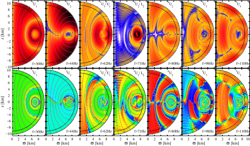
Figure 6: Discrete Fourier transform of the velocity of the strongest QPOs at $\bar{B}=2\times 10^{15}\,$G with frequencies up to $\sim 200\,$Hz. First and third row: Fourier amplitude. Second and fourth row: Corresponding phases. Colour scales as before in Figs. 3 and 5.

3.3 Coherent oscillations

We turn now to discuss coherent oscillations with constant phase. They only exist above a critical magnetic field strength, reach the magnetar surface and have much higher amplitudes than those of the continuum oscillations of the core. Inside the crust, the coherent oscillations look somewhat similar to pure crustal modes. For example, ${}^{2}U_{2}$ and ${}^{2}U_{4}$ resemble ${}^{2}t_{0}$, or ${}^{3}U_{5}$ resembles ${}^{3}t_{0}$ (cf. Fig. 5). Similar oscillations have been reported by van Hoven & Levin (2011, 2012), who found shear modes that seemed to be shifted into the gap of the continuum of the core if the crust was fixed. Discrete (Alfvén) modes were found in the simulations of Colaiuda & Kokkotas (2011) in models without superfluid effects. These modes were also (partially) interpreted as crustal modes that exist in the gap of the continuum of the core.

The coherent oscillations with constant phase found here may be related to these ‘gap modes’, although we interpret them in a different way. They should not be mistaken for shifted pure crustal shear modes for the following reasons: (i) Their frequencies do not match the shear mode frequencies of the crust, which are given in Table 2. For example at $\bar{B}=5\times 10^{14}\,$G the frequencies of the coherent oscillations are $f_{{}^{2}U_{2}}=22\,$Hz, $f_{{}^{2}U_{4}}=40\,$Hz and $f_{{}^{2}t_{0}}=26.5\,$Hz, or $f_{{}^{3}U_{5}}=58\,$Hz and $f_{{}^{3}t_{0}}=41.9\,$Hz. (ii) Different coherentoscillations have similar structure within the crust, e.g. ${}^{2}U_{2}$ and ${}^{2}U_{4}$ at $\bar{B}=5\times 10^{14}\,$G look very similar to ${}^{2}t_{0}$ (inside the crust). (iii) When increasing the magnetic field strength further, the structure of the oscillations inside the crust can deviate significantly from the structure of crustal modes. A good example is provided by the oscillations ${}^{2}U_{4}$,${}^{4}U_{4}$ and ${}^{6}U_{4}$ at $\bar{B}=2\times 10^{15}\,$G shown in Fig. 6.

$n$	0	0	0	0	0	1
$l$	2	3	4	5	6	2
${}^{l}f_{n}$	26.5	41.9	56.2	70.1	93.8	782.6

Table 2: Frequencies (in Hz) of the crustal shear modes of our fiducial model.

We interpret our simulations as follows. For weak magnetic fields, $\bar{B}\lesssim\mathrm{few}\,10^{14}\,$G, the oscillations are confined to the core, crustal modes are damped efficiently, and the dominant oscillations are Alfvén oscillations of the continuum. For stronger fields, a few $10^{14}\,\mathrm{G}\lesssim\bar{B}\lesssim\mathrm{several}\,10^{15}\,$G, the difference of the corresponding propagation velocities at the core and the crust is small (Fig. 4). Thus, the coupling of the crust to the Alfvén oscillations of the core is very efficient. Additionally, for such values of $\bar{B}$, the oscillations can enter into the crust where they are still dominated by the shear modulus. This leads to a strong interaction of oscillations of different field lines. This coupling is weaker in normal fluid models because, as mentioned before, the oscillations are reflected at the core-crust interface for significantly stronger magnetic fields than for superfluid models. Therefore, once they enter into the crust the oscillations are already of magneto-elastic type or dominated by the magnetic field inside the crust too. A strong coupling of continuum oscillations can lead to the formation of global modes, as Levin (2007) and Cerdá-Durán et al. (2008) showed for unphysically large dissipation and coupling through strong artificial viscosity, respectively. Normal modes are also found for highly tangled magnetic fields (Link & van Eysden, 2015; Sotani, 2015). Since we cannot show that the newfound oscillations show all properties of normal modes (like being orthogonal to each other and spanning a complete set), we call them constant phase oscillations (instead of discrete normal modes) to distinguish them from continuum oscillations. The new oscillations share properties of both, the Alfvén continuum oscillations (structures along the magnetic field lines extending into the core and frequency roughly scaling with $\bar{B}$, as we show below) and shear modes (structures orthogonal to field lines with constant phase). We thus conclude that the coherent oscillations are global magneto-elastic oscillations that are distinct from the purely shear modes of the crust.

One particular characteristic of the coherent oscillations is their splitting in the $\theta$-direction. The strong coupling caused by the crust allows for additional oscillation patterns of different angular dependencies (Figs. 5 or 6). This effect is reduced for very strong magnetic fields, i.e. $\bar{B}$ larger than several $10^{15}\,$G, when the magnetic field dominates over the shear modulus inside the crust, and the spectrum is formed by continuum oscillations. Without superfluidity, on the other hand, the oscillations are reflected at the core-crust interface $\bar{B}\lesssim 10^{15}\,$G, a value that is actually comparable to the shear modulus inside the crust. Therefore, for normal fluid cores, the range of magnetic field strengths in which coherent magneto-elastic oscillations can be observed is markedly narrowed down to about $10^{15}\,\mathrm{G}\lesssim\bar{B}\lesssim\mathrm{few}\times 10^{15}\,\mathrm{G}$. We note that in our previous work with normal fluid models we did not fine tune our simulations to span such a narrow range of values of $\bar{B}$, which explains the fact that the coherent oscillations went unnoticed in our examination.

It should be emphasized that the discovery of these new oscillations generates a difficult new conundrum. Namely, explaining how these constant phase oscillations could account for the observed QPOs in the giant flares of two magnetars estimated to have significantly different magnetic field strengths, $\bar{B}\sim 2.0\times 10^{15}\,$G for SGR 1806-20 and $\bar{B}\sim 7\times 10^{14}\,$G for SGR 1900+14, remains a challenging open issue.

3.4 Scaling of the oscillation frequencies with $\bar{B}$

Figs. 5 and 6 show that the oscillation frequencies depend on the magnetic field strength. In this Section, we investigate this dependence more systematically. To achieve this goal, we perform a new set of simulations with $\bar{B}=\{0.5,1,2.5,5,6,7,8,9,10,15,20,30\}\times 10^{14}\,$G using the same initial data, namely a perturbation with a mixed $l=2$ and $l=3$ angular dependence and a radial structure having zero amplitude both in the centre and at the core-crust interface, and reaching a maximum inside the core and at the surface of the magnetar. This initial perturbation should excite many different oscillations that represent the spectrum of the magnetar model.

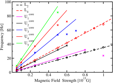
Figure 7: Frequencies of the continuum oscillations having the lowest frequencies at as a function of magnetic field strength. Symbols give the frequencies obtained from the simulations, and the lines are linear fits (see Table 3).

	$L_{2}$	$L_{4}$	$U_{1}^{\mathrm{core}}$	$U_{2}^{\mathrm{core}}$	$U_{3}^{\mathrm{core}}$	$U_{4}^{\mathrm{core}}$	$U_{5}^{\mathrm{core}}$
$b$ [Hz]	3.5	7.0	4.0	6.3	10.8	14.7	18.7

Table 3: Linear fits of the frequency $f\,[\mathrm{Hz}]=a+b\times\bar{B}[10^{14}\mathrm{G}]$ of the continuum oscillations of our superfluid model with realistic entrainment. For all Lower $L_{n}$ and Upper $U_{n}^{\mathrm{core}}$ oscillations that are confined to the core $a=0.0$.

We first study the continuum oscillations. Their frequencies are shown as a function of the magnetic field strength in Fig. 7. The symbols give the frequencies obtained with the Fourier transforms of the evolved data and the solid lines are the corresponding linear fits, whose parameters are given in Table 3. All Lower oscillations scale in the same way with the magnetic field strength such that $L_{n}=\frac{n}{2}L_{2}~{}~{}(n>2)$. For the Upper oscillations we find $U_{n}^{\mathrm{core}}=3.7n\,$Hz. The largest deviation from this scaling occurs for the two lowest QPOs, $U_{1}^{\mathrm{core}}$ and $U_{2}^{\mathrm{core}}$, as we already reported in Gabler et al. (2012). The frequencies of the higher overtones ($n>2$) are in near integer relations $\frac{f_{n}}{f_{m}}\sim\frac{n}{m}$. Fig. 7 also shows that with increasing magnetic field strength the frequencies of the calculated QPOs deviate significantly from our linear fits towards lower values. This is expected since, as we described in Gabler et al. (2012), the oscillations are no longer reflected efficiently from all parts of the core-crust interface as the field strength increases. Therefore, the oscillations move from the polar region towards the equatorial region, see e.g. the changing location of $U_{4}^{\mathrm{core}}$ in Figs. 3 and 5. Consequently, the corresponding frequencies in the continuum decrease. At magnetic field strengths $\bar{B}\gtrsim 8\times 10^{14}\,$G all Upper oscillations confined to the core disappear. They become coherent oscillations with constant phase, which can reach the surface.

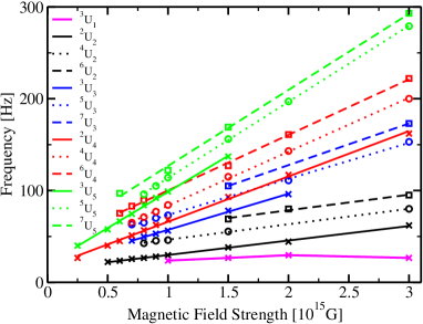
Figure 8: Frequencies of the coherent oscillations having the lowest frequencies at as a function of magnetic field strength. Symbols give the frequencies obtained from the simulations, and the lines are linear fits (see Table 4).

oscillation	${}^{2}U_{2}$	${}^{4}U_{2}$	${}^{6}U_{2}$	${}^{3}U_{3}$	${}^{5}U_{3}$	${}^{7}U_{3}$
$a$ [Hz]	14.0	29.6	44.5	17.8	34.2	37.0
$a_{l}^{\mathrm{fit}}$[Hz]	14.8	28.0	41.2	19.9	30.7	41.5
$b$ [Hz]	1.6	1.7	1.7	3.9	3.9	4.5
$b_{n}^{\mathrm{fit}}$ [Hz]	1.7	1.7	1.7	3.8	3.8	3.8

oscillation	${}^{2}U_{4}$	${}^{4}U_{4}$	${}^{6}U_{4}$	${}^{3}U_{5}$	${}^{5}U_{5}$	${}^{7}U_{5}$
$a$ [Hz]	16.7	24.7	39.5	19.9	30.6	43.8
$a_{l}^{\mathrm{fit}}$[Hz]	14.8	28.0	41.2	19.9	30.7	41.5
$b$ [Hz]	4.9	5.9	6.0	7.9	8.3	8.3
$b_{n}^{\mathrm{fit}}$[Hz]	5.9	5.9	5.9	8.0	8.0	8.0

Table 4: Linear fits of the frequency $f\,[\mathrm{Hz}]=a+b\times\bar{B}[10^{14}\mathrm{G}]$ of the coherent oscillations of our superfluid model with realistic entrainment. The approximate values of these parameters obtained by assuming $a=a_{l}^{\mathrm{fit}}$ and $b=b_{n}^{\mathrm{fit}}$ are also shown. See main text for details.

The coherent oscillations also scale directly with the magnetic field strength (see Fig. 8, and the corresponding linear fits in Table 4), which indicates that these oscillations cannot be crustal shear modes as the latter are independent of magnetic field strength. Furthermore, we see that oscillations having the same angular structure inside the crust, like ${}^{2}U_{2}$ and ${}^{2}U_{4}$, or ${}^{4}U_{2}$ and ${}^{4}U_{4}$, can have very different oscillation frequencies depending on the structure given by the number of nodes $n$ along the magnetic field lines. If these oscillations were crustal modes with no nodes in the radial direction inside the crust, they should have the same frequency only depending on $l$. The coherent oscillations also only appear for $\bar{B}\gtrsim 2.5\times 10^{14}\,$G, when the reflection of incoming oscillations at the core-crust boundary is no longer very strong. To fit the observed oscillations with a linear function $f=a+b\times\bar{B}[10^{14}\mathrm{G}]$, we also need to introduce an offset $a$. We prefer not to call the offset $a$ an asymptotic frequency for zero magnetic field strength, because for a vanishing magnetic field the coherent oscillations do not exist and only crustal modes survive. However, the presence of the offset $a$ also indicates that the coherent oscillations with constant phase are coupled, magneto-elastic oscillations that are not present without a solid crust. While the linear coefficient $b$ is nearly constant within one family of coherent oscillations with the same $n$, the offset $a$ increases with increasing $l$. For example, for $n=2$ and $l=\{2,3,4\}$ we find $a=\{14.0,29.6,44.5\}$Hz. We can fit the factor $b$ reasonably well to $b=b_{n}^{\mathrm{fit}}\sim(2.1n-2.457)\,$Hz. The offset $a$ for a given $l$ is also similar for different values of $n$, i.e. we can approximate $a=a_{l}^{\mathrm{fit}}=(1.6+6.6l)\,$Hz if $l$ is even, and $a=a_{l}^{\mathrm{fit}}=(3.7+5.4l)\,$Hz if $l$ is odd. Therefore, the complete fits read

$$f=\begin{cases}(1.6+6.6l+(2.1n-2.457)\bar{B}[10^{14}])\,\mathrm{Hz}&\text{$l$ even}\\ (3.7+5.4l+(2.1n-2.457)\bar{B}[10^{14}])\,\mathrm{Hz}&\text{$l$ odd}\end{cases}$$ (20)

With our assumptions that $a$ depends only on $l$, and $b$ depends only on $n$ we obtain reasonable fits to the measured values (Table 4). The oscillation frequencies scale with the number of nodes $n$ along the magnetic field lines, indicating the Alfvénic character of the oscillations. Pure Alfvén oscillations behave in the same way. The offset scales with the angular number, similar to pure crustal shear modes. This similarity is intuitive, because for very low magnetic field strength crustal modes should appear. To the accuracy of the simulations

$$a=a_{l}^{\mathrm{fit}}\sim\sqrt{(l-1)(l+2)},$$ (21)

as it is the case for the purely crustal shear modes. However, given the numerical accuracy of the results we cannot distinguish between Eq. (21) and the linear fit. Our fitting functions only allow us to understand the qualitative behaviour of the oscillations and not their actual behaviour since they are neither purely elastic nor purely magnetic.

3.5 Numerical viscosity and different damping due to phase mixing

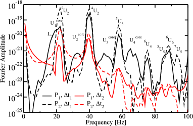
Figure 9: Fourier amplitude of the velocity at points $P_{1}$ ($\theta\sim 1.2\,$rad, $r\sim 3.5\,$km) in the core and $P_{2}$ ($\theta\sim 0.8\,$rad, $r\sim 9.2\,$km) in the crust. Black lines are the results for the time interval $\Delta t_{1}=[0\,\mathrm{ms},675\,\mathrm{ms}]$ and red lines for $\Delta t_{2}=[675\,\mathrm{ms},1350\,\mathrm{ms}]$.

At $\bar{B}=5\times 10^{14}\,$G we find coexisting continuum and coherent, constant phase oscillations. However, we expect the coherent oscillations to persist for longer times, because the continuum oscillations have a salient damping mechanism in the form of phase mixing.

In Fig. 9 we plot the Fourier amplitude of the velocity at two different locations inside the star, $P_{1}$ (in the core, $\theta\sim 1.2\,$rad, $r\sim 3.5\,$km) and $P_{2}$ (in the crust, $\theta\sim 0.8\,$rad, $r\sim 9.2\,$km), for different time intervals, $\Delta t_{1}=[0\,\mathrm{ms},675\,\mathrm{ms}]$ (black lines) and $\Delta t_{2}=[675\,\mathrm{ms},1350\,\mathrm{ms}]$ (red lines). In the first interval, a number of coherent oscillations (${}^{2}U_{2}$, ${}^{4}U_{2}$, ${}^{5}U_{3}$, ${}^{6}U_{4}$, ${}^{5}U_{5}$, ${}^{6}U_{6}$, and ${}^{7}U_{5}$) and continuum oscillations ($U_{1}^{\mathrm{core}}$, $U_{2}^{\mathrm{core}}$, $U_{3}^{\mathrm{core}}$, and $U_{4}^{\mathrm{core}}$) are excited initially. Both families are damped by the numerical dissipation of the code and, in addition, the continuum oscillations undergo phase mixing. These damping mechanisms lead to a reduced amplitude of the coherent oscillations during the second interval $\Delta t_{2}$, while the continuum oscillations disappear completely. The finer the spatial structure of the coherent oscillations, the faster the damping (Cerdá-Durán, 2010); as, for example, a comparison of the amplitudes of the oscillations ${}^{4}U_{2}$ and ${}^{5}U_{3}$ shows (Fig. 9). The coherent oscillations with highest frequencies and finest spatial structures (${}^{6}U_{4}$, ${}^{5}U_{5}$, ${}^{6}U_{6}$, and ${}^{7}U_{5}$) almost disappear completely due to numerical damping.

4 Parameter study of the entrainment effects

We turn next to investigate how the results change when considering different values for the mass fraction that participates in the Alfvén motion of the core. Purely nucleonic EoS, like the APR EoS we use, consider neutrons, protons, electrons, and muons. These EoS predict proton fractions of the order of $X_{c}\sim 0.1-0.2$ (Akmal et al., 1998) and effective masses that reduce this value to about $\varepsilon_{\star}X_{c}\sim 0.05$ (Chamel & Haensel, 2008). These values depend sensitively on the assumed composition in the neutron star core. For example, with the inclusion of hyperons (which are expected to appear from nuclear theory above a few times nuclear saturation density) the proton fraction may change to $X_{c}\sim 0.3$ (Baldo et al., 2000; Schulze & Rijken, 2011).

To investigate the effect on the oscillations of different compositions in the neutron star core, we vary the factor $\varepsilon_{\star}X_{c}$ throughout the core, rescaling it by a constant number to encode our ignorance about the true EoS properties of the core. In the following, the reported values of $\varepsilon_{\star}X_{c}$ will always refer to its central value $\varepsilon_{\star}X_{c}(r=0)$, e.g. our reference value given in the APR EoS is $\varepsilon_{\star}^{0}X^{0}_{c}(r=0)=0.0463$. For our analysis we perform a new set of simulations varying $\varepsilon_{\star}X_{c}$ from its value inferred from theoretical calculation of the EoS, $\varepsilon_{\star}X_{c}=\varepsilon^{0}_{\star}X^{0}_{c}$, to the upper limit given by the normal fluid model, $\varepsilon_{\star}X_{c}=1.0$. The magnetic field strengths considered are $\bar{B}=\{0.5,1,2.5,5,7.5,10,15,20\}\times 10^{14}\,$G, and the resolution employed is $150\times 80$ zones for $r\times\theta=[0\,\text{km},10\,\text{km}]\times[0,\pi]$.

From the propagation speeds (Eqs. (14) and (15)) we expect that the Alfvén velocity at a given $\bar{B}$ in the core scales like

$$v_{A}(\varepsilon_{\star}X_{c})\sim\frac{v_{A}(\varepsilon_{\star}X_{c}=1.0)}{\sqrt{\varepsilon_{\star}X_{c}}}\,.$$ (22)

Since the frequency of a pure Alfvén oscillation is proportional to the Alfvén speed, we expect the frequencies of the ‘core’ oscillations ($U_{1}^{\mathrm{core}},U_{2}^{\mathrm{core}},\cdots$) and Lower oscillations ($L_{2},L_{4},\cdots$) to scale like

$$f_{\mathrm{QPO}}\sim d_{0}\times\left(\varepsilon_{\star}X_{c}\right)^{d}\,,$$ (23)

with $d=-0.5$. This assumption roughly agrees with our semi-analytic model to calculate the spectra in Fig. 2. The spectrum of the non-superfluid model can be scaled roughly as that of the superfluid model by dividing it by $\sqrt{\varepsilon^{0}_{\star}X^{0}_{c}}$. Our simulations at $\bar{B}=5\times 10^{14}\,$G confirm this scaling approximately (see top two rows of Table 5). In particular, the Lower oscillations scale as expected with exponents $d=-0.50$ and $d=-0.51$. (See also the fits in Fig. 10.) For the ‘core’ oscillations the deviations are larger ($-0.59<d<-0.47$), which is probably related to the influence of the crust, where the reflection is not perfect. At $\bar{B}=5\times 10^{14}\,$G oscillations already enter partially into the crust, and coherent oscillations appear. In this regime, and for increasing magnetic field strength, the Upper oscillations move from the pole towards the equator, where the reflection at the core-crust interface is more efficient (Gabler et al., 2012). This spatial movement is accompanied by a shift in frequency, because the oscillation occurs at a different part of the continuum. This is visible in Fig. 2 where for increasing crossing radius $\chi$ the frequency of the continuum decreases. A similar behaviour is expected by changing $\varepsilon_{\star}X_{c}$ instead of the magnetic field strength. The Upper oscillations can enter into the crust more efficiently for low $\varepsilon_{\star}X_{c}$, thus their maxima are shifted towards the equator and their frequencies shift to lower values in the spectrum. For this reason, the frequency of the core oscillations measured in the simulations does not scale exactly as $d\sim-0.5$. For very weak magnetic fields, $\bar{B}\lesssim 5\times 10^{13}\,$G (where efficient reflection occurs and the Upper oscillations stay close to the polar axis) we thus expect a better agreement with $d=-0.5$. However, these are uninteresting magnetic field strengths for magnetars.

	$L_{2}$	$L_{4}$	$U_{1}^{\mathrm{core}}$	$U_{2}^{\mathrm{core}}$	$U_{3}^{\mathrm{core}}$	$U_{4}^{\mathrm{core}}$
$d_{0}$	3.76	7.33	4.23	7.62	10.99	10.74
$d$	-0.50	-0.51	-0.50	-0.47	-0.51	-0.59

	${}^{2}U_{2}$	${}^{4}U_{2}$	${}^{1}U_{3}$	${}^{3}U_{3}$	${}^{2}U_{4}$	${}^{4}U_{4}$	${}^{3}U_{5}$
$d_{0}$	16.2	16.7	23.3	35.1	40.4	50.9	55.0
$d$	-0.34	-0.58	-0.32	-0.33	-0.35	-0.34	-0.43

Table 5: Fittings of the frequencies $f\,[\mathrm{Hz}]=d_{0}\times\left(\varepsilon_{\star}X_{c}\right)^{d}$ of various oscillations for $\bar{B}=5\times 10^{14}\,$G (top) and $\bar{B}=2\times 10^{15}\,$G (bottom).

Figure 10: Scaling of the frequencies with the parameters $\varepsilon_{\star}X_{c}$ for the first few Upper and Lower oscillations that are confined to the core, for $\bar{B}=5\times 10^{14}\,$G. Lines are the fits with the parameters given in Table 5 and symbols are the results obtained in the simulations.

Regarding coherent oscillations (see the two bottom rows in Table 5 and Fig. 11), their scaling with the entrainment factor and the proton fraction, $\left(\varepsilon_{\star}X_{c}\right)^{d}$ (which varies between $d=-0.58$ and $d=-0.32$, with most oscillations scaling as $d\sim-1/3$) is not as close to $d=-0.5$ as for the continuum oscillations. Nevertheless, this weaker scaling is expected because coherent oscillations have non-vanishing amplitudes inside the crust where the fraction of charged component and the entrainment are not changed for different simulations. We note that for the oscillations ${}^{4}U_{2}$ and ${}^{3}U_{5}$, which were the hardest to identify, we actually failed to identify them for very low values of $\varepsilon_{\star}X_{c}(r=0)\lesssim 0.3$. This may explain the larger deviations ($d=-0.58$ and $d=-0.43$) respectively, from the $d\sim-1/3$ scaling of the rest of oscillations. Higher resolution and longer evolution times might reduce this discrepancy.

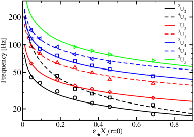
Figure 11: Scaling of the frequencies with the parameters $\varepsilon_{\star}X_{c}$ for the first few coherent oscillations ${}^{l}U_{n}$, for $\bar{B}=2\times 10^{15}\,$G. Lines are the fits with the parameters given in Table 5 and symbols are the results obtained in the simulations.

In the following, we proceed to find a general relation that describes the frequency of the dominant coherent oscillation ${}^{2}U_{2}$ for different magnetic field strengths and entrainment factors. The potential interest of deriving such an equation is that it may help constrain the state of the matter inside the core of the neutron star by simply estimating the factor $\varepsilon_{\star}X_{c}$, if the EoS, the stellar compactness, and the magnetic field strength are known. To derive this equation we make the following assumptions: (i) There is an offset $f^{0}_{{}^{2}U_{2}}$ which depends on $\varepsilon_{\star}X_{c}$, and may depend also on $l$ as we know from Eq. (20), but does not depend on $\bar{B}$; (ii) the frequency is approximately proportional to $\bar{B}$, as we have seen in Section 3.4; and (iii) the dependence on $\varepsilon_{\star}X_{c}$ can be described by a power law with exponent $b$. With these assumptions, we should find a relation of the form

$$f_{{}^{2}U_{2}}[\mathrm{Hz}]=f^{0}_{{}^{2}U_{2}}(\varepsilon_{\star}X_{c})+a_{{}^{2}U_{2}}\cdot\left(\varepsilon_{\star}X_{c}\right)^{b_{{}^{2}U_{2}}}\cdot\bar{B}\,.$$ (24)

The first information we need is $f^{0}_{{}^{2}U_{2}}$ as a function of $\varepsilon_{\star}X_{c}$, which we can obtain from the dependence of the frequency on the magnetic field strength according to

$$f\,[\mathrm{Hz}]=f^{0}_{{}^{2}U_{2}}(\varepsilon_{\star}X_{c})+a_{f^{0}}\times\bar{B}[10^{14}\mathrm{G}]\,.$$ (25)

Having found $f^{0}_{{}^{2}U_{2}}$ for different values of $\varepsilon_{\star}X_{c}$, we obtain a fitting function (see Table 6)

$\varepsilon_{\star}X_{c}~{}[\varepsilon^{0}_{\star}X^{0}_{c}]$	1	2	4	6	8	10	15
$\varepsilon_{\star}X_{c}[10^{-2}]$	4.6	9.2	18.5	27.8	37.0	46.3	69.5
$f^{0}_{{}^{2}U_{2}}\,$[Hz]	14.9	10.4	7.24	5.25	5.04	4.37	3.27
$a_{f^{0}}\,$[Hz]	1.47	1.41	1.19	1.06	0.90	0.84	0.71

Table 6: The frequency offset $f^{0}_{{}^{2}U_{2}}$ and the linear coefficient $a_{f^{0}}$ of the fitting functions Eq. (25) of different entrainment factors for the oscillation ${}^{2}U_{2}$.

$$f^{0}_{{}^{2}U_{2}}=f^{0}_{{}^{2}U_{2}}(\varepsilon_{\star}X_{c})=2.8\times(\varepsilon_{\star}X_{c})^{-0.55}\,\mathrm{Hz}\,.$$ (26)

Next, we determine the parameters $a_{{}^{2}U_{2}}$ and $b_{{}^{2}U_{2}}$ in Eq. (24) by simulating the oscillations for different $\varepsilon_{\star}X_{c}$ for three different magnetic field strengths, $\bar{B}=\{7.5,10,20\}\times 10^{14}\,$G. The resulting frequencies are fitted by the parameters given in Table 7 and the corresponding curves are plotted in Fig. 12.

Figure 12: Fitting functions defined in Eq. (24) (solid lines) for three different magnetic field strengths, $\bar{B}=\{7.5,10,20\}\times 10^{14}\,$G to obtain $f_{{}^{2}U_{2}}$ as a function of $\varepsilon_{\star}X_{c}$. Symbols give the frequencies obtained in the simulations.

$B[10^{14}G]$	$a_{{}^{2}U_{2}}$	$b_{{}^{2}U_{2}}$
7.5	0.65	-0.34
10	0.66	-0.34
20	0.67	-0.32
$\varnothing$	0.66	-0.33

Table 7: Parameters and their average for the fitting function $f\,[\mathrm{Hz}]=f^{0}_{{}^{2}U_{2}}(\varepsilon_{\star}X_{c})+a_{{}^{2}U_{2}}\cdot(\varepsilon_{\star}X_{c})^{b_{{}^{2}U_{2}}}\cdot\bar{B}[10^{14}\mathrm{G}]$ for the coherent oscillation ${}^{2}U_{2}$ for three magnetic field strengths.

The parameters obtained for different magnetic field strengths agree well with each other, i.e. we can use their averages (see Table 7) to finally obtain

$$f_{{}^{2}U_{2}}[\mathrm{Hz}]=2.8\times(\varepsilon_{\star}X_{c})^{-0.55}+0.66\left(\varepsilon_{\star}X_{c}\right)^{-0.33}\bar{B}[10^{14}\mathrm{G}]\,.$$ (27)

Fig.12 shows that the frequencies for the lowest values of $\varepsilon_{\star}X_{c}$ deviate most significantly from the fit (Eq. (27)). For such low values the crust, where the entrainment and the fraction of charged particles is constant, sets a minimal timescale needed by the oscillations to cross the crust. This shortest travel time corresponds to the maximum frequency of the oscillations. As an extreme example, one could increase the propagation speed of the oscillation in the core to infinity by setting $\varepsilon_{\star}X_{c}=0$. However, in this case the maximum frequency is set by the crust alone (and is finite).

A final remark about Eq. (27) is in order: coherent oscillations with constant phase exist not for all possible combinations of magnetic field strengths and choices of $\varepsilon_{\star}X_{c}$. For very high $\bar{B}$, Alfvén oscillations reach the surface of the magnetar while for very weak magnetic fields the oscillations are confined to the core. Likewise, the range of magnetic field strengths in which coherent oscillations can occur is wider for lower values of $\varepsilon_{\star}X_{c}$ and fairly narrow for non-superfluid matter $\varepsilon_{\star}X_{c}=1.0$ (Gabler et al., 2013a).

5 Conclusions

We have studied the effects of superfluidity on the magneto-elastic oscillations of magnetars for a realistic equation of state including stratification and entrainment. Our results confirm those of previous studies (Gabler et al., 2013a; Passamonti & Lander, 2014) which showed the existence of both, continuous phase and coherent, constant phase oscillations in the spectra of magnetars. In particular, we showed that for typical magnetar field strengths ($\bar{B}\lesssim 5\times 10^{15}\,$G) the continuous phase oscillations, also found in normal fluid models, are confined to the core of the neutron star, i.e. they are Alfvén oscillations that are reflected at the core-crust interface and have negligible amplitudes inside the crust (see Fig. 3).

Coherent oscillations, with properties very different from continuous phase oscillations, are a consequence of the relatively stronger coupling of oscillations through the crust in superfluid models compared to their normal fluid counterparts. Our simulations have shown that coherent oscillations have the following properties: (i) They have non-vanishing amplitudes inside the crust (see Figs. 5 and 6). (ii) They appear (depending on the proton fraction and the entrainment) at $\bar{B}\gtrsim\mathrm{few}\times 10^{14}\,G$ (see Fig. 8). (iii) The increased coupling of different field lines through the crust allows these oscillations to have structures perpendicular to the field lines. As a result, an oscillation, which is characterised by the number of maxima $n$ along field lines only, splits now into several oscillations with different numbers of maxima $l$ perpendicular to the field lines (see Figs. 5 and 6). (iv) Due to the constant phase, the newly found oscillations are longer-lived (see Fig. 9). (v) Their frequencies scale linearly with the magnetic field strength, but have a constant offset. They are thus clearly neither pure Alfvén oscillation nor crustal shear modes. These ${}^{l}U_{n}$ oscillations are the most promising candidates for explaining the observed low frequency, $f\lesssim 155\,$Hz, QPOs in magnetars.

We use the term coherent oscillations instead of discrete normal modes, because the latter would imply that the oscillations are orthogonal and form a complete set of eigenmodes, which we cannot proof rigorously with our direct numerical simulations. Performing a normal mode analysis it may be possible to show that discrete normal modes indeed exist. Sotani (2015) found normal modes in magnetar models with highly tangled magnetic fields. However, these eigenmodes are different from our coherent oscillations with constant phase, because they do not have a frequency offset of the order of the crustal shear modes and they do exist at all magnetic field strengths, i.e. there is no continuum in the limit of weak or strong magnetic fields. However, the strong coupling due to the high entanglement may play a similar role as the strong coupling of different field lines through the crust in this work.

In our study, the effects of changing the composition and entrainment were encoded into a single parameter, $\varepsilon_{\star}X_{c}$. As expected, the frequencies of the oscillations confined to the core, $U^{\mathrm{core}}_{n}$ and $L_{n}$, scale like $f\sim d_{0}\sqrt{\varepsilon_{\star}X_{c}}$. Coherent oscillations, on the contrary, have a different scaling, $f\sim f^{0}(\varepsilon_{\star}X_{c})+a_{f^{0}}\left(\varepsilon_{\star}X_{c}\right)^{-1/3}\bar{B}$, where the exponent is $-1/3$ for several ${}^{l}U_{n}$ oscillations for a given magnetic field strength. In the particular case of ${}^{2}U_{2}$, it was obtained for three different magnetic field strengths.

The superfluid magneto-elastic oscillations discussed in this work (see also Gabler et al. (2013a); Passamonti & Lander (2014)) allow to explain qualitatively, and simultaneously, both the low- and high-frequency QPOs observed in magnetars. However, our model still has to be improved. On the one hand, it does not include the possibility of superconducting protons (which may be destroyed due to the ultra-strong magnetic fields present in magnetars). On the other hand, we do neither consider a highly tangled magnetic field nor mixed toroidal and poloidal magnetic fields that may change the spectrum (Colaiuda & Kokkotas, 2012; Sotani, 2015). We plan to account for these two main missing ingredients in the near future and address these issues in further work. Another important open question is how the oscillations of a neutron star may modulate its X-ray emission. To understand the modulation mechanism it would be necessary to estimate the amplitude of the oscillations and to be able to compare them with the properties of observed QPOs. Needless to say, to really advance in our understanding of QPOs, we eagerly need to increase the available observational data. There is still no unambiguous pattern in the frequency spacing of the QPOs. Recent work aimed at detecting QPOs in normal magnetar bursts appears very promising (Huppenkothen et al., 2014a; Huppenkothen et al., 2014c) and we strongly encourage further studies in this direction.

References

- Akmal et al. (1998) Akmal A., Pandharipande V. R., Ravenhall D. G., 1998, Phys. Rev. C, 58, 1804
- Anderson & Itoh (1975) Anderson P. W., Itoh N., 1975, Nature, 256, 25
- Andersson et al. (2002) Andersson N., Comer G. L., Langlois D., 2002, Phys. Rev. D, 66, 104002
- Andersson et al. (2004) Andersson N., Comer G. L., Grosart K., 2004, MNRAS, 355, 918
- Andersson et al. (2009) Andersson N., Glampedakis K., Samuelsson L., 2009, MNRAS, 396, 894
- Baldo et al. (2000) Baldo M., Burgio G. F., Schulze H.-J., 2000, Phys. Rev. C, 61, 055801
- Baym et al. (1969) Baym G., Pethick C., Pines D., 1969, Nature, 224, 673
- Bocquet et al. (1995) Bocquet M., Bonazzola S., Gourgoulhon E., Novak J., 1995, A&A, 301, 757
- Cerdá-Durán (2010) Cerdá-Durán P., 2010, Classical and Quantum Gravity, 27, 205012
- Cerdá-Durán et al. (2008) Cerdá-Durán P., Font J. A., Antón L., Müller E., 2008, A&A, 492, 937
- Cerdá-Durán et al. (2009) Cerdá-Durán P., Stergioulas N., Font J. A., 2009, MNRAS, 397, 1607
- Chamel (2008) Chamel N., 2008, MNRAS, 388, 737
- Chamel (2012) Chamel N., 2012, Phys. Rev. C, 85, 035801
- Chamel & Haensel (2008) Chamel N., Haensel P., 2008, Living Reviews in Relativity, 11
- Colaiuda & Kokkotas (2011) Colaiuda A., Kokkotas K. D., 2011, MNRAS, 414, 3014
- Colaiuda & Kokkotas (2012) Colaiuda A., Kokkotas K. D., 2012, MNRAS, 423, 811
- Colaiuda et al. (2009) Colaiuda A., Beyer H., Kokkotas K. D., 2009, MNRAS, 396, 1441
- Deibel et al. (2014) Deibel A. T., Steiner A. W., Brown E. F., 2014, Phys. Rev. C, 90, 025802
- Douchin & Haensel (2001) Douchin F., Haensel P., 2001, A&A, 380, 151
- Duncan (1998) Duncan R. C., 1998, ApJ, 498, L45
- Duncan & Thompson (1992) Duncan R. C., Thompson C., 1992, ApJ, 392, L9
- Gabler et al. (2011) Gabler M., Cerdá Durán P., Font J. A., Müller E., Stergioulas N., 2011, MNRAS, 410, L37
- Gabler et al. (2012) Gabler M., Cerdá-Durán P., Stergioulas N., Font J. A., Müller E., 2012, MNRAS, 421, 2054
- Gabler et al. (2013a) Gabler M., Cerdá-Durán P., Stergioulas N., Font J. A., Müller E., 2013a, Physical Review Letters, 111, 211102
- Gabler et al. (2013b) Gabler M., Cerdá-Durán P., Font J. A., Müller E., Stergioulas N., 2013b, MNRAS, 430, 1811
- Gabler et al. (2014) Gabler M., Cerdá-Durán P., Stergioulas N., Font J. A., Müller E., 2014, MNRAS, 443, 1416
- Gearheart et al. (2011) Gearheart M., Newton W. G., Hooker J., Li B.-A., 2011, MNRAS, 418, 2343
- Glampedakis & Jones (2014) Glampedakis K., Jones D. I., 2014, MNRAS, 439, 1522
- Glampedakis et al. (2006) Glampedakis K., Samuelsson L., Andersson N., 2006, MNRAS, 371, L74
- Glampedakis et al. (2011) Glampedakis K., Andersson N., Samuelsson L., 2011, MNRAS, 410, 805
- Graber et al. (2015) Graber V., Andersson N., Glampedakis K., Lander S. K., 2015, MNRAS, 453, 671
- Gusakov & Haensel (2005) Gusakov M. E., Haensel P., 2005, Nuclear Physics A, 761, 333
- Hambaryan et al. (2011) Hambaryan V., Neuhäuser R., Kokkotas K. D., 2011, A&A, 528, A45+
- Huppenkothen et al. (2014a) Huppenkothen D., et al., 2014a, ApJ, 787, 128
- Huppenkothen et al. (2014b) Huppenkothen D., Watts A. L., Levin Y., 2014b, ApJ, 793, 129
- Huppenkothen et al. (2014c) Huppenkothen D., Heil L. M., Watts A. L., Göğüş E., 2014c, ApJ, 795, 114
- Israel et al. (2005) Israel G. L., et al., 2005, ApJ, 628, L53
- Levin (2006) Levin Y., 2006, MNRAS, 368, L35
- Levin (2007) Levin Y., 2007, MNRAS, 377, 159
- Link (2014) Link B., 2014, MNRAS, 441, 2676
- Link & van Eysden (2015) Link B., van Eysden C. A., 2015, preprint, (arXiv:1503.01410)
- Mendell (1991) Mendell G., 1991, ApJ, 380, 515
- Mendell (1998) Mendell G., 1998, MNRAS, 296, 903
- Messios et al. (2001) Messios N., Papadopoulos D. B., Stergioulas N., 2001, MNRAS, 328, 1161
- Migdal (1959) Migdal A. B., 1959, Nucl. Phys. A, 13, 655
- Olausen & Kaspi (2013) Olausen S. A., Kaspi V. M., 2013, preprint, (arXiv:1309.4167)
- Page et al. (2011) Page D., Prakash M., Lattimer J. M., Steiner A. W., 2011, Physical Review Letters, 106, 081101
- Palapanidis et al. (2015) Palapanidis K., Stergioulas N., Lander S. K., 2015, MNRAS, 452, 3246
- Passamonti & Lander (2013) Passamonti A., Lander S. K., 2013, MNRAS, 429, 767
- Passamonti & Lander (2014) Passamonti A., Lander S. K., 2014, MNRAS, 438, 156
- Piro (2005) Piro A. L., 2005, ApJ, 634, L153
- Prix & Rieutord (2002) Prix R., Rieutord M., 2002, A&A, 393, 949
- Samuelsson & Andersson (2007) Samuelsson L., Andersson N., 2007, MNRAS, 374, 256
- Samuelsson & Andersson (2009) Samuelsson L., Andersson N., 2009, Classical and Quantum Gravity, 26, 155016
- Schulze & Rijken (2011) Schulze H.-J., Rijken T., 2011, Phys. Rev. C, 84, 035801
- Shternin et al. (2011) Shternin P. S., Yakovlev D. G., Heinke C. O., Ho W. C. G., Patnaude D. J., 2011, MNRAS, 412, L108
- Sinha & Sedrakian (2015) Sinha M., Sedrakian A., 2015, Phys. Rev. C, 91, 035805
- Sotani (2015) Sotani H., 2015, Physical Review D, 92, 104024
- Sotani et al. (2007) Sotani H., Kokkotas K. D., Stergioulas N., 2007, MNRAS, 375, 261
- Sotani et al. (2008) Sotani H., Kokkotas K. D., Stergioulas N., 2008, MNRAS, 385, L5
- Sotani et al. (2013) Sotani H., Nakazato K., Iida K., Oyamatsu K., 2013, MNRAS, 428, L21
- Sotani et al. (2016) Sotani H., Iida K., Oyamatsu K., 2016, New Astronomy, 43, 80
- Steiner & Watts (2009) Steiner A. W., Watts A. L., 2009, Physical Review Letters, 103, 181101
- Steiner et al. (2005) Steiner A. W., Prakash M., Lattimer J. M., Ellis P. J., 2005, Phys. Rep., 411, 325
- Stergioulas & Friedman (1995) Stergioulas N., Friedman J. L., 1995, ApJ, 444, 306
- Strohmayer & Watts (2005) Strohmayer T. E., Watts A. L., 2005, ApJ, 632, L111
- Strohmayer & Watts (2006) Strohmayer T. E., Watts A. L., 2006, ApJ, 653, 593
- Thompson et al. (2002) Thompson C., Lyutikov M., Kulkarni S. R., 2002, ApJ, 574, 332
- Watts & Strohmayer (2006) Watts A. L., Strohmayer T. E., 2006, ApJ, 637, L117
- van Hoven & Levin (2008) van Hoven M., Levin Y., 2008, MNRAS, 391, 283
- van Hoven & Levin (2011) van Hoven M., Levin Y., 2011, MNRAS, 410, 1036
- van Hoven & Levin (2012) van Hoven M., Levin Y., 2012, MNRAS, 420, 3035