Generalized Mattig’s relation in Brans-Dicke-Rastall gravity

Abstract

The Geodesic Deviation Equation is being studied in Brans-Dicke-Rastall gravity. We briefly discuss the Brans-Dicke-Rastall gravity and then construct GDE for FLRW metric. In this way, the obtained geodesic deviation equation will correspond to the Brans-Dicke-Rastall gravity. Eventually, we solve numerically the null vector GDE to obtain from Mattig relation, the deviation vector $\eta(z)$ and observer area distance $r_{0}(z)$ and compare the results with $\Lambda$CDM model.

I Introduction

One of the main differences between general relativity (and its alternatives) and Newtonian theory is that the effects of matter distribution as well as gravitation are encoded in geometry of space-time. In these contexts, the space-time is being curved due to the presence of matter fields and can be described by a pair $(\mathcal{M},$ $\mathbf{g})$ where $\mathcal{M}$ and $\mathbf{g}$ correspond to a $d$-dimensional manifold and the metric tensor on it respectively, while the curvature can be represented by the Riemann tensor $\mathbf{R}$ Misner . Therefore, it is important to look for a relation which associates the curvature of space-time to a physically measurable quantity. This aim is reachable via Geodesic Deviation Equation (GDE) Synge ; Pirani ; Ellis2 in which the Riemann tensor is connected to the relative acceleration between two close test particles Wald ; Poisson . In fact, this relative acceleratrion is produced by a kind of tidal force which is the result of the tendency of two neighbour free falling particles to approch or recede from one another under influence of a space-dependent gravitational field Synge ; Pirani ; Ellis2 ; Wald ; Poisson . Furthermore, in addition to elegant description and interesting visualization that GDE presents about space-time structure, various crucial solutions such as Raychaudhuri equation and Mattig relation can be found through the solution of GDE for timelike, null and spacelike geodesic congruences. One can also obtain the relative acceleration of two neighbor geodesics by using GDE Wald ; Poisson .

Besides general relativity (GR) which shows relative successes in various field strength regimes Corda , there are various alternative theories which extend GR from different points of view. Some of these modifications to GR are constructed by adding a scalar field degree of freedom to it which are called scalar-tensor gravities nonlin . Among scalar-tensor gravities, Brans-Dicke (BD) theory BD1 is one of the most impressive and physically viable modifications to GR. The motivations of this theory that are Mach’s principle and Dirac’s large number hypothesis are encoded by employing a scalar field $\phi$ which is proportional to the inverse of gravitational constant $G$ and coupled nonminimally to gravitation Brans1 . There is also a coupling constant $\omega$ in BD theory. This theory reproduces GR in the limit $\omega\rightarrow\infty$ and $\phi=$ $constant$ KN ; JDB ; JMA . Moreover, this theory is equivalence to some other alternatives of GR in particular $f(R)$ gravities that provide us a good tool to gain better insights about these theories f(R) . Other important property of BD theory is that it produces simple expanding solutions CM for scalar field $\phi(t)$ and scale factor $a(t)$ which are more compatible with solar system experiments PMG ; SP ; AGR . There are also many works on interesting physical aspects of the BD theory sergei .

As we pointed out before, various geometrical theories which are alternatives to GR have been put forward since its beginning for explaining the gravitational phenomenon BD1 ; Cartan1922 ; Cartan1923 ; Rosen1971 ; Moffat:1994hv ; Bekenstein:2004ne ; Rastall1973 ; Rastall1976 . The conservation law (${T^{\mu\nu}}_{;\mu}=0$) is one of them which does not hold true in a curved space-time in some of these theories. Among these theories, the steady-state model is the pioneer non-conservative theory of gravity Bondi1948 ; Hoyle1948 which has been developed by following some ideas already presented by Jordan Jordan:1949zz . Following this idea, Rastall has introduced alternative version of non-conservative theory of gravity which suggests that gravitational equations can be obtained via modification of conservation laws Rastall1973 ; Rastall1976 . Also, the breaking of the weak and null energy conditions for the average value of the EMT of a quantum field in curved space-time was first shown in zel1 for weak gravitational fields and in zel2 for strong gravitational fields in cosmology. Hence, Rastall’s idea leads to the classical formulation of the quantum phenomenon because the violation of the energy-momentum conservation is linked with curvature. The idea of Rastall has also been employed to extend BD gravity and give rise to Brans-Dicke-Rastall (BDR) gravity in which the conservation law is no longer respected Carames ; Carames' .

In the present work, our main goal is to study the GDE in the metric context of Brans-Dicke-Rastall gravity. We also numerically solve the Mattig relation which helps in measuring the cosmological distances.

II Brief review on Brans-Dicke-Rastall theory

II.1 Rastall theory     

As we mentioned in introduction, Rastall has introduced alternative version of non-conservative theory of gravity which proposes that equations of gravitation can be obtained by modification of conservation laws as follow Rastall1973 ; Rastall1976

$${T^{\mu\nu}}_{;\mu}=\kappa R^{;\nu},$$ (1)

where $\kappa,~{}T^{\mu\nu}$ and $R$ indicate the energy-momentum tensor, a coupling constant and Ricci scalar curvature, respectively. In view of weak field limit, the usual expressions can be recovered. We can also write the above equation in terms of trace energy-momentum ($T$) as follows

$${T^{\mu\nu}}_{;\mu}=\bar{\kappa}T^{;\nu}\;,$$ (2)

where $\bar{\kappa}$ is a new constant. In addition, Rastall’s modification to Einstein equations takes the form

$$R_{\mu\nu}-\frac{1}{2}g_{\mu\nu}R = 8\pi G\left(T_{\mu\nu}-\frac{\lambda_{Ras}-1}{2}g_{\mu\nu}T\right)\;,$$ (3)

$${T^{\mu\nu}}_{;\mu} = \frac{\lambda_{Ras}-1}{2}T^{;\nu}\;,$$ (4)

where $c=1$ and $\lambda_{Ras}$ appears as Rastall’s parameter and for $\lambda_{Ras}=1$, we can obtain GR. There also exists a possibility of obtaining the above equations from Lagrangian formulation Smalley1984 . As $T=0,~{}R=0$ for a radiative fluid which implies that the cosmological evolution during the radiative phase is the same as in the standard cosmological scenario. At the same time, a single fluid inflationary model as described by a cosmological constant is the same as it would be in GR case. Hence, Rastall cosmologies seem like a curious departure from standard cosmological model and from the beginning of the matter dominated phase Batista:2010nq ; Fabris:2011rm ; Fabris:2011wz ; Capone:2009xm .

II.2 Brans-Dicke gravity

The action of BD theory (where scalar field and matter field are non-minimally coupled) is displayed below jamil

$$S=\int{\ d^{4}x\sqrt{-g}\left(\phi{R}-\frac{\omega}{\phi}g^{\mu\nu}\partial_{\mu}\phi\partial_{\nu}\phi-V(\phi)+L_{m}\right)},$$ (5)

where $\phi,~{}V(\phi)$ and $\omega$ represents the BD scalar field, potential and dimensionless BD parameter, respectively. The variation of action (5) with respect to metric tensor yields the following gravitational field equations

$$R_{\mu\nu}-\frac{1}{2}g_{\mu\nu}R=\frac{1}{\phi}T_{\mu\nu}+\frac{\omega}{\phi^{2}}\Big{(}\phi_{\mu}\phi_{\nu}-\frac{1}{2}g_{\mu\nu}\phi^{\alpha}\phi_{\alpha}\Big{)}+\frac{1}{\phi}[\phi_{\mu;\nu}-g_{\mu\nu}\Box\phi]-g_{\mu\nu}\frac{V(\phi)}{2\phi},$$ (6)

while $T_{\mu\nu}$ (stress-energy tensor) can be defined as follows

$$T_{\mu\nu}=(\rho+p)u_{\mu}u_{\nu}+pg_{\mu\nu},$$ (7)

where $u^{\mu}$ represents the four-vector velocity of the fluid which satisfies $u^{\mu}u_{\mu}=-1$. Also $\rho$ and $p$ corresponds to the energy density and pressure of various kinds of matters. One can describe the various eras of the universe through equation of state parameter such as radiation, dust and dark energy etc. The Klein-Gordon equation (or the wave equation) for the scalar field has the form

$$\Box\phi=\frac{T}{3+2\omega}+\frac{1}{2\omega+3}(\phi V_{,\phi}-2V),$$ (8)

where $\Box=\nabla^{\mu}\nabla_{\mu}$ and $\nabla_{\mu}$ represents covariant derivative.

The trace of these “Einsteinian equations” (6) reads:

$$R=-\biggr{\{}\frac{1}{\phi}T-\frac{\omega}{\phi^{2}}\phi_{;\rho}\phi^{;\rho}-3\frac{\Box\phi}{\phi}-2\frac{V(\phi)}{\phi}\biggl{\}}.$$ (9)

With the aid of this expression equation (6) can be rewritten as

$$R_{\mu\nu} = \frac{1}{\phi}T_{\mu\nu}+\frac{\omega}{\phi^{2}}\Big{(}\phi_{\mu}\phi_{\nu}-\frac{1}{2}g_{\mu\nu}\phi^{\alpha}\phi_{\alpha}\Big{)}+\frac{1}{\phi}[\phi_{\mu;\nu}-g_{\mu\nu}\Box\phi]-g_{\mu\nu}\frac{V(\phi)}{2\phi}-\frac{1}{2}g_{\mu\nu}\biggr{\{}\frac{1}{\phi}T-\frac{\omega}{\phi^{2}}\phi_{;\rho}\phi^{;\rho}-\frac{3\Box\phi}{\phi}-\frac{2V(\phi)}{\phi}\biggl{\}}$$ (10)

$$= \frac{1}{\phi}T_{\mu\nu}+\frac{3\omega}{2\phi^{2}}\phi_{\mu}\phi_{\nu}-\frac{\omega}{2\phi^{2}}g_{\mu\nu}\phi^{\alpha}\phi_{\alpha}+\frac{1}{\phi}\phi_{\mu;\nu}+\frac{1}{2\phi}g_{\mu\nu}\Bigg{(}\Box\phi-V(\phi)-T\Bigg{)}.$$

In the following, we will consider the potential $V(\phi)$ null as in Carames ; Carames' .

II.3 Brans-Dicke-Rastall gravity

Let us generalize Rastall’s version of the field equations to the Brans-Dicke case. Following the original formulation in the context of GR, a minimal modification implies:

$$R_{\mu\nu}-\frac{\lambda}{2}g_{\mu\nu}R=\frac{8\pi}{\phi}T_{\mu\nu}+\frac{\omega}{\phi^{2}}\biggr{\{}\phi_{;\mu}\phi_{;\nu}-\frac{1}{2}g_{\mu\nu}\phi_{;\rho}\phi^{;\rho}\biggl{\}}+\frac{1}{\phi}(\phi_{;\mu;\nu}-g_{\mu\nu}\Box\phi).$$ (11)

It is important to remark that even if the structure of the right hand side is the same as in the BD gravity, the whole equation (11) can be derived from a Lagrangian only when $\lambda=1$.

The trace of these “Einsteinian equations” reads:

$$R=\frac{1}{1-2\lambda}\biggr{\{}\frac{8\pi}{\phi}T-\frac{\omega}{\phi^{2}}\phi_{;\rho}\phi^{;\rho}-3\frac{\Box\phi}{\phi}\biggl{\}}.$$ (12)

With the aid of this expression equation (11) can be rewritten as

$$R_{\mu\nu} = \frac{8\pi}{\phi}\biggr{\{}T_{\mu\nu}-\frac{1-\lambda}{2(1-2\lambda)}g_{\mu\nu}T\biggl{\}}+$$ (13)

$$+ \frac{\omega}{\phi^{2}}\biggr{\{}\phi_{;\mu}\phi_{;\nu}+\frac{\lambda}{2(1-2\lambda)}g_{\mu\nu}\phi_{;\rho}\phi^{;\rho}\biggl{\}}+$$

$$+ \frac{1}{\phi}\biggr{\{}\phi_{;\mu;\nu}+\frac{(1+\lambda)}{2(1-2\lambda)}g_{\mu\nu}\Box\phi\biggl{\}}$$

$$+ \frac{g_{\mu\nu}}{2(1-2\lambda)}\biggr{\{}\frac{8\pi}{\phi}T-\frac{\omega}{\phi^{2}}\phi_{;\rho}\phi^{;\rho}-3\frac{\Box\phi}{\phi}\biggl{\}}.$$

The Bianchi identities lead to

$$\Box\phi=\frac{8\pi\lambda}{3\lambda-2(1-2\lambda)\omega}T-\frac{\omega(1-\lambda)}{3\lambda-2(1-2\lambda)\omega}\frac{\phi^{;\rho}\phi_{;\rho}}{\phi}.$$ (14)

The complete set of equations is:

$${T^{\mu\nu}}_{;\mu} = \frac{(1-\lambda)\phi}{16\pi}R^{,\nu},$$ (15)

$$R_{\mu\nu} = \frac{8\pi}{\phi}\biggr{\{}T_{\mu\nu}-\frac{1-\lambda}{2(1-2\lambda)}g_{\mu\nu}T\biggl{\}}+$$ (16)

$$+ \frac{\omega}{\phi^{2}}\biggr{\{}\phi_{;\mu}\phi_{;\nu}+\frac{\lambda}{2(1-2\lambda)}g_{\mu\nu}\phi_{;\rho}\phi^{;\rho}\biggl{\}}+$$

$$+ \frac{1}{\phi}\biggr{\{}\phi_{;\mu;\nu}+\frac{(1+\lambda)}{2(1-2\lambda)}g_{\mu\nu}\Box\phi\biggl{\}}$$

$$+ \frac{g_{\mu\nu}}{2(1-2\lambda)}\biggr{\{}\frac{8\pi}{\phi}T-\frac{\omega}{\phi^{2}}\phi_{;\rho}\phi^{;\rho}-3\frac{\Box\phi}{\phi}\biggl{\}},$$

$$\Box\phi = \frac{8\pi\lambda}{3\lambda-2(1-2\lambda)\omega}T-\frac{\omega(1-\lambda)}{3\lambda-2(1-2\lambda)\omega}\frac{\phi^{;\rho}\phi_{;\rho}}{\phi}.$$ (17)

Figure 1: Brans-Dicke-Rastall theory

Through Fig. (1), we see how the BDR theory was constructed. We can also note the passage from one theory to another by changing the parameters $\phi$ and $\lambda$. Thus, when we take $\lambda=1$ in Rastall theory or when we take $\phi\sim 1/G$ in BD theory or when we take $\phi\sim 1/G$and $\lambda=1$ in Brans-Dicke-Rastall theory, the GR is recovered.

III Geodesic Deviation Equation

Here, we will discuss the GDE by following Ellis2 ; Wald ; Poisson . Assuming that $\gamma_{0}$ and $\gamma_{1}$ are two neighboring geodesics along with affine parameter $\nu$. There exists a family of interpolating geodesics $s$ which can be described as $x^{\alpha}(\nu,s)$ (Fig. 2). Consequently, the tangent to the geodesic is the vector field $V^{\alpha}=\frac{dx^{\alpha}}{d\nu}$, while $\eta^{\alpha}=\frac{dx^{\alpha}}{ds}$ is the tangent vector field to the family $s$. However, the acceleration for this vector field can be defined as follows Wald ; Poisson

$$\boxed{\frac{D^{2}\eta^{\alpha}}{D\nu^{2}}=-R_{\beta\gamma\delta}^{\alpha}V^{\beta}\eta^{\gamma}V^{\delta},}$$ (18)

which is also called GDE. In this equation, $\frac{D}{D\nu}$ indicates the covariant derivative along the curve. The Riemann tensor can be written as Wald ; Ellis

$$R_{\alpha\beta\gamma\delta}=C_{\alpha\beta\gamma\delta}+\frac{1}{2}\bigl{(}g_{\alpha\gamma}R_{\delta\beta}-g_{\alpha\delta}R_{\gamma\beta}+g_{\beta\delta}R_{\gamma\alpha}-g_{\beta\gamma}R_{\delta\alpha}\bigr{)}-\frac{R}{6}\bigl{(}g_{\alpha\gamma}g_{\delta\beta}-g_{\alpha\delta}g_{\gamma\beta}\bigr{)},$$ (19)

where $C_{\alpha\beta\gamma\delta}$ appears as the the Weyl tensor.

Next we defines the Friedman-Lamaître-Robertson-Walker (FLRW) universe as follows

$$ds^{2}=-dt^{2}+a^{2}(t)\biggl{[}\frac{dr^{2}}{1-kr^{2}}+r^{2}d\theta^{2}+r^{2}\sin^{2}\theta d\varphi^{2}\biggr{]},$$ (20)

where $a(t)$ represents the scale factor and $k$ corresponds to spatial curvature of the universe. For this metric, Weyl tensor $C_{\alpha\beta\gamma\delta}$ turns out to be zero. Through this paper we use the sign convention $(-,+,+,+)$ and geometrical units with $c=1$. However, the trace of energy-momentum tensor becomes

$$T=3p-\rho.$$ (21)

The Einstein field equations (with cosmological constant) in GR are

$$\boxed{R_{\alpha\beta}-\frac{1}{2}Rg_{\alpha\beta}+\Lambda g_{\alpha\beta}=\kappa T_{\alpha\beta}.}$$ (22)

Hence, Ricci scalar $R$ and Ricci tensor $R_{\alpha\beta}$ with the help of above equation can be written as

$$R=\kappa(\rho-3p)+4\Lambda,$$ (23)

$$R_{\alpha\beta}=\kappa(\rho+p)u_{\alpha}u_{\beta}+\frac{1}{2}\bigl{[}\kappa(\rho-p)+2\Lambda\bigr{]}g_{\alpha\beta}.$$ (24)

With the help of these expressions, the right side of (18) turns out to be Ellis2

$$R_{\beta\gamma\delta}^{\alpha}V^{\beta}\eta^{\gamma}V^{\delta}=\biggl{[}\frac{1}{3}(\kappa\rho+\Lambda)\epsilon+\frac{1}{2}\kappa(\rho+p)E^{2}\biggr{]}\eta^{\alpha},$$ (25)

where $\epsilon=V^{\alpha}V_{\alpha}$ and $E=-V_{\alpha}u^{\alpha}$. This equation is called Pirani equation Pirani . The detailed study about GDE and some solutions for spacelike, timelike and null congruences has given in Ellis2 . Also, crucial results about cosmological distances has given in Ellis . This equation is well known Pirani which specify the spacelike components of the geodesic deviation vector $\eta^{\mu}$ that describes the distance between two infinitesimally close particles in free fall. In our study, we generalized these results for BDR metric formalism.

Figure 2: Geodesic deviation.

IV GDE in Brans-Dicke-Rastall gravity

The expression (19) in Brans-Dicke-Rastall gravity field equations can be written as

$$R_{\alpha\beta\gamma\delta} = C_{\alpha\beta\gamma\delta}$$ (26)

$$+ \frac{8\pi}{\phi}\Biggl{[}(T_{\delta\beta}g_{\alpha\gamma}-T_{\gamma\beta}g_{\alpha\delta}+T_{\gamma\alpha}g_{\beta\delta}-T_{\delta\alpha}g_{\beta\gamma})\Biggr{]}+\biggl{(}\frac{8\pi\lambda\,T}{2\phi(1-2\lambda)}+\frac{\omega(\lambda-1)\phi_{;\rho}\phi^{;\rho}}{2\phi^{2}(1-2\lambda)}\biggr{)}$$

$$\times \bigl{(}g_{\alpha\gamma}g_{\delta\beta}-g_{\alpha\delta}g_{\gamma\beta}\bigr{)}+\frac{\omega}{\phi^{2}}\bigl{(}g_{\alpha\gamma}\mathcal{D1}_{\delta\beta}-g_{\alpha\delta}\mathcal{D1}_{\gamma\beta}+g_{\beta\delta}\mathcal{D1}_{\gamma\alpha}-g_{\beta\gamma}\mathcal{D1}_{\delta\alpha}\bigr{)}\phi$$

$$+ \frac{1}{\phi}\bigl{(}g_{\alpha\gamma}\mathcal{D2}_{\delta\beta}-g_{\alpha\delta}\mathcal{D2}_{\gamma\beta}+g_{\beta\delta}\mathcal{D2}_{\gamma\alpha}-g_{\beta\gamma}\mathcal{D2}_{\delta\alpha}\bigr{)}\phi$$

$$+ \frac{\lambda-2}{2\phi(1-2\lambda)}\bigl{(}g_{\alpha\gamma}\mathcal{D3}_{\delta\beta}-g_{\alpha\delta}\mathcal{D3}_{\gamma\beta}+g_{\beta\delta}\mathcal{D3}_{\gamma\alpha}-g_{\beta\gamma}\mathcal{D3}_{\delta\alpha}\bigr{)}\phi$$

$$+ \frac{\omega(\lambda-1)}{2\phi^{2}(1-2\lambda)}\bigl{(}g_{\alpha\gamma}\mathcal{D4}_{\delta\beta}-g_{\alpha\delta}\mathcal{D4}_{\gamma\beta}+g_{\beta\delta}\mathcal{D4}_{\gamma\alpha}-g_{\beta\gamma}\mathcal{D4}_{\delta\alpha}\bigr{)}\phi$$

$$- \frac{1}{6(1-2\lambda)}\biggr{\{}\frac{8\pi}{\phi}T-\frac{\omega}{\phi^{2}}\phi_{;\rho}\phi^{;\rho}-3\frac{\Box\phi}{\phi}\biggl{\}}\bigl{(}g_{\alpha\gamma}g_{\delta\beta}-g_{\alpha\delta}g_{\gamma\beta}\bigr{)}.$$

where we defined the operators

$$\boxed{\mathcal{D1}_{\alpha\beta}\phi\equiv g_{\alpha\beta}\phi_{;\alpha}\phi_{;\beta}},\boxed{\mathcal{D2}_{\alpha\beta}\phi\equiv g_{\alpha\beta}\phi_{;\alpha;\beta}},\boxed{\mathcal{D3}_{\alpha\beta}\equiv g_{\alpha\beta}\square\phi.},\boxed{\mathcal{D4}_{\alpha\beta}\phi\equiv g_{\alpha\beta}\phi_{;\alpha}\phi^{;\beta}.}$$

By rising the first index and contracting with $V^{\beta}\eta^{\gamma}V^{\delta}$ of Riemann tensor, the GDE turns out to be

$$R_{\beta\gamma\delta}^{\alpha}V^{\beta}\eta^{\gamma}V^{\delta} = C_{\beta\gamma\delta}^{\alpha}V^{\beta}\eta^{\gamma}V^{\delta}$$ (27)

$$+ \frac{8\pi}{\phi}\Biggl{[}(T_{\delta\beta}\delta_{\gamma}^{\alpha}-T_{\gamma\beta}\delta_{\delta}^{\alpha}+T_{\gamma}^{\,\,\alpha}g_{\beta\delta}-T_{\delta}^{\,\,\alpha}g_{\beta\gamma})\Biggr{]}V^{\beta}\eta^{\gamma}V^{\delta}$$

$$+ \biggl{(}\frac{8\pi\lambda\,T}{2\phi(1-2\lambda)}+\frac{\omega(\lambda-1)\phi_{;\rho}\phi^{;\rho}}{2\phi^{2}(1-2\lambda)}\biggr{)}\bigl{(}\delta_{\gamma}^{\alpha}g_{\delta\beta}-\delta_{\delta}^{\alpha}g_{\gamma\beta}\bigr{)}\,V^{\beta}\eta^{\gamma}V^{\delta}$$

$$+ \frac{\omega}{\phi^{2}}\bigl{(}\delta_{\gamma}^{\alpha}\mathcal{D1}_{\delta\beta}-\delta_{\delta}^{\alpha}\mathcal{D1}_{\gamma\beta}+g_{\beta\delta}\mathcal{D1}_{\gamma}^{\,\,\alpha}-g_{\beta\gamma}\mathcal{D1}_{\delta}^{\,\,\alpha}\bigr{)}\phi\,V^{\beta}\eta^{\gamma}V^{\delta}$$

$$+ \frac{1}{\phi}\bigl{(}\delta_{\gamma}^{\alpha}\mathcal{D2}_{\delta\beta}-\delta_{\delta}^{\alpha}\mathcal{D2}_{\gamma\beta}+g_{\beta\delta}\mathcal{D2}_{\gamma}^{\,\,\alpha}-g_{\beta\gamma}\mathcal{D2}_{\delta}^{\,\,\alpha}\bigr{)}\phi\,V^{\beta}\eta^{\gamma}V^{\delta}$$

$$+ \frac{\lambda-2}{2\phi(1-2\lambda)}\bigl{(}\delta_{\gamma}^{\alpha}\mathcal{D3}_{\delta\beta}-\delta_{\delta}^{\alpha}\mathcal{D3}_{\gamma\beta}+g_{\beta\delta}\mathcal{D3}_{\gamma}^{\,\,\alpha}-g_{\beta\gamma}\mathcal{D3}_{\delta}^{\,\,\alpha}\bigr{)}\phi\,V^{\beta}\eta^{\gamma}V^{\delta}$$

$$+ \frac{(\lambda-1)\omega}{2\phi^{2}(1-2\lambda)}\bigl{(}\delta_{\gamma}^{\alpha}\mathcal{D4}_{\delta\beta}-\delta_{\delta}^{\alpha}\mathcal{D4}_{\gamma\beta}+g_{\beta\delta}\mathcal{D4}_{\gamma}^{\,\,\alpha}-g_{\beta\gamma}\mathcal{D4}_{\delta}^{\,\,\alpha}\bigr{)}\phi\,V^{\beta}\eta^{\gamma}V^{\delta}$$

$$- \frac{1}{6(1-2\lambda)}\biggr{\{}\frac{8\pi}{\phi}T-\frac{\omega}{\phi^{2}}\phi_{;\rho}\phi^{;\rho}-3\frac{\Box\phi}{\phi}\biggl{\}}\bigl{(}\delta_{\gamma}^{\alpha}g_{\delta\beta}-\delta_{\delta}^{\alpha}g_{\gamma\beta}\bigr{)}V^{\beta}\eta^{\gamma}V^{\delta}.$$

IV.1 GDE for FLRW universe

Here, we find the GDE in Brans-Dicke-Rastall gravity for FLRW metric and we also compare our results with GR in the limiting case where $f(R)=R-2\Lambda$. For FLRW metric, we have

$$R=\frac{1}{1-2\lambda}\biggr{\{}\frac{8\pi}{\phi}(3p-\rho)-\frac{\omega}{\phi^{2}}\phi_{;\rho}\phi^{;\rho}-3\frac{\Box\phi}{\phi}\biggl{\}}.$$ (28)

$$R_{\alpha\beta} = \frac{8\pi}{\phi}\biggr{\{}(\rho+p)u_{\alpha}u_{\beta}+pg_{\alpha\beta}-\frac{1-\lambda}{2(1-2\lambda)}g_{\alpha\beta}(3p-\rho)\biggl{\}}+$$ (29)

$$+ \frac{\omega}{\phi^{2}}\biggr{\{}\phi_{;\alpha}\phi_{;\beta}+\frac{\lambda}{2(1-2\lambda)}g_{\alpha\beta}\phi_{;\rho}\phi^{;\rho}\biggl{\}}+$$

$$+ \frac{1}{\phi}\biggr{\{}\phi_{;\alpha;\beta}+\frac{(1+\lambda)}{2(1-2\lambda)}g_{\alpha\beta}\Box\phi\biggl{\}}$$

$$+ \frac{g_{\alpha\beta}}{2(1-2\lambda)}\biggr{\{}\frac{8\pi}{\phi}(3p-\rho)-\frac{\omega}{\phi^{2}}\phi_{;\rho}\phi^{;\rho}-3\frac{\Box\phi}{\phi}\biggl{\}}.$$

With the help of above expressions, the Riemann tensor becomes

$$R_{\alpha\beta\gamma\delta} = \frac{8\pi}{\phi}\Biggl{[}(\rho+p)\bigl{(}u_{\delta}u_{\beta}g_{\alpha\gamma}-u_{\gamma}u_{\beta}g_{\alpha\delta}+u_{\gamma}u_{\alpha}g_{\beta\delta}-u_{\delta}u_{\alpha}g_{\beta\gamma}\bigr{)}\Biggr{]}$$ (30)

$$+ \Biggl{[}\biggl{(}\frac{8\pi\lambda\,(3p-\rho)}{2\phi(1-2\lambda)}+\frac{\omega(\lambda-1)\phi_{;\rho}\phi^{;\rho}}{2\phi^{2}(1-2\lambda)}\biggr{)}-\frac{1}{6(1-2\lambda)}\biggr{\{}\frac{8\pi}{\phi}(3p-\rho)-\frac{\omega}{\phi^{2}}\phi_{;\rho}\phi^{;\rho}-3\frac{\Box\phi}{\phi}\biggl{\}}\Biggr{]}\bigl{(}g_{\alpha\gamma}g_{\delta\beta}-g_{\alpha\delta}g_{\gamma\beta}\bigr{)}$$

$$+ \frac{\omega}{\phi^{2}}\biggl{(}g_{\alpha\gamma}\mathcal{D1}_{\delta\beta}-g_{\alpha\delta}\mathcal{D1}_{\gamma\beta}+g_{\beta\delta}\mathcal{D1}_{\gamma\alpha}-g_{\beta\gamma}\mathcal{D1}_{\delta\alpha}\biggr{)}\phi$$

$$+ \frac{1}{\phi}\biggl{(}g_{\alpha\gamma}\mathcal{D2}_{\delta\beta}-g_{\alpha\delta}\mathcal{D2}_{\gamma\beta}+g_{\beta\delta}\mathcal{D2}_{\gamma\alpha}-g_{\beta\gamma}\mathcal{D2}_{\delta\alpha}\biggr{)}\phi$$

$$+ \frac{\lambda-2}{2\phi(1-2\lambda)}\biggl{(}g_{\alpha\gamma}\mathcal{D3}_{\delta\beta}-g_{\alpha\delta}\mathcal{D3}_{\gamma\beta}+g_{\beta\delta}\mathcal{D3}_{\gamma\alpha}-g_{\beta\gamma}\mathcal{D3}_{\delta\alpha}\biggr{)}\phi$$

$$+ \frac{(\lambda-1)\omega}{2\phi^{2}(1-2\lambda)}\biggl{(}g_{\alpha\gamma}\mathcal{D4}_{\delta\beta}-g_{\alpha\delta}\mathcal{D4}_{\gamma\beta}+g_{\beta\delta}\mathcal{D4}_{\gamma\alpha}-g_{\beta\gamma}\mathcal{D4}_{\delta\alpha}\biggr{)}\phi.$$

For normalized vector field $V^{\alpha}$ we have $V^{\alpha}V_{\alpha}=\epsilon$ and

$$R_{\alpha\beta\gamma\delta}V^{\beta}V^{\delta} = \frac{8\pi}{\phi}\Biggl{[}(\rho+p)\bigl{(}g_{\alpha\gamma}(u_{\beta}V^{\beta})^{2}-2(u_{\beta}V^{\beta})V_{(\alpha}u_{\gamma)}+\epsilon u_{\alpha}u_{\gamma}\bigr{)}\Biggr{]}$$ (31)

$$+ \Biggl{[}\biggl{(}\frac{8\pi\lambda\,(3p-\rho)}{2\phi(1-2\lambda)}+\frac{\omega(\lambda-1)\phi_{;\rho}\phi^{;\rho}}{2\phi^{2}(1-2\lambda)}\biggr{)}+\frac{1}{6(1-2\lambda)}\biggr{\{}\frac{8\pi}{\phi}(3p-\rho)-\frac{\omega}{\phi^{2}}\phi_{;\rho}\phi^{;\rho}-3\frac{\Box\phi}{\phi}\biggl{\}}\Biggr{]}\bigl{(}\epsilon g_{\alpha\gamma}-V_{\alpha}V_{\gamma}\bigr{)}$$

$$+ \frac{\omega}{\phi^{2}}\biggl{(}g_{\alpha\gamma}\mathcal{D1}_{\delta\beta}-g_{\alpha\delta}\mathcal{D1}_{\gamma\beta}+g_{\beta\delta}\mathcal{D1}_{\gamma\alpha}-g_{\beta\gamma}\mathcal{D1}_{\delta\alpha}\biggr{)}\phi\,V^{\beta}V^{\delta}$$

$$+ \frac{1}{\phi}\biggl{(}g_{\alpha\gamma}\mathcal{D2}_{\delta\beta}-g_{\alpha\delta}\mathcal{D2}_{\gamma\beta}+g_{\beta\delta}\mathcal{D2}_{\gamma\alpha}-g_{\beta\gamma}\mathcal{D2}_{\delta\alpha}\biggr{)}\phi\,V^{\beta}V^{\delta}$$

$$+ \frac{\lambda-2}{2\phi(1-2\lambda)}\biggl{(}g_{\alpha\gamma}\mathcal{D3}_{\delta\beta}-g_{\alpha\delta}\mathcal{D3}_{\gamma\beta}+g_{\beta\delta}\mathcal{D3}_{\gamma\alpha}-g_{\beta\gamma}\mathcal{D3}_{\delta\alpha}\biggr{)}\phi\,V^{\beta}V^{\delta}$$

$$+ \frac{(\lambda-1)\omega}{2\phi^{2}(1-2\lambda)}\biggl{(}g_{\alpha\gamma}\mathcal{D4}_{\delta\beta}-g_{\alpha\delta}\mathcal{D4}_{\gamma\beta}+g_{\beta\delta}\mathcal{D4}_{\gamma\alpha}-g_{\beta\gamma}\mathcal{D4}_{\delta\alpha}\biggr{)}\phi\,V^{\beta}V^{\delta}.$$

By rising the first index and contracting with $\eta^{\gamma}$, the Riemann tensor gives

$$R_{\beta\gamma\delta}^{\alpha}V^{\beta}\eta^{\gamma}V^{\delta} = \frac{8\pi}{\phi}\Biggl{[}(\rho+p)\bigl{(}(u_{\beta}V^{\beta})^{2}\eta^{\alpha}-(u_{\beta}V^{\beta})V^{\alpha}(u_{\gamma}\eta^{\gamma})-(u_{\beta}V^{\beta})u^{\alpha}(V_{\gamma}\eta^{\gamma})+\epsilon u^{\alpha}u_{\gamma}\eta^{\gamma}\bigr{)}\Biggr{]}$$ (32)

$$+ \Biggl{[}\biggl{(}\frac{8\pi\lambda\,(3p-\rho)}{2\phi(1-2\lambda)}+\frac{\omega(\lambda-1)\phi_{;\rho}\phi^{;\rho}}{2\phi^{2}(1-2\lambda)}\biggr{)}-\frac{1}{6(1-2\lambda)}\biggr{\{}\frac{8\pi}{\phi}(3p-\rho)-\frac{\omega}{\phi^{2}}\phi_{;\rho}\phi^{;\rho}-3\frac{\Box\phi}{\phi}\biggl{\}}\Biggr{]}$$

$$\times \bigl{(}\epsilon\eta^{\alpha}-V^{\alpha}(V_{\gamma}\eta^{\gamma})\bigr{)}+\frac{\omega}{\phi^{2}}\bigl{[}(\delta_{\gamma}^{\alpha}\mathcal{D1}_{\delta\beta}-\delta_{\delta}^{\alpha}\mathcal{D1}_{\gamma\beta}+g_{\beta\delta}\mathcal{D1}_{\gamma}^{\,\,\alpha}-g_{\beta\gamma}\mathcal{D1}_{\delta}^{\,\,\alpha})\phi\bigr{]}V^{\beta}V^{\delta}\eta^{\gamma}$$

$$+ \frac{1}{\phi}\bigl{[}(\delta_{\gamma}^{\alpha}\mathcal{D2}_{\delta\beta}-\delta_{\delta}^{\alpha}\mathcal{D2}_{\gamma\beta}+g_{\beta\delta}\mathcal{D2}_{\gamma}^{\,\,\alpha}-g_{\beta\gamma}\mathcal{D2}_{\delta}^{\,\,\alpha})\phi\bigr{]}V^{\beta}V^{\delta}\eta^{\gamma}$$

$$+ \frac{\lambda-2}{2\phi(1-2\lambda)}\bigl{[}(\delta_{\gamma}^{\alpha}\mathcal{D3}_{\delta\beta}-\delta_{\delta}^{\alpha}\mathcal{D3}_{\gamma\beta}+g_{\beta\delta}\mathcal{D3}_{\gamma}^{\,\,\alpha}-g_{\beta\gamma}\mathcal{D3}_{\delta}^{\,\,\alpha})\phi\bigr{]}V^{\beta}V^{\delta}\eta^{\gamma}$$

$$+ \frac{(\lambda-1)\omega}{2\phi^{2}(1-2\lambda)}\bigl{[}(\delta_{\gamma}^{\alpha}\mathcal{D4}_{\delta\beta}-\delta_{\delta}^{\alpha}\mathcal{D4}_{\gamma\beta}+g_{\beta\delta}\mathcal{D4}_{\gamma}^{\,\,\alpha}-g_{\beta\gamma}\mathcal{D4}_{\delta}^{\,\,\alpha})\phi\bigr{]}V^{\beta}V^{\delta}\eta^{\gamma},$$

where $E=-V_{\alpha}u^{\alpha},\eta_{\alpha}u^{\alpha}=\eta_{\alpha}V^{\alpha}=0$ Ellis2 . Also, the above expression reduces to

$$R_{\beta\gamma\delta}^{\alpha}V^{\beta}\eta^{\gamma}V^{\delta} = \frac{8\pi}{\phi}\Biggl{[}(\rho+p)E^{2}\Biggr{]}$$ (33)

$$+ \Biggl{[}\biggl{(}\frac{8\pi\lambda\,(3p-\rho)}{2\phi(1-2\lambda)}+\frac{\omega(\lambda-1)\phi_{;\rho}\phi^{;\rho}}{2\phi^{2}(1-2\lambda)}\biggr{)}-\frac{1}{6(1-2\lambda)}\biggr{\{}\frac{8\pi}{\phi}(3p-\rho)-\frac{\omega}{\phi^{2}}\phi_{;\rho}\phi^{;\rho}-3\frac{\Box\phi}{\phi}\biggl{\}}\Biggr{]}\epsilon$$

$$+ \frac{\omega}{\phi^{2}}\biggl{[}(\delta_{\gamma}^{\alpha}\mathcal{D1}_{\delta\beta}-\delta_{\delta}^{\alpha}\mathcal{D1}_{\gamma\beta}+g_{\beta\delta}\mathcal{D1}_{\gamma}^{\,\,\alpha}-g_{\beta\gamma}\mathcal{D1}_{\delta}^{\,\,\alpha})\phi\biggr{]}V^{\beta}V^{\delta}\eta^{\gamma}$$

$$+ \frac{1}{\phi}\biggl{[}(\delta_{\gamma}^{\alpha}\mathcal{D2}_{\delta\beta}-\delta_{\delta}^{\alpha}\mathcal{D2}_{\gamma\beta}+g_{\beta\delta}\mathcal{D2}_{\gamma}^{\,\,\alpha}-g_{\beta\gamma}\mathcal{D2}_{\delta}^{\,\,\alpha})\phi\biggr{]}V^{\beta}V^{\delta}\eta^{\gamma}$$

$$+ \frac{\lambda-2}{2\phi(1-2\lambda)}\biggl{[}(\delta_{\gamma}^{\alpha}\mathcal{D3}_{\delta\beta}-\delta_{\delta}^{\alpha}\mathcal{D3}_{\gamma\beta}+g_{\beta\delta}\mathcal{D3}_{\gamma}^{\,\,\alpha}-g_{\beta\gamma}\mathcal{D3}_{\delta}^{\,\,\alpha})\phi\biggr{]}V^{\beta}V^{\delta}\eta^{\gamma}$$

$$+ \frac{(\lambda-1)\omega}{2\phi^{2}(1-2\lambda)}\biggl{[}(\delta_{\gamma}^{\alpha}\mathcal{D4}_{\delta\beta}-\delta_{\delta}^{\alpha}\mathcal{D4}_{\gamma\beta}+g_{\beta\delta}\mathcal{D4}_{\gamma}^{\,\,\alpha}-g_{\beta\gamma}\mathcal{D4}_{\delta}^{\,\,\alpha})\phi\biggr{]}V^{\beta}V^{\delta}\eta^{\gamma}$$

where $H\equiv\frac{\dot{a}}{a}$ is the Hubble parameter and $\phi$ is only a function of time. Hence, the non-vanishing operators are

$$\square\phi=\ddot{\phi},\text{ \ \ \ \ }\mathcal{D1}_{00}=\dot{\phi}^{2},\text{ \ \ \ \ }\mathcal{D2}_{00}=\ddot{\phi},\text{ \ \ \ \ }\mathcal{D3}_{00}=\ddot{\phi},\text{ \ \ \ \ }\mathcal{D4}_{00}=\dot{\phi}^{2}$$ (34)

By make using of (34), $R_{\beta\gamma\delta}^{\alpha}V^{\beta}\eta^{\gamma}V^{\delta}$ becomes

$$R_{\beta\gamma\delta}^{\alpha}V^{\beta}\eta^{\gamma}V^{\delta} = \Biggl{[}\frac{\omega\dot{\phi}^{2}+\phi(8\pi(p+\rho)-H\dot{\phi}+\ddot{\phi}}{2\phi^{2}}E^{2}$$ (35)

$$+ \epsilon\biggl{(}\frac{(-2+3\lambda)\omega\dot{\phi}^{2}+\phi(8\pi(3p(-1+\lambda)+(-1+3\lambda)\rho)-3H(1+\lambda)\dot{\phi}+33(-1+\lambda)\ddot{\phi})}{6(-1+2\lambda)\phi^{2}}\biggr{)}\Biggr{]}\eta^{\alpha}.$$

This equation is the generalization of the Pirani equation for the BDR metric formalism. Note that when $\phi\sim 1/G$ and $\lambda=1$, the previous equation reduces to (25). Finally, we can write the GDE (18) in BDR gravity as the following form

$$\frac{D^{2}\eta^{\alpha}}{D\nu^{2}} = -\Biggl{[}\frac{\omega\dot{\phi}^{2}+\phi(8\pi(p+\rho)-H\dot{\phi}+\ddot{\phi}}{2\phi^{2}}E^{2}$$ (36)

$$+ \epsilon\biggl{(}\frac{(-2+3\lambda)\omega\dot{\phi}^{2}+\phi(8\pi(3p(-1+\lambda)+(-1+3\lambda)\rho)-3H(1+\lambda)\dot{\phi}+33(-1+\lambda)\ddot{\phi})}{6(-1+2\lambda)\phi^{2}}\biggr{)}\Biggr{]}\eta^{\alpha}.$$

Thus the GDE produces variation only in the magnitude of the deviation vector $\eta^{\alpha}$, which also occurs in GR. This result is expected FLRW universe. The GDE produces variation in the direction of the deviation vector in case of anisotropic universes (such as Bianchi I) Caceres .

IV.2 GDE for fundamental observers

As, $V^{\alpha}$ appears as a four-velocity of the fluid $u^{\alpha}$. For temporal geodesics, we have $\epsilon=-1$ and for normalized vector field, we have $E=1$. For these conditions, Eq.(35) gives

$$\boxed{R_{\beta\gamma\delta}^{\alpha}u^{\beta}\eta^{\gamma}u^{\delta}=\biggl{[}\frac{(-1+3\lambda)\omega\dot{\phi}^{2}+\phi(8\pi(-2\rho+3\lambda(p+\rho))-3H(-2+\lambda)\dot{\phi}+3\lambda\ddot{\phi})}{6(-1+2\lambda)\phi^{2}}\biggr{]}\eta^{\alpha}.}$$ (37)

If the deviation vector is $\eta_{\alpha}=\ell e_{\alpha}$, isotropy implies

$$\frac{De^{\alpha}}{Dt}=0,$$ (38)

and

$$\frac{D^{2}\eta^{\alpha}}{Dt^{2}}=\frac{d^{2}\ell}{dt^{2}}e^{\alpha}.$$ (39)

Using this result in GDE (18) and (37) gives

$$\frac{d^{2}\ell}{dt^{2}}=-\biggl{[}\frac{(-1+3\lambda)\omega\dot{\phi}^{2}+\phi(8\pi(-2\rho+3\lambda(p+\rho))-3H(-2+\lambda)\dot{\phi}+3\lambda\ddot{\phi})}{6(-1+2\lambda)\phi^{2}}\biggr{]}\,\ell.$$ (40)

For $\ell=a(t)$, we have

$$\boxed{\frac{\ddot{a}}{a}=-\biggl{[}\frac{(-1+3\lambda)\omega\dot{\phi}^{2}+\phi(8\pi(-2\rho+3\lambda(p+\rho))-3H(-2+\lambda)\dot{\phi}+3\lambda\ddot{\phi})}{6(-1+2\lambda)\phi^{2}}\biggr{]}.}$$ (41)

This is a particular case of the generalized Raychaudhuri equation given in Rippl . In standard form of the modified Friedmann equations, the Raychaudhuri equation gives f(R)

$$3H^{2} = \frac{8\pi}{\phi}\biggr{\{}\frac{(1-3\lambda)\rho}{2(1-2\lambda)}+\frac{3p(1-\lambda)}{2(1-2\lambda)}\biggl{\}}+\omega\biggr{[}\frac{2-3\lambda}{2(1-2\lambda)}\biggl{]}\biggr{(}\frac{\dot{\phi}}{\phi}\biggl{)}^{2}+\biggr{[}\frac{3(1-\lambda)}{2(1-2\lambda)}\frac{\ddot{\phi}}{\phi}$$ (42)

$$+ \frac{3(1+\lambda)}{2(1-2\lambda)}H\frac{\dot{\phi}}{\phi}\biggl{]},$$

$$2\dot{H}+3H^{2} = -\frac{8\pi}{\phi}\biggr{\{}\frac{\rho(1-\lambda)-(1+\lambda)p}{2(1-2\lambda)}\biggl{\}}+\omega\frac{\lambda}{2(1-2\lambda)}\biggr{(}\frac{\dot{\phi}}{\phi}\biggl{)}^{2}+\frac{1+\lambda}{2(1-2\lambda)}\frac{\ddot{\phi}}{\phi}+\frac{5-\lambda}{2(1-2\lambda)}H\frac{\dot{\phi}}{\phi}.$$

IV.3 GDE for null vector fields

Here, we assume the GDE for null vector fields past directed for which $V^{\alpha}=k^{\alpha}$ and $k_{\alpha}k^{\alpha}=0$. Under these conditions, Eq.(35) becomes

$$\boxed{R_{\beta\gamma\delta}^{\alpha}k^{\beta}\eta^{\gamma}k^{\delta}=\frac{\omega\dot{\phi}^{2}+\phi(8\pi(p+\rho)-H\dot{\phi}+\ddot{\phi}}{2\phi^{2}}E^{2}\,\eta^{\alpha},}$$ (44)

which can be described as the Ricci focusing in $f(R)$ gravity. By choosing $\eta^{\alpha}=\eta e^{\alpha}$, $e_{\alpha}e^{\alpha}=1$, $e_{\alpha}u^{\alpha}=e_{\alpha}k^{\alpha}=0$ and aligned base parallel propagated $\frac{De^{\alpha}}{D\nu}=k^{\beta}\nabla_{\beta}e^{\alpha}=0$, the GDE (36) turns out to be

$$\frac{d^{2}\eta}{d\nu^{2}}=-\frac{\omega\dot{\phi}^{2}+\phi(8\pi(p+\rho)-H\dot{\phi}+\ddot{\phi}}{2\phi^{2}}E^{2}\,\eta.$$ (45)

In the case of GR discussed in Ellis2 , all families of past-directed null geodesics experience focusing, provided $\kappa(\rho+p)>0$, and for a fluid with equation of state $p=-\rho$ (cosmological constant) there is no influence in the focusing Ellis2 . From (45) the focusing condition for BDR gravity is

$$\frac{\omega\dot{\phi}^{2}+\phi(8\pi(p+\rho)-H\dot{\phi}+\ddot{\phi}}{2\phi^{2}}>0.$$ (46)

Eq. (45) can be written in terms of redshift parameter $z$ with the help of following differential operators as

$$\frac{d}{d\nu}=\frac{dz}{d\nu}\frac{d}{dz},$$ (47)

$$\frac{d^{2}}{d\nu^{2}}=\frac{dz}{d\nu}\frac{d}{dz}\biggl{(}\frac{d}{d\nu}\biggr{)}=\biggl{(}\frac{d\nu}{dz}\biggr{)}^{-2}\biggl{[}-\biggl{(}\frac{d\nu}{dz}\biggr{)}^{-1}\frac{d^{2}\nu}{dz^{2}}\frac{d}{dz}+\frac{d^{2}}{dz^{2}}\biggr{]}.$$ (48)

For null geodesics, we have

$$(1+z)=\frac{a_{0}}{a}=\frac{E}{E_{0}}\quad\longrightarrow\quad\frac{dz}{1+z}=-\frac{da}{a},$$ (49)

where $a_{0}=1$ the present value of the scale factor. For past directed case, we have

$$dz=(1+z)\frac{1}{a}\frac{da}{d\nu}\,d\nu=(1+z)\frac{\dot{a}}{a}E\,d\nu=E_{0}H(1+z)^{2}\,d\nu,\Rightarrow\frac{d\nu}{dz}=\frac{1}{E_{0}H(1+z)^{2}}$$ (50)

and

$$\frac{d^{2}\nu}{dz^{2}}=-\frac{1}{E_{0}H(1+z)^{3}}\biggl{[}\frac{1}{H}(1+z)\frac{dH}{dz}+2\biggr{]}.$$ (51)

Also, we can write

$$\frac{dH}{dz}=\frac{d\nu}{dz}\frac{dt}{d\nu}\frac{dH}{dt}=-\frac{1}{H(1+z)}\frac{dH}{dt}.$$ (52)

Here, minus sign is due to past directed geodesic, when $z$ increases, $\nu$ decreases. Also, $\frac{dt}{d\nu}=E_{0}(1+z)$. The derivative of Hubble parameter $H$ also yields

$$\dot{H}\equiv\frac{dH}{dt}=\frac{d}{dt}\frac{\dot{a}}{a}=\frac{\ddot{a}}{a}-H^{2},$$ (53)

The Raychaudhuri equation (41) yields

$$\dot{H}=\biggl{[}\frac{(-1+3\lambda)\omega\dot{\phi}^{2}+\phi(8\pi(-2\rho+3\lambda(p+\rho))-3H(-2+\lambda)\dot{\phi}+3\lambda\ddot{\phi})}{6(1-2\lambda)\phi^{2}}\biggr{]}-H^{2},$$ (54)

and

$$\frac{d^{2}\nu}{dz^{2}}=-\frac{3}{E_{0}H(1+z)^{3}}\biggl{[}1+\frac{1}{3H^{2}}\biggl{(}\frac{(-1+3\lambda)\omega\dot{\phi}^{2}+\phi(8\pi(-2\rho+3\lambda(p+\rho))-3H(-2+\lambda)\dot{\phi}+3\lambda\ddot{\phi})}{6(-1+2\lambda)\phi^{2}}\biggr{)}\biggr{]}.$$ (55)

Finally, the operator $\frac{d^{2}\eta}{d\nu^{2}}$ is

$$\frac{d^{2}\eta}{d\nu^{2}}=\bigl{(}EH(1+z)\bigr{)}^{2}\Biggl{\{}\frac{d^{2}\eta}{dz^{2}}+\frac{3}{(1+z)}\biggl{[}1+\frac{1}{3H^{2}}\biggl{(}\frac{(-1+3\lambda)\omega\dot{\phi}^{2}+\phi(8\pi(-2\rho+3\lambda(p+\rho))-3H(-2+\lambda)\dot{\phi}+3\lambda\ddot{\phi})}{6(-1+2\lambda)\phi^{2}}\biggr{)}\biggr{]}\frac{d\eta}{dz}\Biggr{\}},$$ (56)

and the GDE (45) reduces to

$$\frac{d^{2}\eta}{dz^{2}} + \frac{3}{(1+z)}\Biggl{[}\frac{18H^{2}(-1+2\lambda)\phi^{2}+(-1+3\lambda)\omega\dot{\phi}^{2}+\phi(8\pi(-2\rho+3\lambda(p+\rho))-3H(-2+\lambda)\dot{\phi}+3\lambda\ddot{\phi})}{18H^{2}(-1+2\lambda)\phi^{2}}\Biggr{]}\,\frac{d\eta}{dz}$$ (57)

$$+ \frac{\omega\dot{\phi}^{2}+\phi(8\pi(p+\rho)-H\dot{\phi}+\ddot{\phi}}{2\phi^{2}\,H^{2}(1+z)^{2}}\eta=0.$$

This equation is so complicated and is difficult to solve analytically. In order to solve it, it is possible to rewrite as a differential equation containing only the unknown $H(z)$ and $f(z)$ and their derivatives with respect to $z$. By taking the contributions of radiation dominated era, then the energy density $\rho$ and the pressure $p$ turns out to be

$$\frac{8\pi}{\phi}\rho=3H_{0}^{2}\Omega_{m0}(1+z)^{3}+3H_{0}^{2}\Omega_{r0}(1+z)^{4},\qquad\frac{8\pi}{\phi}p=H_{0}^{2}\Omega_{r0}(1+z)^{4},$$ (58)

where $p=p_{r}=\frac{1}{3}\rho_{r}$. The GDE takes the following form

$$\frac{d^{2}\eta}{dz^{2}}+\mathcal{P}(H,R,z)\frac{d\eta}{dz}+\mathcal{Q}(H,R,z)\eta=0,$$ (59)

with

$$\mathcal{P}(H,R,z) = \frac{3}{(1+z)}\left\{\frac{18H_{0}^{2}\biggr{\{}\biggr{(}\Omega_{m0}(1+z)^{3}+\Omega_{r0}(1+z)^{4}\biggl{)}\biggr{[}\frac{1-3\lambda}{2(1-2\lambda)}\biggl{]}+\Omega_{DE}\biggl{\}}(-1+2\lambda)\phi^{2}+(-1+3\lambda)\omega\dot{\phi}^{2}}{18H_{0}^{2}\biggr{\{}\biggr{(}\Omega_{m0}(1+z)^{3}+\Omega_{r0}(1+z)^{4}\biggl{)}\biggr{[}\frac{1-3\lambda}{2(1-2\lambda)}\biggl{]}+\Omega_{DE}\biggl{\}}(-1+2\lambda)\phi^{2}}\right.$$ (60)

$$+\frac{-2\phi^{2}3H_{0}^{2}\Omega_{m0}(1+z)^{3}+3H_{0}^{2}\Omega_{r0}(1+z)^{4}+3\lambda\,\phi^{2}3H_{0}^{2}\Omega_{m0}(1+z)^{3}+4H_{0}^{2}\Omega_{r0}(1+z)^{4}}{18H_{0}^{2}\biggr{\{}\biggr{(}\Omega_{m0}(1+z)^{3}+\Omega_{r0}(1+z)^{4}\biggl{)}\biggr{[}\frac{1-3\lambda}{2(1-2\lambda)}\biggl{]}+\Omega_{DE}\biggl{\}}(-1+2\lambda)\phi^{2}}$$

$$\left.-\frac{3H(-2+\lambda)\dot{\phi}+3\lambda\ddot{\phi})}{18H_{0}^{2}\biggr{\{}\biggr{(}\Omega_{m0}(1+z)^{3}+\Omega_{r0}(1+z)^{4}\biggl{)}\biggr{[}\frac{1-3\lambda}{2(1-2\lambda)}\biggl{]}+\Omega_{DE}\biggl{\}}(-1+2\lambda)\phi^{2}}\right\},$$

$$\mathcal{Q}(H,R,z)=\frac{\omega\dot{\phi}^{2}+\Big{(}3H_{0}^{2}\Omega_{m0}(1+z)^{3}+4H_{0}^{2}\Omega_{r0}(1+z)^{4}\Big{)}-H\phi\,\dot{\phi}+\phi\,\ddot{\phi}}{2\phi^{2}\,H_{0}^{2}\biggr{\{}\biggr{(}\Omega_{m0}(1+z)^{3}+\Omega_{r0}(1+z)^{4}\biggl{)}\biggr{[}\frac{1-3\lambda}{2(1-2\lambda)}\biggl{]}+\Omega_{DE}\biggl{\}}(1+z)^{2}},$$ (61)

and $H$ given by the modified field equations (42)

$$H^{2}=H_{0}^{2}\biggr{\{}\biggr{(}\Omega_{m0}(1+z)^{3}+\Omega_{r0}(1+z)^{4}\biggl{)}\biggr{[}\frac{1-3\lambda}{2(1-2\lambda)}\biggl{]}+\Omega_{DE}\biggl{\}},$$ (62)

where

$$\boxed{\Omega_{DE}\equiv\frac{1}{3H_{0}^{2}}\Bigg{\{}\Lambda+\omega\biggr{[}\frac{2-3\lambda}{2(1-2\lambda)}\biggl{]}\biggr{(}\frac{\dot{\phi}}{\phi}\biggl{)}^{2}+\biggr{[}\frac{3(1-\lambda)}{2(1-2\lambda)}\frac{\ddot{\phi}}{\phi}+\frac{3(1+\lambda)}{2(1-2\lambda)}H\frac{\dot{\phi}}{\phi}+\frac{3(1-\lambda)}{2(1-2\lambda)}p\Bigg{\}}.}$$ (63)

At present, we will verify the consistency of our results with those found in GR by taking the special case $\lambda\sim 1$, $\omega\sim\infty$ and $\phi\sim\frac{1}{G}$. Therefore $\Omega_{DE}$ in Eq.(63) reduces to

$$\Omega_{DE}=\frac{\Lambda}{3H_{0}^{2}}\equiv\Omega_{\Lambda},$$ (64)

which allows us to rewrite the first Friedmann equation in GR as following

$$H^{2}=H_{0}^{2}[\Omega_{m0}(1+z)^{3}+\Omega_{r0}(1+z)^{4}+\Omega_{\Lambda}].$$ (65)

Thus, the expressions $P$ and $Q$ become

$$P(z)=\frac{\frac{7}{2}\Omega_{m0}(1+z)^{3}+4\Omega_{r0}(1+z)^{4}+2\Omega_{\Lambda}}{(1+z)[\Omega_{m0}(1+z)^{3}+\Omega_{r0}(1+z)^{4}+\Omega_{\Lambda}]},$$ (66)

$$Q(z)=\frac{3\Omega_{m0}(1+z)+4\Omega_{r0}(1+z)^{2}}{2[\Omega_{m0}(1+z)^{3}+\Omega_{r0}(1+z)^{4}+\Omega_{\Lambda}]}.$$ (67)

Ultimately, the GDE for null vector fields becomes

$$\frac{d^{2}\eta}{dz^{2}}+\frac{\frac{7}{2}\Omega_{m0}(1+z)^{3}+4\Omega_{r0}(1+z)^{4}+2\Omega_{\Lambda}}{(1+z)[\Omega_{m0}(1+z)^{3}+\Omega_{r0}(1+z)^{4}+\Omega_{\Lambda}]}\frac{d\eta}{dz}+\frac{3\Omega_{m0}(1+z)+4\Omega_{r0}(1+z)^{2}}{2(\Omega_{m0}(1+z)^{3}+\Omega_{r0}(1+z)^{4}+\Omega_{\Lambda})}\eta=0.$$ (68)

we note that to obtain the GDE for null vector fields in GR sch , we have used $\Omega_{r0}+\Omega_{m0}=1$ which leads to

$$\frac{d^{2}\eta}{dz^{2}}+\frac{\frac{7}{2}\Omega_{m0}(1+z)^{3}+4\Omega_{r0}(1+z)^{4}}{(1+z)[\Omega_{m0}(1+z)^{3}+\Omega_{r0}(1+z)^{4}]}\frac{d\eta}{dz}+\frac{3\Omega_{m0}(1+z)+4\Omega_{r0}(1+z)^{2}}{2(\Omega_{m0}(1+z)^{3}+\Omega_{r0}(1+z)^{4})}\eta=0.$$ (69)

IV.4 Mattig’s Equation

Mattig’s equation is one of the most important formulae in observational cosmology and extragalactic astronomy which gives relation between radial coordinate and redshift of a given source. It depends on the cosmological model which is being used and is needed to calculate luminosity distance in terms of redshift. In BDR, the Mattig’s equation can be interpreted by using Eq.(59) as follows:

$$r_{0}(z)|_{BDR}=\sqrt{\left|\frac{dA_{0}(z)}{d\Omega}\right|}=\left|\frac{\eta_{BDR}(z^{\prime})|_{z}}{d\eta_{BDR}(z^{\prime})/d\ell|_{z^{\prime}=0}}\right|,$$ (70)

where $A_{0}$ is the area of the object and also $\Omega$ is the solid angle. This equation (70) could be interpreted as a generalization of the Mattig relation in BDR gravity because $\eta(z)$ is numerical solution which provide from (59). The equation (70) can also be used to generate the observer area distance $r_{0}(z)$ and the deviation vector $\eta(z)$. Analytical expression for the observable area distance for GR with no cosmological constant can be found in sch , whereas for more general scenarios numerical integration is usually required. Equipped with the $d/d\ell=E_{0}^{-1}(1+z)^{-1}d/d\nu=H(1+z)d/dz$ and setting the deviation at $z=0$ to zero, clearly we have

$$r_{0}(z)|_{BDR}=\left|\frac{\eta_{BDR}(z)}{H(0)d\eta_{BDR}(z^{\prime})/dz^{\prime}|_{z^{\prime}=0}}\right|,$$ (71)

where $H(0)$ is the evaluated modified Friedmann equation (64) at $z=0$. In the next section, the numerical analysis will also be performed in order to find the deviation vector $\eta(z)$ and observer area distance $r_{0}(z)$ and compare the results of BDR Jordan frame with those of $\Lambda$CDM model.

IV.5 Numerically solution of GDE for null vector fields in BDR gravity

In order to solve numerically the null vector GDE in BDR gravity, we consider the model $\phi=\phi_{0}\,t^{\sigma}$ model1 where $\sigma$ is constant parameter and $\phi_{0}$ is positive quantity representing the present day values of the corresponding quantities. In agreement with this model, the equations (60), (61, (63) and (59) can be rewritten as follow

$$\frac{d^{2}\eta}{dz^{2}}+P\,\frac{d\eta}{dz}+Q\,\eta=0,$$ (72)

$$\Omega_{DE}=\frac{1}{3H_{0}^{2}}\Bigg{\{}\Lambda+\omega\biggr{[}\frac{2-3\lambda}{2(1-2\lambda)}\biggl{]}\biggr{(}\frac{\dot{\phi}}{\phi}\biggl{)}^{2}+\biggr{[}\frac{3(1-\lambda)}{2(1-2\lambda)}\frac{\ddot{\phi}}{\phi}+\frac{3(1+\lambda)}{2(1-2\lambda)}H\frac{\dot{\phi}}{\phi}+\frac{3(1-\lambda)}{2(1-2\lambda)}p\Bigg{\}},$$ (73)

$$P(H,\frac{dH}{dz},z) = \frac{3}{(1+z)}\left\{\frac{18H_{0}^{2}\biggr{\{}\biggr{(}\Omega_{m0}(1+z)^{3}+\Omega_{r0}(1+z)^{4}\biggl{)}\biggr{[}\frac{1-3\lambda}{2(1-2\lambda)}\biggl{]}+\Omega_{DE}\biggl{\}}(-1+2\lambda)\phi^{2}+(-1+3\lambda)\omega\dot{\phi}^{2}}{18H_{0}^{2}\biggr{\{}\biggr{(}\Omega_{m0}(1+z)^{3}+\Omega_{r0}(1+z)^{4}\biggl{)}\biggr{[}\frac{1-3\lambda}{2(1-2\lambda)}\biggl{]}+\Omega_{DE}\biggl{\}}(-1+2\lambda)\phi^{2}}\right.$$ (74)

$$+\frac{-2\phi^{2}3H_{0}^{2}\Omega_{m0}(1+z)^{3}+3H_{0}^{2}\Omega_{r0}(1+z)^{4}+3\lambda\,\phi^{2}3H_{0}^{2}\Omega_{m0}(1+z)^{3}+4H_{0}^{2}\Omega_{r0}(1+z)^{4}}{18H_{0}^{2}\biggr{\{}\biggr{(}\Omega_{m0}(1+z)^{3}+\Omega_{r0}(1+z)^{4}\biggl{)}\biggr{[}\frac{1-3\lambda}{2(1-2\lambda)}\biggl{]}+\Omega_{DE}\biggl{\}}(-1+2\lambda)\phi^{2}}$$

$$\left.-\frac{3H(-2+\lambda)\dot{\phi}+3\lambda\ddot{\phi})}{18H_{0}^{2}\biggr{\{}\biggr{(}\Omega_{m0}(1+z)^{3}+\Omega_{r0}(1+z)^{4}\biggl{)}\biggr{[}\frac{1-3\lambda}{2(1-2\lambda)}\biggl{]}+\Omega_{DE}\biggl{\}}(-1+2\lambda)\phi^{2}}\right\},$$

$$Q(H,\frac{dH}{dz},z)=\frac{\omega\dot{\phi}^{2}+\Big{(}3H_{0}^{2}\Omega_{m0}(1+z)^{3}+4H_{0}^{2}\Omega_{r0}(1+z)^{4}\Big{)}-H\phi\,\dot{\phi}+\phi\,\ddot{\phi}}{2\phi^{2}\,H_{0}^{2}\biggr{\{}\biggr{(}\Omega_{m0}(1+z)^{3}+\Omega_{r0}(1+z)^{4}\biggl{)}\biggr{[}\frac{1-3\lambda}{2(1-2\lambda)}\biggl{]}+\Omega_{DE}\biggl{\}}(1+z)^{2}},$$ (75)

where $\dot{\phi}=\phi_{0}\sigma\,t^{\sigma-1}$ and $\ddot{\phi}=\phi_{0}\,\sigma\,(\sigma-1)\,t^{\sigma-2}$.

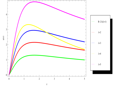
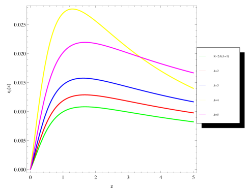
Figure 3: The graphs shows the deviation vector magnitude $\eta(z)$ (left panel) and observer area distance $r_{0}(z)$ (right panel) for null vector field GDE with FLRW background as functions of redshift. The graphs are plotted for $H_{0}=80Km/s/Mpc$, $\Omega_{m0}=0.3$, $\Omega_{r0}=\Omega_{k0}=0$, $\Lambda=1.7.10^{-121}$ and we imposed in equation (57) the initial conditions $\eta(z=0)=0$ and $\eta^{\prime}(z=0)=1$.

We numerically solve the differential equations (69) ($\Lambda CDM$) and (72) (BDR) by plotting the deviation vector magnitude $\eta$ and observer area distance $r_{0}$ as functions of redshift $z$ (Fig. 3). For physical reasons, we will choose the values of $\lambda$ as in Carames ; Carames' . In each panel of (Fig. 3), we observe that the evolution of the deviation $\eta(z)$ and observer area distance $r_{0}(z)$ show similar behavior to those of $\Lambda$CDM. Within this model, we can see as the $\lambda\geqslant 1$ increases and when one goes to the highest values of the redshift $(z\leqslant 0.5)$, the deviation $\eta(z)$ and observer area distance $r_{0}(z)$ decouple each of the model $\Lambda$CDM but still keeps the same place, while for the low values of the redshifts, i.e., for the current day, the BDR model reproduce exactly $\Lambda$CDM. We can conclude that the results are similar to $\Lambda$CDM for all the cases, which means that the above BDR model can be considered remain phenomenologically viable and tested with observational data. We can also observe for small value of redshift $0<z<0.5$, the magnitude of deviation vector $\eta$ presents the same behavior that of $\Lambda CDM$ model ($\lambda=1$). Also, the same behavior was observed for area distance $r_{0}$ at the same level. However, when considering large values of redshift $z>0.5$, we find a gap between the BDR model ($\lambda\neq 1$) and the $\Lambda CDM$ model. This indicates that the BDR model predicts a strong acceleration than $\Lambda CDM$ model for large values of redshift.

V Conclusions

In this paper, we have considered GDE in BDR gravity and calculated the Ricci tensor and Ricci scalar with the modified field equations in BDR gravity. Then, in FLRW universe, corresponding GDE for BDR gravity is obtained. We restricted our attention to extract the GDE for two special cases, namely the fundamental observers and past directed null vector fields. In these two cases, we have found the Raychaudhuri equation, GDE for null vector fields and the diametral angular distance differential for BDR gravity. We have also numerically computed the geodesic deviation ($\eta(z)$) and the area distance ($r_{0}(z)$) from Mattig’s relation for BDR gravity models and compared our results with those of $\Lambda$CDM model (Fig.3).

- (1) C. W. Misner, K. S. Thorne, and J. H. Wheeler. Gravitation. W. H. Freeman and Company, 1973.
- (2) J. L. Synge. On the Deviation of Geodesics and Null Geodesics, Particularly in Relation to the Properties of Spaces of Constant Curvature and Indefinite Line Element, Ann. Math. 35:705 (1934).
- (3) F. A. E. Pirani. On the Physical Significance of the Riemann Tensor. Acta Phys. Polon. 15:389 (1956)
- (4) G. F. R. Ellis and H. Van Elst. Deviation of geodesics in FLRW spacetime geometries (1997), arXiv:gr-qc/9709060v1.
- (5) R. M. Wald, General Relativity ( The University of Chicago Press, 1984).
- (6) E. Poisson, A Relativist’s Toolkit - The Mathematics of Black-Hole Mechanics. Cambridge University Press, 2004.
- (7) C. Corda. Interferometric detection of gravitational waves: the definitive test for General Relativity, Int. J. Mod. Phys. D, 18:2275-2282 (2009) .
- (8) I. Zh. Stefanov, S. S. Yazadjiev, and M. D. Todorov, Scalar-tensor black holes coupled to Born-Infeld nonlinear electrodynamics, Phys. Rev. D 75, 084036 (2007) ; I. Zh. Stefanov, S. S. Yazadjiev, and M. D. Todorov, Scalar-tensor black holes coupled to Euler-Heisenberg nonlinear electrodynamics, Mod. Phys. Lett. A 22, 1217 (2007) ; I. Zh. Stefanov, S. S. Yazadjiev, and M. D. Todorov, Phases of D scalar-tensor black holes coupled to Born-Infeld nonlinear electrodynamics, Mod. Phys. Lett. A 23, 2915 (2008).
- (9) C. Brans and R. H. Dicke, Mach’s principle and a relativistic theory of gravitation, Phys. Rev. 124, 925 (1961).
- (10) C. H. Brans, The roots of scalar-tensor theory: An approximate history, arXiv:gr-qc/0506063.
- (11) K. Nordtvedt Jr, Ap. J. (1970) 1059.
- (12) J. D. Benkestein et al, Phys. Rev. D 18 (1978) 4378.
- (13) J. M. Alimi et al, Phys. Rev. D 53 (1996) 3074..
- (14) Th. P. Sotiriou and V. Faraoni, theories of gravity, Rev. Mod. Phys. 82, 451 (2010).
- (15) C. Mathhiazhagan et al, Class. Quant. Grav. 1 (1984) L29..
- (16) P. M. Garnavich et al, Ap. J. 509 (1998) 74.
- (17) S. Perlmutter et al, Ap. J. 517 (1999) 565.
- (18) A. G. Riess et al, Aston. J. 116 (1999) 74.
- (19) Bodo Geyer , Sergei D. Odintsov , Sergio Zerbini , Phys.Lett. B 460 (1999) 58-62 ; M.C.B. Abdalla, M.E.X. Guimaraes and J.M. Hoff da Silva, European Physical Journal C, 55, 2 (2008) ; Hyungwon Lee, Kyoung Yee Kim and Yun Soo Myung, European Physical Journal C, 71, 3, 1585(2011) ; Lixin Xu, Wenbo Li and Jianbo Lu , European Physical Journal C, 60, 1 (2009).
- (20) É. Cartan, ’’Sur une généralisation de la notion de courbure de Riemann et les espaces à torsion,’’ Acad. Sci. Paris, Comptes Rend. 174 (1922) 593-595
- (21) É. Cartan, “Sur les variétés à connexion affine et la théorie de la relativité généralisée,” Annales Scientifiques de l’École Normale Superieure Sér, 40 (1923) 325-412
- (22) N. Rosen, Theory of gravitation, Physical Review D, 3 (1971) 2317
- (23) J. W. Moffat, ’’Nonsymmetric gravitational theory,’’ Phys. Lett. B 355 (1995) 447.
- (24) J. D. Bekenstein, “Relativistic gravitation theory for the MOND paradigm, Phys. Rev. D 70 (2004) 083509 .
- (25) P. Rastall, ’’Generalization of the einstein theory,’’ Phys. Rev. D 6 (1972) 3357 .
- (26) P. Rastall, “A Theory of Gravity,” Can. J. Phys. 54 (1976) 66.
- (27) H. Bondi and T. Gold, ‘‘The Steady-State Theory of the Expanding Universe,’’ Monthly Notices of the Royal Astronomical Society 108 (1948) 252
- (28) F. Hoyle, A new model for the expanding universe, Monthly Notices of the Royal, Astronomical Society 108 (1948) 372
- (29) P. Jordan, Formation of the Stars and Development of the Universe, Nature 164 (1949) 637.
- (30) Zeldovich, Ya. B. and Pitaevsky, L. P.: Comm. Math, Phys. 23(1971)185.
- (31) Zeldovich, Ya. B. and Starobinsky, A. A.: Sov. Phys. JETP 34(1972)1159.
- (32) Caramês, T.R.P., et al., Eur. Phys. J. C 74, 3145 (2014) .
- (33) Ines G. Salako, Abdul Jawad, Astrophys Space Sci (2015) 359:1-15 .
- (34) A. Guarnizo, L. Castaneda, J. M. Tejeiro, Gen. Rel. Grav.43, 2713 (2011); A. de la Cruz-Dombriz, P. K. S. Dunsby, V. C. Busti, S. Kandhai, Phys. Rev. D 89, 064029 (2014).
- (35) F. Shojai and A. Shojai. Geodesic Congruences in the Palatini Theory. Phys. Rev. D 78:104011 (2008) .
- (36) F. Darabi, M. Mousavi, K. Atazadeh, Phys.Rev. D 91 (2015) 084023.
- (37) E. H. Baffou, M. J. S. Houndjo, M. E. Rodrigues, A. V. Kpadonou, J. Tossa, arXiv:1509.06997.
- (38) M. G. Ganiou , Ines G. Salako, M. J. S. Houndjo, J. Tossa, arXiv:1601.02895
- (39) L. L. Smalley, Variational Principle for a Prototype Rastall Theory of Gravitation, Nuovo Cim. B 80 1 (1984) 42.
- (40) C. E. M. Batista, J. C. Fabris and M. H. Daouda, ‘‘Testing the Rastall’s theory using matter power spectrum,’’ Nuovo Cim. B 125 (2010) 957
- (41) J. C. Fabris, T. C. C. Guio, M. Hamani Daouda and O. F. Piattella, Scalar models for the generalized Chaplygin gas and the structure formation constraints, Grav. Cosmol. 17 (2011) 259.
- (42) J. C. Fabris, M. H. Daouda and O. F. Piattella, ’’Note on the Evolution of the Gravitational Potential in Rastall Scalar Field Theories,’’ Physics Letters B 711, Issues 3–4, ( 2012).
- (43) M. Capone, V. F. Cardone and M. L. Ruggiero, “Accelerating cosmology in Rastall’s theory, Nuovo Cim. B 125 (2011) 1133.
- (44) M. Jamil et al, Phys. Lett. B 694 (2011) 284; M.R. Setare and M. Jamil, Phys. Lett. B 690 (2010).
- (45) G. F. R. Ellis and H. Van Elst. Cosmological models (Cargèse lectures 1998), arXiv:gr-qc/9812046v5.
- (46) D. L. Caceres, L. Castañeda, J. M. Tejeiro. Geodesic Deviation Equation in Bianchi Cosmologies, J. Phys. Conf. Ser. 229:012076 (2010).
- (47) S. Rippl, H. van Elst, R. Tavakol and D. Taylor. Kinematics and dynamics of theories of gravity, Gen. Relativ. Gravit. 28:193 (1996).
- (48) P. Schneider, J. Ehlers and E. E. Falco,Gravitational Lenses, (Springer-Verlag, 1999).
- (49) Y. Bisbar, Phys. Rev. D 86, 127503 (2012), W. Yang, Y. Wu, L. Song, Y. Su, J. Li, D. Zhang, X. Wang, Mod. Phys. Lett. A 26, 191 (2011).