Posterior Dispersion Indices

Abstract

Probabilistic modeling is cyclical: we specify a model, infer its posterior, and evaluate its performance. Evaluation drives the cycle, as we revise our model based on how it performs. This requires a metric. Traditionally, predictive accuracy prevails. Yet, predictive accuracy does not tell the whole story. We propose to evaluate a model through posterior dispersion. The idea is to analyze how each datapoint fares in relation to posterior uncertainty around the hidden structure. We propose a family of posterior dispersion indices (pdi) that capture this idea. A pdi identifies rich patterns of model mismatch in three real data examples: voting preferences, supermarket shopping, and population genetics.

1 Introduction

Probabilistic modeling is a flexible approach to analyzing structured data. Three steps define the approach. First, specify a model; this captures our structural assumptions about the data. Then, we infer the hidden structure; this means computing (or approximating) the posterior. Last, we evaluate the model; this helps build better models down the road.

How do we evaluate models? Decades of reflection have led to deep and varied forays into model checking, comparison, and criticism (Gelman et al., 2013). But a common theme permeates all approaches to model evaluation: the desire to generalize well.

In machine learning, we traditionally employ two complementary tools: predictive accuracy and cross-validation. Predictive accuracy is the target evaluation metric. Cross-validation captures a notion of generalization and justifies holding out data. This simple combination has fueled the development of myriad probabilistic models (Bishop, 2006; Murphy, 2012).

Does predictive accuracy tell the whole story? Predictive accuracy at the datapoint level offers a way to evaluate each observation in the dataset. In this way, pointwise predictive accuracy indicates datapoints that do not match the model well. Yet it does not tell us how the mismatch occurs.

Main idea.  We propose to evaluate probabilistic models through the idea of posterior dispersion, analyzing how each datapoint fares in relation to posterior uncertainty around the hidden structure. To capture this, we propose a family of posterior dispersion indices (pdi). These are per-datapoint quantities, each a variance to mean ratio of the model likelihood with respect to the posterior. A pdi highlights datapoints that exhibit the most uncertainty under the posterior.

Consider a model $p(\boldsymbol{\mathbf{x}},\boldsymbol{\mathbf{\theta}})$ and the likelihood of a datapoint $p(x_{n}\,|\,\boldsymbol{\mathbf{\theta}})$. It depends on some hidden structure $\boldsymbol{\mathbf{\theta}}$ that we seek to uncover. Since $\boldsymbol{\mathbf{\theta}}$ is random, we can view the likelihood as a random variable and ask: how does the likelihood of $x_{n}$ vary with respect to the posterior $p(\boldsymbol{\mathbf{\theta}}\,|\,\boldsymbol{\mathbf{x}})$?

To answer this, we appeal to various forms of dispersion, such as the variance of the likelihood under the posterior. We propose a family of calibrated dispersion criteria of form

pdi $$=\frac{\text{variance of likelihood under posterior}}{\text{mean of likelihood under posterior}}=\frac{\mathbb{V}_{\boldsymbol{\mathbf{\theta}}|\boldsymbol{\mathbf{x}}}[p(x_{n}\,|\,\boldsymbol{\mathbf{\theta}})]}{\mathbb{E}_{\boldsymbol{\mathbf{\theta}}|\boldsymbol{\mathbf{x}}}[p(x_{n}\,|\,\boldsymbol{\mathbf{\theta}})]}$$

Here is a mental picture. Consider a study of human body temperatures. The posterior represents uncertainty around temperature. Imagine a high measurement $T_{\text{fever}}$. Its likelihood varies rapidly across plausible values for $T$. This datapoint is well modeled, but is sensitive to the posterior. Now imagine a zero measurement. This datapoint is poorly modeled, but consistently so: the thermometer is broken. A pdi highlights the first datapoint as a more important type of mismatch than the second.

Section 3 presents an empirical study of model mismatch in three real-world examples: voting preferences, supermarket shopping, and population genetics. In each of these cases, a pdi provides insight into the model and offers concrete directions for improvement.

Related work.  This paper relates to a constellation of ideas from statistical model criticism. pdi bears similarity to anova, which is a frequentist approach to evaluating explanatory variables in linear regression (Davison, 2003). Gelman et al. (1996) cemented the idea of studying predictive accuracy of probabilistic models at the data level; Vehtari et al. (2012) and Betancourt (2015) give up-to-date overviews of these ideas. Recent forays into model criticism, such as Gelman et al. (2014), Vehtari et al. (2014) and Piironen and Vehtari (2015), explore the relationship between cross-validation and information criteria, such as widely applicable information criterion (waic) (Watanabe, 2010; Vehtari et al., 2016). waic offers an intuitive connection to cross validation (Vehtari and Lampinen, 2002; Watanabe, 2015); we draw inspiration from it in this paper too. In the machine learning community, Gretton et al. (2007) and Chwialkowski et al. (2016) developed effective kernel-based methods for independence and goodness-of-fit tests. Recently, Lloyd and Ghahramani (2015) visualized smooth regions of data space that the model fails to explain. In contrast, we focus directly on the datapoints, which can live in high-dimensional spaces that are difficult to visualize.

2 Posterior Dispersion Indices

A posterior dispersion index (pdi) highlights datapoints that exhibit the most uncertainty with respect to the hidden structure of a model. Here is the road map for this section. A small case study illustrates how a pdi gives more insight beyond predictive accuracy. Definitions, theory, and another small analysis give further insight; a straightforward algorithm leads into the empirical study.

2.1 A motivating case study: 44% outliers?

Hayden (2005) considers the number of days each U.S. president stayed in office. Figure 1 plots the data. One-term presidents stay in office for around 1460 days; two-term presidents approximately double that. Yet many presidents deviate from this “two bump” trend.

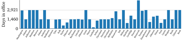
Figure 1: The number of days each U.S. president stayed in office. Typical durations are easy to identify; gray lines indicate one- and two-term stays. Appendix A presents numerical values.

A reasonable model for such data is a mixture of negative binomial distributions. Consider the “second” parameterization of the negative binomial with mean $\mu$ and variance $\mu+\nicefrac{{\mu^{2}}}{{\phi}}$. Posit gamma priors on the (non-negative) latent variables. Set the prior on $\mu$ to match the mean and variance of the data (Robbins, 1964). Choose an uninformative prior on $\phi$. Three mixtures make sense: two for the typical trends and one for the rest.

The complete model is

$$p(\boldsymbol{\mathbf{\pi}}) =\text{Dirichlet}(\boldsymbol{\mathbf{\pi}}\>;\>\alpha=(1,1,1))$$

$$p(\boldsymbol{\mathbf{\mu}}) =\prod_{k=1}^{3}\textrm{Gam}(\mu_{k}\>;\>\text{mean and variance matched to that of data})$$

$$p(\boldsymbol{\mathbf{\phi}}) =\prod_{k=1}^{3}\textrm{Gam}(\phi_{k}\>;\>a=1,\beta=0.01)$$

$$p(x_{n}\,|\,\boldsymbol{\mathbf{\pi}},\boldsymbol{\mathbf{\mu}},\boldsymbol{\mathbf{\phi}}) =\sum_{k=1}^{3}\pi_{k}\text{NB2}(x_{n}\>;\>\mu_{k},\phi_{k}).$$

Fitting this model gives posterior mean estimates $\smash{\widehat{\boldsymbol{\mathbf{\mu}}}=(1461,2896,{\color[rgb]{0.72,0,0}1578})}$ with corresponding $\smash{\widehat{\boldsymbol{\mathbf{\phi}}}=(470,509,{\color[rgb]{0.72,0,0}1.3})}$. The first two clusters describe the two typical term durations, while the third (highlighted in red) is a dispersed negative binomial that attempts to describe the rest of the data.

We compute a pdi (defined in Section 2.2) and the posterior predictive density for each president $p(x_{n}\,|\,\boldsymbol{\mathbf{x}})$. Figure 2 compares both metrics and sorts the presidents according to the pdi.

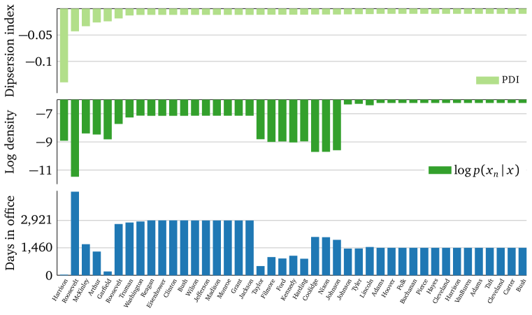
Figure 2: pdi and log predictive accuracy of each president under a mixture of three negative binomials model. Presidents sorted by pdi. The closer to zero, the better. (Code in supplement.)

Some presidents are clear outliers: Harrison [31:natural death], Roosevelt [4452:three terms], and Garfield [199:assassinated]. However, there are 3 presidents with worse predictive accuracy than Harrison: Coolidge, Nixon, and Johnson. A pdi differentiates Harrison from these three by also taking into account the variance of his likelihood with respect to the posterior.

pdi also calls attention to McKinley [1655:assassinated] and Arthur [1260:succeeded Garfield]; this is because they are close to the peaked negative binomial cluster at 1460 but not close enough to have good predictive accuracy. They are datapoints whose likelihoods are rapidly changing with respect to the posterior, like the fever measurement in the introduction.

This case study suggests that predictive probability does not tell the entire story. Datapoints can exhibit low predictive accuracy in different ways. The following two sections define and explain how a pdi captures this effect.

2.2 Definitions

Let $\boldsymbol{\mathbf{x}}=\{x_{n}\}_{1}^{N}$ be a dataset with $N$ observations. A probabilistic model has two parts. The first is the likelihood, $p(x_{n}\,|\,\boldsymbol{\mathbf{\theta}})$. It relates an observation $x_{n}$ to hidden patterns described by a set latent random variables $\boldsymbol{\mathbf{\theta}}$. If the observations are independent and identically distributed, the likelihood of the dataset factorizes as $p(\boldsymbol{\mathbf{x}}\,|\,\boldsymbol{\mathbf{\theta}})=\prod_{n}p(x_{n}\,|\,\boldsymbol{\mathbf{\theta}})$.

The second is the prior density, $p(\boldsymbol{\mathbf{\theta}})$. It captures the structure we expect from the hidden patterns. Combining the likelihood and the prior gives the joint density $p(\boldsymbol{\mathbf{x}},\boldsymbol{\mathbf{\theta}})=p(\boldsymbol{\mathbf{x}}\,|\,\boldsymbol{\mathbf{\theta}})p(\boldsymbol{\mathbf{\theta}})$. Conditioning the joint on the observed data gives the posterior density, $p(\boldsymbol{\mathbf{\theta}}\,|\,\boldsymbol{\mathbf{x}})$.

Treat the likelihood of each datapoint as a function of $\boldsymbol{\mathbf{\theta}}$. To evaluate the model, we analyze how each datapoint fares in relation to the posterior density. Consider these expectations and variances with respect to the posterior,

$$\begin{aligned} \mu(n)&=\mathbb{E}_{\boldsymbol{\mathbf{\theta}}|\boldsymbol{\mathbf{x}}}[p(x_{n}\,|\,\boldsymbol{\mathbf{\theta}})]&\;\mu_{\text{log}}(n)&=\mathbb{E}_{\boldsymbol{\mathbf{\theta}}|\boldsymbol{\mathbf{x}}}[\log p(x_{n}\,|\,\boldsymbol{\mathbf{\theta}})],\\ \sigma^{2}(n)&=\mathbb{V}_{\boldsymbol{\mathbf{\theta}}|\boldsymbol{\mathbf{x}}}[p(x_{n}\,|\,\boldsymbol{\mathbf{\theta}})]&\;\sigma_{\text{log}}^{2}(n)&=\mathbb{V}_{\boldsymbol{\mathbf{\theta}}|\boldsymbol{\mathbf{x}}}[\log p(x_{n}\,|\,\boldsymbol{\mathbf{\theta}})].\end{aligned}$$ (1)

Each includes the likelihood in a slightly different fashion. The first expectation is a familiar object: $\mu(n)$ is the posterior predictive distribution.

A pdi is a ratio of these variances to expectations. Taking the ratio calibrates this quantity for each datapoint. Recall the mental picture from the introduction. The variance of the likelihood under the posterior highlights potential model mismatch; dividing by the mean calibrates this spread to its predictive accuracy.

Related ratios also appear in classical statistics under a variety of forms, such as indices of dispersion (Hoel, 1943), coefficients of variation (Koopmans et al., 1964), or the Fano factor (Fano, 1947). They all quantify dispersion of samples from a random process.

In this paper, we propose and study the widely applicable posterior dispersion index (wapdi),

$$\textsc{wapdi}(n) =\frac{\sigma_{\text{log}}^{2}(n)}{\log\mu(n)}.$$

Its form and name comes from the widely applicable information criterion

waic $$=-\frac{1}{N}\sum_{n}\log\mu(n)+\sigma_{\text{log}}^{2}(n).$$

waic measures generalization error; it asymptotically equates to leave-one-one cross validation (Watanabe, 2010, 2015). wapdi has two advantages; both are practically motivated. First, we hope the reader is computing some estimate of generalization error. Gelman et al. (2014) recommends waic, since it is easy to compute and designed for common machine learning models (Watanabe, 2010). Computing waic gives wapdi for free. Second, the variance is a second-order moment calculation; using the log likelihood gives numerical stability to the computation. (More on computation in Section 2.4.)

wapdi compares the variance of the log likelihood to the log posterior predictive. This gives insight into how the likelihood of a datapoint fares under the posterior distribution of the hidden patterns. We now analyze this in more detail.

2.3 Intuition: not all predictive probabilities are created equal

The posterior predictive density is an expectation, $\mathbb{E}_{\boldsymbol{\mathbf{\theta}}|\boldsymbol{\mathbf{x}}}[p(x_{\text{new}}\,|\,\boldsymbol{\mathbf{\theta}})]=\int\!\!p(x_{\text{new}}\,|\,\boldsymbol{\mathbf{\theta}})p(\boldsymbol{\mathbf{\theta}}\,|\,\boldsymbol{\mathbf{x}})\mathop{}\!\mathrm{d}\boldsymbol{\mathbf{\theta}}.$ Expectations are integrals: areas under a curve. Different likelihood and posterior combinations can lead to similar integrals.

A toy model illustrates this. Consider a gamma likelihood with fixed shape, and place a gamma prior on the rate. The model is

$$p(\beta) =\textrm{Gam}(\beta\>;\>a_{0}=1,b_{0}=1),$$

$$p(\boldsymbol{\mathbf{x}}\,|\,\beta) =\prod_{n=1}^{N}\textrm{Gam}(x_{n}\>;\>a=5,\beta),$$

which gives the posterior $p(\beta\,|\,\boldsymbol{\mathbf{x}})=\textrm{Gam}(\beta\>;\>a=a_{0}+2N,b=b_{0}+\sum_{n}x_{n})$.

Now simulate a dataset of size $N=10$ with $\beta=1$; the data have mean $\nicefrac{{a}}{{\beta}}=5$. Now consider an outlier at $15$. We can find another $x$ value with essentially the same predictive accuracy

$$\log p(x_{1}=0.727\,|\,\boldsymbol{\mathbf{x}}) =-5.633433, \log p(x_{2}=15\,|\,\boldsymbol{\mathbf{x}}) =-5.633428.$$

Yet their wapdi values differ by an order of magnitude

$$\textsc{wapdi}(x_{1}=0.727) =-0.067, \textsc{wapdi}(x_{2}=15) =-0.229.$$

In this case, wapdi highlights $x_{2}=15$ as a more severe outlier than $x_{1}=0.727$, even though they have the same predictive accuracy. What does that mean? Figure 3 depicts the difference.

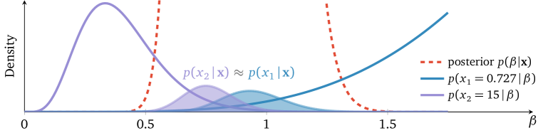
Figure 3: Not all predictive probabilities are created equal. The translucent curves are the two likelihoods multiplied by the posterior (cropped). The posterior predictive $p(x_{1,2}\,|\,\boldsymbol{\mathbf{x}})$ for each datapoint is the area under the curve. While both datapoints have the same predictive accuracy, the likelihood for $x_{2}$ has higher variance under the posterior; $x_{2}$ is more sensitive to the spread of the posterior than $x_{1}$. wapdi captures this effect. (Code in supplement.)

The following lemma explains how wapdi measures this effect.

Lemma 1

If $\log p(x_{n}\,|\,\boldsymbol{\mathbf{\theta}})$ is at least twice differentiable and the posterior $p(\boldsymbol{\mathbf{\theta}}\,|\,\boldsymbol{\mathbf{x}})$ has finite first and second moments, then a first-order Taylor expansion gives

$$\textsc{wapdi}(n) \approx\frac{\left(\log p^{\prime}(x_{n}\,|\,\mathbb{E}_{\boldsymbol{\mathbf{\theta}}|\boldsymbol{\mathbf{x}}}[\boldsymbol{\mathbf{\theta}}])\right)^{2}\mathbb{V}_{\boldsymbol{\mathbf{\theta}}|\boldsymbol{\mathbf{x}}}[\boldsymbol{\mathbf{\theta}}]}{\log\mathbb{E}_{\boldsymbol{\mathbf{\theta}}|\boldsymbol{\mathbf{x}}}[p(x_{n}\,|\,\boldsymbol{\mathbf{\theta}})]}.$$ (2)

Corollary 1

wapdi highlights datapoints whose likelihood is rapidly changing at the posterior mean estimate of the latent variables. ($\mathbb{V}_{\boldsymbol{\mathbf{\theta}}|\boldsymbol{\mathbf{x}}}[\boldsymbol{\mathbf{\theta}}]$ is constant across $n$.)

Looking back at Figure 3, the likelihood $p(x_{2}=15\,|\,\beta)$ indeed changes rapidly under the posterior. wapdi reports the ratio of this rate-of-change to the area under the curve. In this special example, only the numerator matters, since the denominator is the same for both datapoints.

Corollary 2

Equation (2) is zero if and only if the posterior mean coincides with the maximum likelihood estimate of $\boldsymbol{\mathbf{\theta}}$. ($\mathbb{V}_{\boldsymbol{\mathbf{\theta}}|\boldsymbol{\mathbf{x}}}[\boldsymbol{\mathbf{\theta}}]$ is positive for finite $N$.)

For most interesting models, we do not expect such a coincidence. However, in practice, we find wapdi to be close to zero for datapoints that match the model well.

2.4 Computation

Calculating wapdi is straightforward. The only requirement are samples from the posterior. This is precisely the output of an Markov chain Monte Carlo (mcmc) sampling algorithm. (We used the no-U-turn sampler (Hoffman and Gelman, 2014) for the analyses above.) Other inference procedures, such as variational inference, give an analytic approximation to the posterior (Jordan et al., 1999; Blei et al., 2016). Drawing samples from an approximate posterior also works.

Equipped with $S$ samples from the posterior, Monte Carlo integration (Robert and Casella, 1999) gives unbiased estimates of the quantities in Equation (1). The variance of these estimates decreases as $\mathcal{O}(\nicefrac{{1}}{{S}})$; we assume $S$ is sufficiently large to cover the posterior (Gelman et al., 2014). We default to $S=1000$ in our experiments. Algorithm 1 summarizes these steps.

Input: Data $\boldsymbol{\mathbf{x}}=\{\boldsymbol{\mathbf{x}}_{n}\}_{1}^{N}$, model $p(\boldsymbol{\mathbf{x}},\boldsymbol{\mathbf{\theta}})$.

Output: Posterior dispersion index for each datapoint $x_{n}$.

Draw $S$ samples $\{\boldsymbol{\mathbf{\theta}}\}_{1}^{S}$ from posterior (approximation) $p(\boldsymbol{\mathbf{\theta}}\,|\,\boldsymbol{\mathbf{x}})$. for n in 1, 2, …, N do

       Estimate $\mu(n),\mu_{\text{log}}(n),\sigma^{2}(n),\sigma_{\text{log}}^{2}(n)$ from samples $\{\boldsymbol{\mathbf{\theta}}\}_{1}^{S}$. Store these estimates. Return the desired ratio.

end for

Algorithm 1 Calculating posterior dispersion indices.

3 Experimental Study

We now explore three real data examples using modern machine learning models: voting preferences, supermarket shopping, and population genetics.

3.1 Voting preferences: a hierarchical logistic regression model

In 1988, CBS conducted a U.S. nation-wide survey of voting preferences. People indicated their preference towards the Democratic or Republican presidential candidate. Each individual also declared their gender, age, race, education level, and the state they live in; $11\,566$ individuals participated.

Gelman and Hill (2006) study this data through a hierarchical logistic regression model. They begin by modeling gender, race, and state; the state variable has a hierarchical prior. This model is easy to fit using automatic differentiation variational inference (advi) within Stan (Kucukelbir et al., 2015; Carpenter et al., 2015). (Model and inference details in Appendix B.)

vote	r	r	r	r	r	r	r	r	r	r
sex	f	f	f	f	f	f	f	f	f	f
race	b	b	b	b	b	b	b	b	b	b
state	wa	wa	ny	wi	ny	ny	ny	ny	ma	ma

Table 1: Lowest predictive accuracy

vote	d	d	d	d	d	d	r	d	d	d
sex	f	f	f	f	f	m	m	m	m	m
race	w	w	w	w	w	w	w	w	w	w
state	wy	wy	wy	wy	wy	wy	wy	dc	dc	nv

Table 2: Lowest wapdi

Tables 2 and 2 show the individuals with the lowest predictive accuracy and wapdi. The nation-wide trend predicts that females (f) who identify as black (b) have a strong preference to vote democratic (d); predictive accuracy identifies the few individuals who defy this trend. However, there is not much to do with this information; the model identifies a nation-wide trend that correctly describes most female black voters. In contrast, wapdi points to parts of the dataset that the model fails to describe; these are datapoints that we might try to explain better with a revised model.

Most of the individuals with low wapdi live in Wyoming, the District of Columbia, and Nevada. We focus on Wyoming and Nevada. The average wapdi for Wyoming and Nevada are $-0.057$ and $-0.041$; these are baselines that we seek to improve. (The closer to zero, the better.)

Consider expanding the model by modeling age. Introducing age into the model with a hierarchical prior reveals that older voters tend to vote Republican. This helps explain Wyoming voters; their average wapdi drops down from $-0.057$ to $-0.04$; however Nevada’s average wapdi remains unchanged. This means that Nevada’s voters may not follow the national age-dependent trend. Now consider removing age and introducing education in a similar way. Education helps explain voters from both states; the average wapdi for Wyoming and Nevada drop to $-0.041$ and $-0.029$.

wapdi thus captures interesting datapoints beyond what predictive accuracy reports. As expected, predictive accuracy still highlights the same female black voters in both expanded models; wapdi illustrates a deeper way to evaluate this model.

3.2 Supermarket shopping: a hierarchical Poisson factorization model

Market research firm IRi hosts an anonymized dataset of customer shopping behavior at U.S. supermarkets (Bronnenberg et al., 2008). The dataset tracks $136\,584$ “checkout” sessions; each session contains a basket of purchased items. An inventory of $7\,903$ items range across categories such as carbonated beverages, toiletries, and yogurt.

What items do customers tend to purchase together? To study this, consider a hierarchical Poisson factorization (hpf) model (Gopalan et al., 2015). hpf models the quantities of items purchased in each session with a Poisson likelihood; its rate is an inner product between a session’s preferences $\boldsymbol{\mathbf{\theta}}_{s}$ and the item attributes $\boldsymbol{\mathbf{\beta}}$. Hierarchical priors on $\boldsymbol{\mathbf{\theta}}$ and $\boldsymbol{\mathbf{\beta}}$ simultaneously promote sparsity, while accounting for variation in session size and item popularity. Some sessions contain only a few items; others are large purchases. (Model and inference details in Appendix C.)

A $20$-dimensional hpf model discovers intuitive trends. A few stand out. Snack-craving customers like to buy Doritos tortilla chips along with Lay’s potato chips. Morning birds typically pair Cheerios cereal with 2% skim milk. Yoplait fans tend to purchase many different flavors at the same time. Tables 4 and 4 show the top five items in two of these twenty trends.

Item Description	Category
Brand A: 2% skim milk	milk rfg skim/lowfat
Cheerios: cereal	cold cereal
Diet Coke: soda	carbonated beverages
Brand B: 2% skim milk	milk rfg skim/lowfat
Brand C: 2% skim milk	milk rfg skim/lowfat

Table 3: Morning-bird trend

Item Description	Category
Yoplait: raspberry flavor	yogurt rfg
Yoplait: peach flavor	yogurt rfg
Yoplait: strawberry flavor	yogurt rfg
Yoplait: blueberry flavor	yogurt rfg
Yoplait: blackberry flavor	yogurt rfg

Table 4: Yoplait fan trend

Sessions where a customer purchases many items from different categories have low predictive accuracy. This makes sense as these customers do not exhibit a trend; mathematically, there is no combination of item attributes $\boldsymbol{\mathbf{\beta}}$ that explain buying items from disparate categories. For example, the session with the lowest predictive accuracy contains 117 items ranging from coffee to hot dogs.

wapdi highlights an entirely different aspect of the hpf model. Sessions with low wapdi contain similar items but exhibit many purchases of a single item. Table 5 shows an example of a session where a customer purchased 14 blackberry Yoplait yogurts, but only a few of the other flavors.

Item Description	Quantity
Yoplait: blackberry flavor	14
Yoplait: strawberry flavor	2
Yoplait: raspberry flavor	2
Yoplait: peach flavor	1
Yoplait: cherry flavor	1
Yoplait: mango flavor	1

Table 5: A session with low wapdi

This indicates that the Poisson likelihood assumption may not be flexible enough to model customer purchasing behavior. Perhaps a negative binomial likelihood could model this kind of spiked activity better. Another option might be to keep the Poisson likelihood but increase the hierarchy of the probabilistic model; this approach may identify item attributes that explain such purchases. In either case, wapdi identifies a valuable aspect of the data that the hpf struggles to capture: sessions with spiked activity. This is a concrete direction for model revision.

3.3 Population genetics: a mixed membership model

Do all people who live nearby have similar genomes? Not necessarily. Population genetics considers how individuals exhibit ancestral patterns of mutations. Begin with $N$ individuals and $L$ locations on the genome. For each location, report whether each individual reveals a mutation. This gives an ($N\times L$) dataset $\boldsymbol{\mathbf{x}}$ where $x_{nl}\in{0,1,2,3}$. (We assume two specific forms of mutation; 3 encodes a missing observation.)

Mixed membership models offer a way to study this (Pritchard et al., 2000). Assume $K$ ancestral populations $\boldsymbol{\mathbf{\phi}}$; these are the mutation probabilities of each location. Each individual mixes these populations with weights $\boldsymbol{\mathbf{\theta}}$; these are the mixing proportions. Place a beta prior on the mutation probabilities and a Dirichlet prior on the mixing proportions.

We study a dataset of $N=324$ individuals from four geographic locations and focus on $L=13\,928$ locations on the genome. Figure 4 shows how these individuals mix $K=3$ ancestral populations. (Data, model, and inference details in Appendix D.)

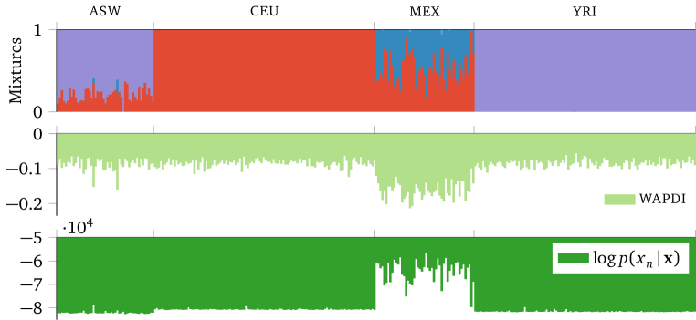
Figure 4: Individuals of African ancestry in southwest U.S. (asw) and Mexican ancestry in Los Angeles (mex) exhibit a mixture of two populations. In contrast, Utah residents with European ancestry (ceu) and members of the Yoruba group in Nigeria (yri) are mostly uniform.

wapdi reveals three interesting patterns of mismatch here. First, individuals with low wapdi have many missing observations; the bottom 10% of wapdi have $1\,344$ missing values, in contrast to $563$ for the lowest 10% of predictive scores. We may consider directly modeling these missing observations.

Second, asw has two individuals with low wapdi; their mutation patterns are outliers within the group. While the average individual reveals 272 mutations away from the median genome, these individuals show 410 and 383 mutations. This points to potential mishaps while gathering or pre-processing the data.

Last, mex exhibits good predictive accuracy, yet low wapdi. Based on predictive accuracy, we may happily accept these patterns. Yet wapdi highlights a serious issue with the inferred populations. The blue and red populations are almost twice as correlated ($0.58$) as the other possible combinations ($0.24$ and $0.2$). In other words, the blue and red populations represent similar patterns of mutations at the same locations. These populations, as they stand, are not necessarily interpretable. Revising the model to penalize correlation may be a direction worth pursuing.

4 Discussion

A posterior dispersion index (pdi) identifies informative forms of model mismatch beyond predictive accuracy. By highlighting which datapoints exhibit the most uncertainty under the posterior, a pdi offers a new perspective into evaluating probabilistic models. Here, we show how the widely applicable posterior dispersion index (wapdi) reveals concrete directions for model improvement across a range of models and applications.

There are several exciting research directions going forward. One is to extend the notion of a pdi to non-exchangeable data. Another is to leverage the bootstrap to extend this idea beyond probabilistic models. Finally, theoretical connections to cross-validation await discovery, while ideas from importance sampling could reduce the variance of pdi computations.

Acknowledgments

We thank David Mimno, Maja Rudolph, Dustin Tran, and Aki Vehtari for their insightful comments. This work is supported by NSF IIS-1247664, ONR N00014-11-1-0651, and DARPA FA8750-14-2-0009.

Appendix A U.S. presidents dataset

Hayden (2005) studies this dataset (and provides a fascinating educational perspective too).

President	Days
Washington	2864
Adams	1460
Jefferson	2921
Madison	2921
Monroe	2921
Adams	1460
Jackson	2921
VanBuren	1460
Harrison	31
Tyler	1427
Polk	1460
Taylor	491
Filmore	967
Pierce	1460
Buchanan	1460
Lincoln	1503
Johnson	1418
Grant	2921
Hayes	1460
Garfield	199
Arthur	1260
Cleveland	1460
Harrison	1460
Cleveland	1460
McKinley	1655
Roosevelt	2727
Taft	1460
Wilson	2921
Harding	881
Coolidge	2039
Hoover	1460
Roosevelt	4452
Truman	2810
Eisenhower	2922
Kennedy	1036
Johnson	1886
Nixon	2027
Ford	895
Carter	1461
Reagan	2922
Bush	1461
Clinton	2922
Bush	1110

Table 6: Presidents of the United States of America: days in office.

Appendix B Hierarchical logistic regression model

Hierarchical logistic regression models classification tasks in an intuitive way. We study three variants of Gelman and Hill (2006)’s model for the 1988 CBS United States election survey dataset.

First model: no age or education.

The likelihood of voting Republican is

$$\Pr(y_{n}=1) =\text{sigmoid}\bigg{(}\beta^{\text{female}}\cdot\text{female}_{n}+\beta^{\text{black}}\cdot\text{black}_{n}+\alpha^{\text{state}}_{s[n]}\bigg{)},$$

with priors

$$\alpha^{\text{state}}_{j} \sim\mathcal{N}\left(\mu_{\text{state}}\,,\,\sigma_{\text{state}}\right)$$

$$\mu_{\text{state}} \sim\mathcal{N}(0,10)$$

$$\sigma_{\text{state}} \sim\mathcal{N}(0,10)$$

$$\boldsymbol{\mathbf{\beta}} \sim\mathcal{N}(0,1).$$

Second model: with age.

The likelihood of voting Republican is

$$\Pr(y_{n}=1) =\text{sigmoid}\bigg{(}\beta^{\text{female}}\cdot\text{female}_{n}+\beta^{\text{black}}\cdot\text{black}_{n}+\alpha^{\text{state}}_{s[n]}+\alpha^{\text{age}}_{a[n]}\bigg{)},$$

with priors

$$\alpha^{\text{state}}_{j} \sim\mathcal{N}\left(\mu_{\text{state}}\,,\,\sigma_{\text{state}}\right)$$

$$\mu_{\text{state}} \sim\mathcal{N}(0,10)$$

$$\sigma_{\text{state}} \sim\mathcal{N}(0,10)$$

$$\alpha^{\text{age}}_{j} \sim\mathcal{N}\left(\mu_{\text{age}}\,,\,\sigma_{\text{age}}\right)$$

$$\mu_{\text{age}} \sim\mathcal{N}(0,10)$$

$$\sigma_{\text{age}} \sim\mathcal{N}(0,10)$$

$$\boldsymbol{\mathbf{\beta}} \sim\mathcal{N}(0,1).$$

Third model: with education.

The likelihood of voting Republican is

$$\Pr(y_{n}=1) =\text{sigmoid}\bigg{(}\beta^{\text{female}}\cdot\text{female}_{n}+\beta^{\text{black}}\cdot\text{black}_{n}+\alpha^{\text{state}}_{s[n]}+\alpha^{\text{edu}}_{a[n]}\bigg{)},$$

with priors

$$\alpha^{\text{state}}_{j} \sim\mathcal{N}\left(\mu_{\text{state}}\,,\,\sigma_{\text{state}}\right)$$

$$\mu_{\text{state}} \sim\mathcal{N}(0,10)$$

$$\sigma_{\text{state}} \sim\mathcal{N}(0,10)$$

$$\alpha^{\text{edu}}_{j} \sim\mathcal{N}\left(\mu_{\text{edu}}\,,\,\sigma_{\text{edu}}\right)$$

$$\mu_{\text{edu}} \sim\mathcal{N}(0,10)$$

$$\sigma_{\text{edu}} \sim\mathcal{N}(0,10)$$

$$\boldsymbol{\mathbf{\beta}} \sim\mathcal{N}(0,1).$$

Appendix C Hierarchical Poisson factorization model

Hierarchical Poisson factorization models a matrix of counts as a low-dimensional inner product. (Gopalan et al., 2015) present the model in detail along with an efficient variational inference algorithm for inference. We summarize the model below.

Model.

Consider a $U\times I$ dataset, with non-negative integer elements $x_{ui}$. It helps to think of $u$ as an index over “users” and $i$ as an index over “items”.

The likelihood for each measurements is

$$p(x_{ui}) =\text{Poisson}(x_{ui}\>;\>\boldsymbol{\mathbf{\theta}}_{u}^{\top}\boldsymbol{\mathbf{\beta}}_{i})$$

where $\boldsymbol{\mathbf{\theta}}$ is a $U\times K$ matrix of non-negative real-valued latent variables; it represents “user preferences”. Similarly, $\boldsymbol{\mathbf{\beta}}$ is a $K\times I$ matrix of non-negative real-valued latent variables; it represents “item attributes”.

The priors for these variables are

$$p(\theta_{uk}) =\textrm{Gam}(\theta_{uk}\>;\>a,\xi_{u})$$

$$p(\beta_{ki}) =\textrm{Gam}(\beta_{ki}\>;\>c,\eta_{i})$$

where $\boldsymbol{\mathbf{\xi}}$ is a $U$ vector of non-negative real-valued latent variables; it represents “user activity”. Similarly, $\boldsymbol{\mathbf{\eta}}$ is a $I$ vector of non-negative real-valued latent variables; it represents “item popularity”.

The prior for these hierarchical latent variable are

$$p(\xi_{u}) =\textrm{Gam}(\xi_{u}\>;\>a^{\prime},\nicefrac{{a^{\prime}}}{{b^{\prime}}})$$

$$p(\eta_{i}) =\textrm{Gam}(\eta_{i}\>;\>c^{\prime},\nicefrac{{c^{\prime}}}{{d^{\prime}}}).$$

Parameters for IRi analysis.

The parameters we used were

$$K =20$$

$$a =\nicefrac{{0.3}}{{\sqrt{K}}}$$

$$c =\nicefrac{{0.3}}{{\sqrt{K}}}$$

$$a^{\prime} =1.5$$

$$b^{\prime} =0.3$$

$$c^{\prime} =1.5$$

$$d^{\prime} =0.3.$$

Inference. We used the coordinate ascent variational inference algorithm provided by the authors of (Gopalan et al., 2015).

Appendix D Population genetics data and model

Population genetics studies ancestral trends of genomic mutations. Consider $N$ individuals and $L$ locations on the genome. For each location, we measure whether each individual reveals a mutation. This gives an ($N\times L$) dataset $\boldsymbol{\mathbf{x}}$ where $x_{nl}\in{0,1,2,3}$. (We assume two specific forms of mutation; 3 encodes a missing observation.)

Model. Pritchard et al. (2000) propose a probabilistic model for this kind of data. Represent $K$ ancestral populations with a latent variable $\boldsymbol{\mathbf{\phi}}$. This is a $(K\times L)$ matrix of mutation probabilities. Place a beta prior for each probability. Each individual mixes these populations. Denote this with another latent variable $\boldsymbol{\mathbf{\theta}}$. This is a $(N\times K)$ matrix of mixture proportions. Place a Dirichlet prior for each individual. The likelihood of each mutation is a $K$-mixture of categorical distributions.

Data. We study a subset of the Hapmap 3 dataset from (Mimno et al., 2015). This includes $N=324$ individuals and $L=13\,928$ locations on the genome. Four geographic regions are represented: 49 asw, 112 ceu, 50 mex, and 113 yri. Mimno et al. (2015) expect this data to exhibit at most $K=3$ ancestral populations; the full Hapmap 3 dataset exhibits $K=6$ populations.

In more detail, this data studies single-nucleotide polymorphisms (snps). The data is pre-processed from the raw genetic observations such that:

• non-snps are removed (i.e. genes with more than one location changed),

• snps with low entropy compared to the dominant mutation at each location are removed,

• snps that are too close to each other on the genome are removed.

Inference. We use the fastSTRUCTURE software suite (Raj et al., 2014) to perform variational inference. We use the default parameters and only specify $K=3$.

References

- Betancourt (2015) Betancourt, M. (2015). A unified treatment of predictive model comparison. arXiv preprint arXiv:1506.02273.
- Bishop (2006) Bishop, C. M. (2006). Pattern Recognition and Machine Learning. Springer New York.
- Blei et al. (2016) Blei, D. M., Kucukelbir, A., and McAuliffe, J. D. (2016). Variational inference: a review for statisticians. arXiv preprint arXiv:1601.00670.
- Bronnenberg et al. (2008) Bronnenberg, B. J., Kruger, M. W., and Mela, C. F. (2008). The IRi marketing data set. Marketing Science, 27(4).
- Carpenter et al. (2015) Carpenter, B., Gelman, A., Hoffman, M., Lee, D., Goodrich, B., Betancourt, M., Brubaker, M. A., Guo, J., Li, P., and Riddell, A. (2015). Stan: a probabilistic programming language. JSS.
- Chwialkowski et al. (2016) Chwialkowski, K., Strathmann, H., and Gretton, A. (2016). A kernel test of goodness of fit. arXiv preprint arXiv:1602.02964.
- Davison (2003) Davison, A. C. (2003). Statistical models. Cambridge University Press.
- Fano (1947) Fano, U. (1947). Ionization yield of radiations II. Physical Review, 72(1):26.
- Gelman et al. (2013) Gelman, A., Carlin, J. B., Stern, H. S., Dunson, D. B., Vehtari, A., and Rubin, D. B. (2013). Bayesian Data Analysis. CRC Press.
- Gelman and Hill (2006) Gelman, A. and Hill, J. (2006). Data analysis using regression and multilevel/hierarchical models. Cambridge University Press.
- Gelman et al. (2014) Gelman, A., Hwang, J., and Vehtari, A. (2014). Understanding predictive information criteria for Bayesian models. Statistics and Computing, 24(6):997–1016.
- Gelman et al. (1996) Gelman, A., Meng, X.-L., and Stern, H. (1996). Posterior predictive assessment of model fitness via realized discrepancies. Statistica sinica, 6(4):733–760.
- Gopalan et al. (2015) Gopalan, P., Hofman, J. M., and Blei, D. M. (2015). Scalable recommendation with hierarchical Poisson factorization. UAI.
- Gretton et al. (2007) Gretton, A., Fukumizu, K., Teo, C. H., Song, L., Schölkopf, B., and Smola, A. J. (2007). A kernel statistical test of independence. In NIPS.
- Hayden (2005) Hayden, R. W. (2005). A dataset that is 44% outliers. J Stat Educ, 13(1).
- Hoel (1943) Hoel, P. G. (1943). On indices of dispersion. The Annals of Mathematical Statistics, 14(2):155–162.
- Hoffman and Gelman (2014) Hoffman, M. D. and Gelman, A. (2014). The No-U-Turn sampler. JMLR, 15(1):1593–1623.
- Jordan et al. (1999) Jordan, M. I., Ghahramani, Z., Jaakkola, T. S., and Saul, L. K. (1999). An introduction to variational methods for graphical models. Machine Learning, 37(2):183–233.
- Koopmans et al. (1964) Koopmans, L. H., Owen, D. B., and Rosenblatt, J. (1964). Confidence intervals for the coefficient of variation for the normal and log normal distributions. Biometrika, 51(1/2):25–32.
- Kucukelbir et al. (2015) Kucukelbir, A., Ranganath, R., Gelman, A., and Blei, D. M. (2015). Automatic variational inference in Stan. NIPS.
- Lloyd and Ghahramani (2015) Lloyd, J. R. and Ghahramani, Z. (2015). Statistical model criticism using kernel two sample tests. In NIPS.
- Mimno et al. (2015) Mimno, D., Blei, D. M., and Engelhardt, B. E. (2015). Posterior predictive checks to quantify lack-of-fit in admixture models of latent population structure. Proceedings of the National Academy of Sciences, 112(26).
- Murphy (2012) Murphy, K. P. (2012). Machine Learning: a Probabilistic Perspective. MIT Press.
- Piironen and Vehtari (2015) Piironen, J. and Vehtari, A. (2015). Comparison of Bayesian predictive methods for model selection. arXiv preprint arXiv:1503.08650.
- Pritchard et al. (2000) Pritchard, J. K., Stephens, M., and Donnelly, P. (2000). Inference of population structure using multilocus genotype data. Genetics, 155(2):945–959.
- Raj et al. (2014) Raj, A., Stephens, M., and Pritchard, J. K. (2014). fastSTRUCTURE: variational inference of population structure in large SNP data sets. Genetics, 197(2):573–589.
- Robbins (1964) Robbins, H. (1964). The empirical Bayes approach to statistical decision problems. Annals of Mathematical Statistics.
- Robert and Casella (1999) Robert, C. P. and Casella, G. (1999). Monte Carlo statistical methods. Springer.
- Vehtari et al. (2016) Vehtari, A., Gelman, A., and Gabry, J. (2016). Practical Bayesian model evaluation using leave-one-out cross-validation and WAIC. arXiv preprint arXiv:1507.04544.
- Vehtari and Lampinen (2002) Vehtari, A. and Lampinen, J. (2002). Bayesian model assessment and comparison using cross-validation predictive densities. Neural Computation, 14(10):2439–2468.
- Vehtari et al. (2012) Vehtari, A., Ojanen, J., et al. (2012). A survey of Bayesian predictive methods for model assessment, selection and comparison. Statistics Surveys, 6:142–228.
- Vehtari et al. (2014) Vehtari, A., Tolvanen, V., Mononen, T., and Winther, O. (2014). Bayesian leave-one-out cross-validation approximations for gaussian latent variable models. arXiv preprint arXiv:1412.7461.
- Watanabe (2010) Watanabe, S. (2010). Asymptotic equivalence of Bayes cross validation and widely applicable information criterion in singular learning theory. JMLR, 11:3571–3594.
- Watanabe (2015) Watanabe, S. (2015). Bayesian cross validation and WAIC for predictive prior design in regular asymptotic theory. arXiv preprint arXiv:1503.07970.