A local characterization for constant curvature metrics in 2-dimensional Lorentz manifolds

Abstract

In this paper we define Fermi-type coordinates in a $2-$dimensional Lorentz manifold, and use this coordinate system to provide a local characterization of constant Gaussian curvature metrics for such manifolds, following a classical result from Riemann. We then exhibit particular isometric immersions of such metrics in the pseudo-Riemannian ambients $\mathbb{L}^{3}\equiv\mathbb{R}^{3}_{1}$ and $\mathbb{R}^{3}_{2}$.

MSC 2010: Primary: 53B30
Keywords: Lorentz metrics, Constant Gaussian curvature, pseudo-Riemannian surfaces

1 Introduction

Constant sectional curvature metrics on pseudo-Riemannian manifolds appear naturally in physics as some of the solutions of Einstein’s equation in vacuum

$$R_{\mu\nu}-\frac{1}{2}Rg_{\mu\nu}+\Lambda g_{\mu\nu}=0.$$

If the cosmological constant $\Lambda$ is positive a particular solution is the de Sitter metric; if $\Lambda=0$, it is the Lorentz-Minkowski metric; if $\Lambda$ is negative, it is the anti-de Sitter metric.

In $3-$dimensional Lorentz-Minkowski space, surfaces with constant Gaussian curvature have been studied under a diverse set of hypotheses with different techniques as in [1], [2] and [3].

The local classification of pseudo-Riemannian metrics of index $s$ and constant sectional curvature on $n-$dimensional manifolds is given by the following classical result, known as Riemann’s theorem (see [4, pp. 69]).

Theorem 1.1 (Riemann).

Let $M$ be a pseudo-Riemannian manifold of dimension $n\geq 2$ and let $K$ be a real number. Then the following conditions are equivalent:

1. $M$ is of constant curvature $K$.

2. If $x\in M$, then there are local coordinates $u^{i}$ on a neighborhood of $x$ in which the metric is given by

   $${\rm d}s^{2}=\frac{\epsilon_{1}{\rm d}u^{1}\otimes{\rm d}u^{1}+\ldots+\epsilon_{n}{\rm d}u^{n}\otimes{\rm d}u^{n}}{\left(1+\frac{K}{4}\sum\epsilon_{i}(u^{i})^{2}\right)^{2}},\quad\epsilon_{i}=\pm 1.$$

3. If $x\in M$, then $x$ has a neighborhood which is isometric to an open set on some $\mathbb{S}^{n}_{s}$ if $K>0$, $\mathbb{R}^{n}_{s}$ if $K=0$, $\mathbb{H}^{n}_{s}$ if $K<0$.

In the previous statement we have

$$\mathbb{R}^{n}_{s} =\big{(}\mathbb{R}^{n},\langle{\cdot,\cdot}\rangle_{s}\big{)}$$

$$\mathbb{S}^{n}_{s} =\big{\{}x\in\mathbb{R}^{n+1}_{s}:\langle{x,x}\rangle_{s}=1\big{\}}$$

$$\mathbb{H}^{n}_{s} =\big{\{}x\in\mathbb{R}^{n+1}_{s+1}:\langle{x,x}\rangle_{s+1}=-1\big{\}},$$

where

$$\langle{x,y}\rangle_{s}=\sum\limits_{i=1}^{n-s}x^{i}y^{i}-\sum\limits_{i=n-s+1}^{n}x^{i}y^{i},$$

for any $x=(x^{1},\ldots,x^{n})$ and $y=(y^{1},\ldots,y^{n})$ in $\mathbb{R}^{n}$.

When $s=0$ we have $\mathbb{R}^{n}_{0}=\mathbb{R}^{n}$, the usual Euclidean space and $\mathbb{S}^{n}_{0}=\mathbb{S}^{n}$, the standard Euclidean unit sphere. Furthermore, if $s=1$ we have $\mathbb{R}^{n}_{1}=\mathbb{L}^{n}$, the Lorentz-Minkowski space; $\mathbb{S}^{n}_{1}$, the de Sitter space (eventually denoted by $dS_{n}$); $\mathbb{H}^{n}_{0}=\mathbb{H}^{n}$, the usual hyperbolic space with $x_{n+1}>0$ and $\mathbb{H}^{n}_{1}$ the anti-de Sitter space (eventually denoted by $AdS_{n}$).

In particular, when $n=2$ and $s=0$ we have the following result.

Theorem 1.2.

A surface with $K=0$ is locally isometric to the plane, with $K=1$ is locally isometric to the unit sphere and with $K=-1$ is locally isometric to the hyperbolic plane.

In this work we show a simpler proof of the above theorem when $n=2$ and $s=1$, using Fermi-type coordinates. More precisely we have:

Theorem 1.3.

Let $M$ be a $2-$dimensional pseudo-Riemannian manifold of constant curvature$K\in\{-1,0,1\}$. Then one and only one of the following holds:

1. if $K=0$ then $M$ is locally isometric to Lorentz-Minkowski plane $\mathbb{L}^{2}$, with metric expressed in Fermi-type coordinates as ${\rm d}s^{2}=-{\rm d}u^{2}+{\rm d}v^{2}$ or ${\rm d}s^{2}={\rm d}\tau^{2}-{\rm d}\vartheta^{2}$;

2. if $K=1$ then $M$ is locally isometric to the de Sitter space $\mathbb{S}^{2}_{1}$, with metric expressed in Fermi-type coordinates as ${\rm d}s^{2}=-{\rm d}u^{2}+\cosh^{2}u\,{\rm d}v^{2}$ or ${\rm d}s^{2}={\rm d}\tau^{2}-\cos^{2}\tau\,{\rm d}\vartheta^{2}$;

3. if $K=-1$ then $M$ is locally isometric to the anti-de Sitter space $\mathbb{H}^{2}_{1}$. In this case the metric is expressed in Fermi-type coordinates as ${\rm d}s^{2}=-{\rm d}u^{2}+\cos^{2}u\,{\rm d}v^{2}$ or ${\rm d}s^{2}={\rm d}\tau^{2}-\cosh^{2}\tau\,{\rm d}\vartheta^{2}$;

2 Notation and Preliminaries

Firstly, we establish some notation and recall some standard definitions and results from pseudo-Riemannian geometry.

A pseudo-Riemannian manifold $(M^{n},\langle{\cdot,\cdot}\rangle)$ where $\langle{\cdot,\cdot}\rangle$ has index $1$ will be called a Lorentz manifold. In a Lorentz manifold, a tangent vector $X_{p}\in T_{p}M$ is

• spacelike if $\langle{X_{p},X_{p}}\rangle>0$ or if $X_{p}=0$;

• timelike if $\langle{X_{p},X_{p}}\rangle<0$;

• lightlike if $\langle{X_{p},X_{p}}\rangle=0$ but $X_{p}\neq 0$.

Every tangent vector is of exactly one of the above causal types. The notion of causal type extends to curves in $M$ in a natural way: if $\gamma\colon I\to M$ is a curve, then $\gamma$ is said to be of one of the three causal types above if all its tangent vectors $\gamma^{\prime}(t)$ share that causal type.

Recall that a geodesic in $M$ is a curve $\gamma\colon I\to M$ such that $\nabla_{\gamma^{\prime}(t)}\gamma^{\prime}=0$ for all $t\in I$, where $\nabla$ is the Levi-Civita connection of the metric, or equivalently (see [5, p. 67]), if in all local coordinates $(u^{1},\cdots,u^{n})$ we have

$$\ddot{u}^{k}+\sum_{i,j=1}^{n}\Gamma_{ij}^{k}\dot{u}^{i}\dot{u}^{j}=0,\mbox{ for all $k\in\{1,\ldots,n\}$,}$$ (2.1)

where the dots denote the derivatives of the coordinates of $\gamma$ with respect to the curve parameter and the $\Gamma_{ij}^{k}$ are the Christoffel symbols of the metric in the coordinates chosen. We also have that geodesics do not change causal type, since

$$\frac{{\rm d}}{{\rm d}t}\langle{\gamma^{\prime}(t),\gamma^{\prime}(t)}\rangle=2\langle{\gamma^{\prime}(t),\nabla_{\gamma^{\prime}(t)}\gamma^{\prime}}\rangle=0.$$

It is also easy to see that any non-lightlike curve has a unit-speed reparametrization.

If $M$ is $2-$dimensional, and $(u,v)$ are local coordinates in $M$, we express the metric $\langle{\cdot,\cdot}\rangle$ in these coordinates as:

$${\rm d}s^{2}=E\,{\rm d}u^{2}+2F\,{\rm d}u\,{\rm d}v+G\,{\rm d}v^{2},$$

where

$$E=\langle{\partial_{u},\partial_{u}}\rangle,\quad F=\langle{\partial_{u},\partial_{v}}\rangle,\quad G=\langle{\partial_{v},\partial_{v}}\rangle$$

are the the coefficients of the metric (first fundamental form) in the coordinates $(u,v)$.

On the following we establish some results about $2-$dimensional Lorentz manifolds (henceforth called Lorentz surfaces) starting with an analogous result to the existence of orthogonal coordinates for Riemannian surfaces.

Lemma 2.1.

Let $X$ and $Y$ be linearly independent vector fields in a neighborhood of a point $p$ in a $2-$dimensional smooth manifold. There exists a coordinate system $(u,v)$ at $p$ such that $\partial_{u}=\lambda X$ and $\partial_{v}=\mu Y$.

Proof.

We are looking for smooth positive functions $\lambda$ and $\mu$ such that the Lie bracket $[\lambda X,\mu Y]$ vanishes, since by Frobenius’ theorem we will be able to find local coordinates $(u,v)$ in $M$ satisfying $\partial_{u}=\lambda X$ and $\partial_{v}=\mu Y$. Writing $[X,Y]=fX+gY$ for suitable smooth functions $f$ and $g$ and using the standard properties of Lie brackets leads to

$$0=[\lambda X,\mu Y]=\big{(}\lambda\mu f-\mu Y(\lambda)\big{)}X+\big{(}\lambda\mu g+\lambda X(\mu)\big{)}Y,$$

that is

$$Y(\lambda)=\lambda f\quad\mbox{and}\quad-X(\mu)=\mu g.$$ (2.2)

If $(x,y)$ is any coordinate system at $p$ then we may write $X=a\partial_{x}+b\partial_{y}$ and $Y=c\partial_{x}+d\partial_{y}$, where $a,b,c$ and $d$ are smooth functions such that $ad-bc\neq 0$ and $(a^{2}+b^{2})(c^{2}+d^{2})\neq 0$. Hence we may write

$$X(\mu)=a\mu_{x}+b\mu_{y}\quad\mbox{and}\quad Y(\lambda)=c\lambda_{x}+d\lambda_{y}$$

so that equations (2.2) become

$$\begin{cases}c\dfrac{\lambda_{x}}{\lambda}+d\dfrac{\lambda_{y}}{\lambda}=f,\\[5.0pt] a\dfrac{\mu_{x}}{\mu}+b\dfrac{\mu_{y}}{\mu}=g.\end{cases}$$

Let $h_{1}(x,y)=\ln\big{(}\lambda(x,y)\big{)}$ and $h_{2}(x,y)=\ln\big{(}\mu(x,y)\big{)}$. With this, the equations above are written as

$$\begin{cases}c(x,y)(h_{1})_{x}(x,y)+d(x,y)(h_{1})_{y}(x,y)=f(x,y),\\[5.0pt] a(x,y)(h_{2})_{x}(x,y)+b(x,y)(h_{2})_{y}(x,y)=g(x,y),\end{cases}$$

which are two linear first order PDEs, that have solutions due to the condition $ad-bc\neq 0$. Hence we have found $\lambda=e^{h_{1}}$ and $\mu=e^{h_{2}}$ as desired. ∎

In the case of a Lorentz surface $M$, lemma 2.1 ensures that we can, at least locally, write the metric on $M$ as

$${\rm d}s^{2}=E\,{\rm d}u^{2}+G\,{\rm d}v^{2},$$ (2.3)

where $E$ and $G$ are smooth functions such that $EG<0$. To see this, apply the lemma for two non-lightlike and non-zero orthogonal vector fields of opposite causal characters.

Lemma 2.2.

In this setting the Gaussian curvature of the metric is

$$K=\frac{-1}{\sqrt{|EG|}}\left(\epsilon_{1}\left(\frac{(\sqrt{|G|})_{u}}{\sqrt{|E|}}\right)_{u}+\epsilon_{2}\left(\frac{(\sqrt{|E|})_{v}}{\sqrt{|G|}}\right)_{v}\right),$$ (2.4)

where $\epsilon_{1}$ (resp. $\epsilon_{2}$) is $1$ or $-1$ if $\partial_{u}$ (resp. $\partial_{v}$) is spacelike or timelike.

For a proof of the lemma above see [6, p. 54].

3 Fermi-type coordinates and its properties

From equation (2.1) one sees that given a point $p\in M$ and any unit vector $w\in T_{p}M$ there exists a unique geodesic $\gamma:I\to M$ passing through $p$ with velocity $w$.

We can use this fact to exhibit a local parametrisation of $M$ known, in Euclidean case, as Fermi parametrisation (see [7, p. 275] and [8, p. 192]). For a Lorentz surface we have distinct Fermi-type parametrisations, according to the causal type of the vector $w=\gamma^{\prime}(0)\in T_{p}M$. In order to obtain a regular parametrisation we avoid lightlike geodesics. The construction is the same in both remaining cases and it is done as follows:

Fix an unit speed geodesic $\gamma\colon I\to M$. For each $\gamma(v)\in M$ consider the unit speed geodesic $\gamma_{v}:J_{v}\to M$ intersecting $\gamma$ orthogonally in $\gamma_{v}(0)=\gamma(v)$. Set the map ${\bf x}$ as ${\bf x}(u,v)=\gamma_{v}(u)$, for each $v\in I$ and $u\in J_{v}$.

Recall that geodesics have constant causal type, that is, if $\gamma$ is spacelike (resp. timelike) at some point, $\gamma$ will be spacelike (resp. timelike) everywhere. Therefore all of the $\gamma_{v}$ will be timelike (resp. spacelike), since $\big{\{}\gamma^{\prime}(v),\gamma^{\prime}_{v}(0)\big{\}}$ is an orthonormal basis of $T_{\gamma(v)}M$, for all $v\in I$.

Proposition 3.1.

${\bf x}$ is regular in some open neighborhood of $\gamma(I)\subset M$.

Proof.

We show that ${\bf x}_{u}$ e ${\bf x}_{v}$ are linearly independent in some neighborhood of $(0,v)$, for all $v\in I$. It suffices to note that

$$F(0,v)=\langle{\bf x}_{u}(0,v),{\bf x}_{v}(0,v)\rangle=\langle\gamma_{v}^{\prime}(0),\gamma^{\prime}(v)\rangle=0.$$

Then ${\bf x}_{u}(0,v)$ e ${\bf x}_{v}(0,v)$ are orthogonal along $\gamma(I)$, hence linearly independent (since they are not lightlike) in some open neighborhood of it in $M$. ∎

Proposition 3.2.

In this coordinate system the metric of $M$ is given by

$${\rm d}s^{2}=-\epsilon_{\gamma}\,{\rm d}u^{2}+G\,{\rm d}v^{2}$$ (3.1)

where $\epsilon_{\gamma}$ is $1$ if $\gamma$ is spacelike or $-1$ if timelike.

Proof.

All $\gamma_{v}$ are unit speed curves with the same causal type $\epsilon_{\gamma_{v}}$. We have

$$E(u,v)=\langle{\bf x}_{u}(u,v),{\bf x}_{u}(u,v)\rangle=\langle\gamma^{\prime}_{v}(u),\gamma^{\prime}_{v}(u)\rangle=\epsilon_{\gamma_{v}}.$$

Now $\epsilon_{\gamma}\epsilon_{\gamma_{v}}=-1$ for all $v$, since $M$ is $2-$dimensional, the metric is non-degenerate and has index $1$. Hence $E(u,v)=-\epsilon_{\gamma}$.

Also, by construction, $F(0,v)=0$ for all $v$. It remains to show that $F$ does not depend on $u$. Fixing $v_{0}\in I$, note that $\gamma_{v_{0}}(u)={\bf x}(u,v_{0})$ has coordinates $u^{1}=u$ e $u^{2}=v_{0}$, so making $k=2$ in (2.1) yields $\Gamma_{11}^{2}=0$.

Writing $(g_{ij})=\begin{pmatrix}E&F\\ F&G\end{pmatrix}$ and its inverse as $(g^{ij})$, the expressions of Christoffel in terms of these objects are (see [5, p. 62]):

$$\Gamma_{ij}^{k}=\sum_{r=1}^{2}\frac{1}{2}g^{kr}\left(\frac{\partial g_{ir}}{\partial u^{j}}+\frac{\partial g_{jr}}{\partial u^{i}}-\frac{\partial g_{ij}}{\partial u^{r}}\right).$$ (3.2)

Setting $k=2$ and $i=j=1$ in equation (3.2) leads to $g^{22}F_{u}(u,v_{0})=0$. It is clear that $g^{22}=\dfrac{-\epsilon_{\gamma}}{\det(g_{ij})}\neq 0$, hence $F_{u}(u,v_{0})=0$, that is, $F(u,v)=0$. ∎

Remark 3.3.

Since $G(0,v)=\epsilon_{\gamma}\neq 0$ and $G$ is continuous, we can assume that the neighborhood of $\gamma(I)\subseteq M$ found on proposition 3.1 (reducing it if necessary) is such that $G$ and $\epsilon_{\gamma}$ have the same sign.

Lemma 3.4.

In the same setting of the previous proposition, the Gaussian curvature of the metric ${\rm d}s^{2}=-\epsilon_{\gamma}\,{\rm d}u^{2}+G\,{\rm d}v^{2}$ is

$$K=\epsilon_{\gamma}\frac{(\sqrt{|G|})_{uu}}{\sqrt{|G|}}.$$ (3.3)

Proof.

Make $E=-\epsilon_{\gamma}$ in (2.4). ∎

Lemma 3.5.

$G_{u}(0,v)=0$ for each $v$.

Proof.

Using the same notation in the proof of proposition 3.2, observing that $\gamma(v)=\gamma_{v}(0)={\bf x}(0,v)$ has coordinates $u^{1}=0$, $u^{2}=u$, making $k=1$ in (2.1) we obtain $\Gamma_{22}^{1}=0$. Then, setting $k=1$ and $i=j=2$ in (3.2) gives $G_{u}(0,v)=0$, since $g^{11}=\dfrac{G}{\det(g_{ij})}$. ∎

Remark 3.6.

We observe that there exists two Fermi-type coordinates:

• spacelike Fermi-type coordinates, when the fixed geodesic $\gamma$ is spacelike, that is, $\epsilon_{\gamma}=1$;

• timelike Fermi-type coordinates, when the fixed geodesic $\gamma$ is timelike, that is, $\epsilon_{\gamma}=-1$.

To avoid confusion we will denote the parameters in the timelike Fermi-type coordinates by $(\tau,\vartheta)$.

4 Proof of the Main Result

At this point we are able to prove the main result of this work, providing a local classification of metrics with constant curvature dependng on the chosen Fermi-type coordinates. We work with the possible values for $K$.

1. $K=0$: in this case equation (3.3) becomes

   $$\frac{(\sqrt{G})_{uu}}{\sqrt{G}}=0\quad\mbox{or}\quad-\frac{(\sqrt{-G})_{\tau\tau}}{\sqrt{-G}}=0,$$

   according to causal type of $\gamma$, whose solutions are $\sqrt{G(u,v)}=A(v)u+B(v)$ and $\sqrt{-G(\tau,\vartheta)}=A(\vartheta)\tau+B(\vartheta)$, respectively. Since $G=\epsilon_{\gamma}$ and $G_{u}=G_{\tau}=0$ along $\gamma$ (by lemma 3.5), we have $A\equiv 0$ and $B\equiv 1$.

   We conclude that

   $${\rm d}s^{2}=-{\rm d}u^{2}+{\rm d}v^{2}={\rm d}\tau^{2}-{\rm d}\vartheta^{2},$$

   and we see that $M$ is locally isometric to the Lorentz-Minkowski plane $\mathbb{L}^{2}$.

2. $K=1$:

   • if $\gamma$ is spacelike, equation (3.3) becomes

     $$\frac{(\sqrt{G})_{uu}}{\sqrt{G}}=1,$$

     whose solutions are of the form $\sqrt{G(u,v)}=A(v)e^{u}+B(v)e^{-u}$. The initial conditions $G(0,v)=1$ and $G_{u}(0,v)=0$ lead to $A(v)=B(v)=\frac{1}{2}$ and $G(u,v)=\cosh^{2}u$, that is

     $${\rm d}s^{2}=-{\rm d}u^{2}+\cosh^{2}u\,{\rm d}v^{2}.$$

   • if $\gamma$ is timelike, equation (3.3) becomes

     $$\frac{(\sqrt{-G})_{\tau\tau}}{\sqrt{-G}}=1.$$

     Solving this differential equation, with initial conditions as above, we obtain$G(\tau,\vartheta)=-\cos^{2}\tau$ and

     $${\rm d}s^{2}={\rm d}\tau^{2}-\cos^{2}\tau\,{\rm d}\vartheta^{2}.$$

3. $K=-1$: in this case equation (3.3) is very similar to the previous case and the solutions are $G(u,v)=\cos^{2}u$ e $G(\tau,\vartheta)=-\cosh^{2}\tau$. Hence

   $${\rm d}s^{2}=-{\rm d}u^{2}+\cos^{2}u\,{\rm d}v^{2}\quad\mbox{or}\quad{\rm d}s^{2}={\rm d}\tau^{2}-\cosh^{2}\tau\,{\rm d}\vartheta^{2}.$$

5 Realization of those metrics

In the previous section we provided local expressions for metrics of constant curvature. Now we exhibit immersions of these metrics in $\mathbb{L}^{3}$ and $\mathbb{R}^{3}_{2}$. Straightforward computations show that the following immersions have the desired metrics.

1. For $K=0$ the immersions are trivially given by inclusions as coordinate planes.

2. For $K=1$ we have

   • ${\rm d}s^{2}=-{\rm d}u^{2}+\cosh^{2}u\,{\rm d}v^{2}$.

     1. ${\bf x}\colon\mathbb{R}^{2}\to\mathbb{S}^{2}_{1}\subseteq\mathbb{L}^{3}$,

        $${\bf x}(u,v)=(\cosh u\cos v,\cosh u\sin v,\sinh u).$$

     2. ${\bf x}\colon\cosh^{-1}\big{(}]1,\sqrt{2}[\big{)}\times\mathbb{R}\to\mathbb{R}^{3}_{2}$,

        $${\bf x}(u,v)=\left(\cosh u\cosh v,\cosh u\sinh v,\int_{0}^{u}\sqrt{2-\cosh^{2}t}\,{\rm d}t\right).$$

   • ${\rm d}s^{2}={\rm d}\tau^{2}-\cos^{2}\tau\,{\rm d}\vartheta^{2}$.

     1. ${\bf x}\colon\mathbb{R}^{2}\to\mathbb{S}^{2}_{1}\subseteq\mathbb{L}^{3}$,

        $${\bf x}(\tau,\vartheta)=(\sin\tau,\cos\tau\cosh\vartheta,\cos\tau\sinh\vartheta).$$

     2. ${\bf x}\colon\Big{]}-\frac{\pi}{2},\frac{\pi}{2}\Big{[}\times\mathbb{R}\to\mathbb{R}^{3}_{2}$,

        $${\bf x}(\tau,\vartheta)=\left(\int_{0}^{\tau}\sqrt{1+\sin^{2}t}\,{\rm d}t,\cos\tau\cos\vartheta,\cos\tau\sin\vartheta\right).$$

     Remark 5.1.

     Since translations are isometries in $\mathbb{R}^{3}_{2}$ and we have the periodicity condition ${\bf x}(\tau,\vartheta)={\bf x}(\tau+\pi,\vartheta)$, we can restrict the domain of the latter parametrization to the given above, which is maximal since the metric is singular at its boundary.

   If $K=1$ the surface can be seen, for example, as a piece of one of the following surfaces (up to isometries of the ambient):

   

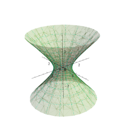
   (A) $K=1$ in $\mathbb{L}^{3}$

   

   

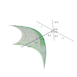
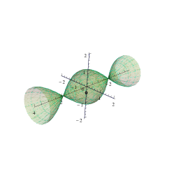
   (B) $K=1$ in $\mathbb{R}^{3}_{2}$

   Figure 1: Constant Gaussian Curvature $1$

3. $K=-1$:

   • ${\rm d}s^{2}=-{\rm d}u^{2}+\cos^{2}u\,{\rm d}v^{2}$.

     1. ${\bf x}\colon\Big{]}-\frac{\pi}{2},\frac{\pi}{2}\Big{[}\times\mathbb{R}\to\mathbb{L}^{3}$,

        $${\bf x}(u,v)=\left(\cos u\cos v,\cos u\sin v,\int_{0}^{u}\sqrt{1+\sin^{2}t}\,{\rm d}t\right).$$

     2. ${\bf x}\colon\mathbb{R}^{2}\to\mathbb{H}^{2}_{1}\subseteq\mathbb{R}^{3}_{2}$,

        $${\bf x}(u,v)=(\cos u\sinh v,\cos u\cosh v,\sin u).$$

     The same situation in remark 5.1 holds in this case.

   • ${\rm d}s^{2}={\rm d}\tau^{2}-\cosh^{2}\tau\,{\rm d}\vartheta^{2}$.

     1. ${\bf x}\colon\cosh^{-1}\big{(}]1,\sqrt{2}[\big{)}\times\mathbb{R}\to\mathbb{L}^{3}$,

        $${\bf x}(\tau,\vartheta)=\left(\int_{0}^{\tau}\sqrt{2-\cosh^{2}t}\,{\rm d}t,\cosh\tau\cosh\vartheta,\cosh\tau\sinh\vartheta\right).$$

     2. ${\bf x}\colon\mathbb{R}^{2}\to\mathbb{H}^{2}_{1}\subseteq\mathbb{R}^{3}_{2}$,

        $${\bf x}(\tau,\vartheta)=(\sinh\tau,\cosh\tau\cos\vartheta,\cosh\tau\sin\vartheta).$$

   If $K=-1$ the surface can be seen, for example, as a piece of one of the following surfaces (again up to isometries of the ambient):

   

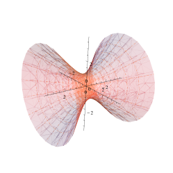
   (A) $K=-1$ in $\mathbb{R}^{3}_{2}$

   

   

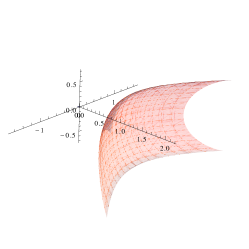
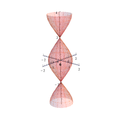
   (B) $K=-1$ in $\mathbb{L}^{3}$

   Figure 2: Constant Gaussian Curvature $-1$

   Finally, we note that the surfaces in figure 1LABEL:sub@fig:K1L3 and figure 2LABEL:sub@fig:K-1R32 are isometric when seen as surfaces in $\mathbb{R}^{3}$ (with its induced metric) but in the pseudo-Riemannian ambients considered here they have rotational symmetry around axes with distinct causal types. The same holds for the corresponding surfaces in figures 1LABEL:sub@fig:K1R32 and 2LABEL:sub@fig:K-1L3.

Ivo Terek Couto
Instituto de Matemática e Estatística
Universidade de São Paulo
E-mail address: terek@ime.usp.br

Alexandre Lymberopoulos
Instituto de Matemática e Estatística
Universidade de São Paulo
E-mail address: lymber@ime.usp.br

References

- [1] Rafael López, Surfaces of Constant Gauss Curvature in Lorentz-Minkowski Three-Space, Rocky Mountain J. Math., 33 (2003), 971-993.
- [2] J. A. Aledo, J. M. Espinar, J. A. Gálvez, Timelike Surfaces in the Lorentz-Minkowski Space with Prescribed Gaussian Curvature and Gauss Map, J. Geom. Phys. 56 (2006), 1357-1369.
- [3] C. H. Gu, H. S. Hu, J-I. Inoguchi, On time-like surfaces of positive constant Gaussian curvature and imaginary principal curvatures, J. Geom. Phys. 41 (2002), 296-311.
- [4] Joseph A. Wolf, Spaces of Constant Curvature, sixth edition, AMS Chelsea Publishing, 2011.
- [5] Barret O’Neill , Semi-Riemannian Geometry With Applications to Relativity, Academic Press, 1983.
- [6] Barret O’Neill, The Geometry of Kerr Black Holes, Dover Books on Physics, 2011.
- [7] John Oprea, Differential Geometry and its Applications, The Mathematical Association of America, 2007.
- [8] Christian Bär, Elementary Differential Geometry, Cambridge University Press, 2010.