Intra- and intercycle interference of electron emission in laser assisted XUV atomic ionization
Abstract
We study the ionization of atomic hydrogen in the direction of polarization due to a linearly polarized XUV pulse in the presence a strong field IR. We describe the photoelectron spectra as an interference problem in the time domain. Electron trajectories steming from different optical laser cycles give rise to intercycle interference energy peaks known as sidebands. These sidebands are modulated by a grosser structure coming from the intracycle interference of the two electron trajectories born during the same optical cycle. We make use of a simple semiclassical model which offers the possibility to establish a connection between emission times and the photoelectron kinetic energy. We compare the semiclassical predictions with the continuum-distorted wave strong field approximation and the ab initio solution of the time dependent Schrödinger equation. We analyze such interference pattern as a function of the time delay between the IR and XUV pulse and also as a function of the laser intensity.
pacs:
32.80.Rm, 32.80.Fb, 03.65.SqI Introduction
New sources of coherent XUV and soft-X-ray radiations delivering pulses with durations in the femtosecond range and with unprecedented high intensities open new perspectives in atomic and molecular physics. Such sources produced from either high-order harmonics or from X-ray free-electron laser (XFEL) paves the way to explore the dynamics of atomic, molecular, and even solid-surface systems undergoing inner-shell transitions. In this way, multi-photon spectroscopy involving synchronized IR and XUV pulses in the strong field regime can be achieved. The photoelectron spectra from rare gas atoms have been extensively studied in the simultaneous presence of two pulses from the XUV source and from an IR laser with a time-controlled delay working as a pump-probe experiment Taïeb et al. (1996); Schins et al. (1996).
The two-color multiphoton ionization where one of the two radiation fields has low intensity and relatively high frequency while the other is intense with a low frequency is usually known as laser assisted photoemission (LAPE). Depending on the features of both laser fields (typically the pulse durations), two well-known regimes –streak camera and sideband– can be distinguished Itatani et al. (2002); Frühling et al. (2009); Wickenhauser et al. (2006); Nagele et al. (2011); Düsterer et al. (2013); Kazansky and Kabachnik (2010, 2009). In the former, the XUV pulse is much shorter than the IR period and, therefore, the electron behaves like a classical particle that gets linear momentum from the IR laser field at the instant of ionization Drescher and Krausz (2005). On the other hand, when the XUV pulse is longer than the laser period , the photoelectron energy spectrum shows a main line associated with the absorption of one XUV photon accompanied by sideband lines, located more or less symmetrically on its sides. The equally spaced sidebands, that are separated from each other by , are associated with additional exchange of laser photons of frequency through absorption and stimulated emission processes. The analysis of the resulting two color photoelectron spectra can provide information about the high-frequency pulse duration, laser intensity, and the time delay between the two pulses. However, the intermediate situation the duration of the XUV pulse is comparable to the laser period has not been thoroughly studied.
An accurate theoretical description of the process must be based on quantum mechanical concepts, i.e. by solving ab initio the time dependent Schödinger equation (TDSE) for the atomic system in the presence of the two pulses. However, the precise calculation of the response of a rare gas atom presents considerable difficulties. The numerical resolution of the TDSE for a multi-electron system rely on the single-active electron approximation, with model potentials that permit one to reproduce the bound state spectrum of the atom with a satisfactory accuracy Nandor et al. (1999); Muller (1999), but results are sensitive to the used approximation. Simplified models have been proposed, such as the the Simpleman’s classical model Schins et al. (1994), the soft-photon approximation Maquet and Taíeb (2007); Jiménez-Galán et al. (2013); Taïeb et al. (2008); Kroll and Watson (1973) for large pulse durations case, and the strong field approximation (SFA) and Coulomb-Volkov approximation (CVA) in the streaking to sideband transition regime Kazansky and Kabachnik (2010); Bivona et al. (2010). These models provide a useful description of some general features. At the time of discussing the physical content of the experimental data or full numerical results, it is instructive to compare them to the qualitative predictions of a simplified analysis. In Ref. Arbó et al. (2010a, b), starting from a semiclassical description of above-threshold ionization (ATI) by a one color laser it has been identified the interplay of intracycle and intercycle interferences between trajectories of electrons emitted at different times, giving rise to a description of the photoelectron spectra of direct electrons as the interplay of such inter- and intracycle interference pattern.
In this paper we use a semiclassical approximation Arbó et al. (2010a, b) to analyze the laser assisted electron photoemission spectra of hydrogen atoms by a XUV pulse, particularly in the intermediate case where or few IR cycles. We show that the role of the IR laser field is threefold: (a) due to the average wiggling of the electron it shifts the energy of the continuum states of the atom by the ponderomotive energy , (b) besides the absorption of the high frequency photon, several IR photons can be absorbed or emitted in the course of the ionization process, and (c) it is responsible for modulations in the photoelectron energy spectrum. For (b), we show that the exchange of IR photons in the energy domain can be interpreted as the interference among different electron trajectories emitted by the atom at different optical cycles giving origin to the formation of sidebands. More importantly, for (c), the interfering electron trajectories within the same optical cycle give rise to a well-determined modulation pattern encoding information of the ionization process in the subfemtosecond time scale.
The paper is organized as follows. In Sec. II we describe the different methods of calculating the photoelectron spectra for the case of laser assisted XUV ionization: By solving the TDSE ab initio, making use of the theory of the strong field approximation (SFA), and a semiclassical model which gives rise to simple analytical expressions. In Sec. III, we present the results and discuss over the comparison of results calculated within the different methods. Concluding remarks are presented in Sec. IV. Atomic units are used throughout the paper, except when otherwise stated.
II Theory and methods of laser-assisted photoemission
We want to solve the problem of atomic ionization by an XUV pulse in the presence of an IR laser both linearly polarized along the direction. The time-dependent Schrödinger equation (TDSE) in the single active electron (SAE) approximation reads
| (1) |
where the hamiltonian of the system within the dipole approximation in the length gauge is expressed as
| (2) |
The first term in Eq. (2) corresponds to the active electron kinetic energy, the second term is the potential energy of the active electron due to the Coulomb interaction with the core, and the last two terms correspond to the interaction of the atom with the electric fields and of the XUV pulse and IR laser, respectively.
As a consequence of the interaction, the bound electron in the initial state is emitted with momentum and energy into the final unperturbed state . The photoelectron momentum distributions can be calculated as
| (3) |
where is the T-matrix element corresponding to the transition .
II.1 Time-Dependent Schrödinger Equation
The evolution of the electronic state is governed by the TDSE in Eq. (1) for the Hamiltonian of Eq. (2). In order to numerically solve the TDSE in the dipole approximation for the SAE, we employ the generalized pseudo-spectral method Tong and Chu (1997, 2000); Tong and Lin (2005). This method combines the discretization of the radial coordinate optimized for the Coulomb singularity with quadrature methods to allow stable long-time evolution using a split-operator representation of the time-evolution operator. Both the bound as well as the unbound parts of the wave function can be accurately represented. Due to the cylindrical symmetry of the system the magnetic quantum number is conserved. After the end of the laser pulse the wave function is projected on eigenstates of the free atomic Hamiltonian with positive eigenenergy and orbital quantum number to determine the transition amplitude to reach the final state (see Refs. Schoëller et al. (1986); Messiah (1965); Dionissopoulou et al. (1997)):
| (4) |
In Eq. (4), is the momentum-dependent atomic phase shift, is the angle between the electron momentum and the polarization direction , and is the Legendre polynomial of degree . In order to avoid unphysical reflections of the wave function at the boundary of the system, the length of the computing box was chosen to be 1200 a.u. ( nm) which is much larger than the maximum quiver amplitude a.u. at the intensity of W/cm2 and the wavelength of 750 nm. The maximum angular momentum included was .
II.2 Strong Field Approximation
Within the time-dependent distorted wave theory, the transition amplitude in the prior form and length gauge is expressed as
| (5) |
where is the initial atomic state with ionization potential and is the distorted final state. As the SFA neglects the Coulomb distortion in the final channel, the distorted final wave function can be written as where Wolkow (1935)
| (6) |
is the length-gauge Volkov state and is the vector potential due to the combined electron field
| (7) |
For the sake of simplicity, hereinafter we consider ionization of a hydrogenic atom of nuclear charge
II.3 Semiclassical model
From TDSE and SFA calculations we have observed that the first and second terms in Eq. (5) are well separated in the energy domain: Whereas the single-photon XUV ionization (first term) leads to ionization of electrons with final kinetic energy close to (with the photon energy of the XUV pulse), the ionization due to the IR laser (second term) leads to ionization of electrons with final kinetic mostly less than twice its ponderomotive energy If we focus on the emission due to the XUV pulse around energy the contribution of the second term in Eq. (5) is negligible wether . Therefore, inserting Eq. (6) into Eq. (5), the transition amplitude within the SFA reads
| (8) |
where the dipole element is given by
| (9) |
Let us suppose that the XUV pulse has the form where is a slowly nonzero varying envelope function in the time interval with duration . In this case, writing , the transition amplitude can be written as where and correspond to the absorption and emission of an XUV photon, respectively. We can discard the emission term since it does not lead to ionization. In other words, according to the rotating wave approximation contribution lays in an energy domain close to which is not in the continuum. Therefore, we can write
| (10) |
where
| (11) |
is the generalized action for the case of LAPE for absorption of a single XUV photon. As the frequency of the XUV pulse is much higher than the IR laser frequency, for XUV pulses not much more intense than the IR laser, we can consider the vector potential as due to the laser field only, i.e., neglecting its XUV contribution Picca et al. (2013).
In order to calculate the transition amplitude we need to solve the four-dimensional integral of equations (10 and 9). When the XUV pulse in shorter than the period of the IR laser, i.e., the electron is emitted with kinetic energy that depends of the vector potential at the ionization time, what is known as streak camera Drescher and Krausz (2005); Goulielmakis et al. (2004); Itatani et al. (2002); Meyer et al. (2006); Kazansky and Kabachnik (2010). However, from now on, we restrict to the case where the XUV pulse is comparable to or longer than the period of the IR laser, i.e., Specifically, the SCM consists of solving the time integral of Eq. (10) by means of the saddle point approximation (SPA) Chirilă and Potvliege (2005); Corkum et al. (1994); Ivanov et al. (1995); Lewenstein et al. (1995). In this sense, the transition probability can be written as a coherent superposition of classical trajectories with the same final momentum as
| (12) |
where are the ionization times corresponding to the stationary points of the action, i.e., Then, from Eq. (11), the ionization times fulfill the equation
| (13) |
Let us consider an IR electric field which is a good approximation for long laser pulses where we can neglect the effect of the envelope. The vector potential is, thus, . In the following we restrict our analysis to forward emission in the direction of polarization, i.e., and . Under condition, where is the electron momentum for ionization of an XUV pulse only, there are two ionization times per optical cycle. They are the early ionization time and the late ionization time corresponding to the th optical cycle, with with [see Fig. 1 (b) and (d)]. In order to find the expressions for we must consider two cases: and , with solutions
| (14) | |||||
and
| (15) |
respectively.

Real ionization times are in the framework of classical trajectories of escaping electrons. Eq. (13) delimits the classical realm to momentum values In other words, the possible classical values of the electron momentum along the positive polarization axis are restricted to . Outside this domain, ionization times are complex due to the non-classical nature of such electron trajectories. The imaginary part of these ionization times gives rise to exponentially decaying factors, for what complex (non-classical) trajectories posses minor relevance compared to real (classical) ones. In consequence, hereinafter we restrict our SCM to classical trajectories.
Including Eq. (12) into Eq. (3), The ionization probability is calculated as
| (16) |
with corresponding to the early (late) release times of Eq. (14) [Eq. (15)]. Assuming now that the depletion of the ground-state is negligible, the ionization rate [the prefactor before the exponential in Eq. (16)] is identical for all subsequent ionization bursts (or trajectories) and is only a function of the time-independent final momentum . This is only valid for the special case that the IR laser is a plane wave with no envelope and also the envelope of the XUV pulse is time independent, i.e., flattop pulse, and where the effect of the Coulomb potential on the receding electron is negliglible (SFA). We consider that the flattop XUV pulse comprises an integer number of IR optical cycles, i.e., . As there are two interfering trajectories per optical cycle of the IR field, the total number of interfering trajectories with final momentum is , with being the number of IR cycles involved. The sum over interfering trajectories in Eq. (16) can thus be decomposed into those associated with the two release times within the same cycle and those associated with release times in different cycles. Consequently, the momentum distribution [Eq. (16)] can be written within the SCM as
| (17) |
where the second factor on the right hand side of Eq. (17) describes the interference of the classical trajectories with final momentum , and is a function of through equations (14) and (15) wether and , respectively. The ionization probability is given by
| (18) |
where was defined in Eq. (9).
With a bit of algebra Eq. (17) can be written as
| (19) |
where is the average action of the two trajectories released in the th cycle, and is the accumulated action between the two release times and within the same -th cycle. The two solutions of Eq. (14) [Eq. (15)] per optical cycle: The early release time and the late release time lays within the first (or third) quarter of the -th cycle and within the second (or fourth) quarter of the -th cycle, respectively.
From Eq. (11), the semi-classical action along one electron trajectory with ionization time is, up to a constant,
| (20) |
The average action depends linearly on the cycle number ,
| (21) |
where is a constant which will be cancelled out when taken the absolute value in Eq. (17), and .
On the other hand, the difference of the action is a constant independent of the cycle number , which can be expressed (dropping out the subindex ) as
| (22) | |||||
where denotes the sign function. We note there is a discontinuity of for . This occurs in the present case where the XUV pulse starts at the same time that . In general, the discontinuity of depends on the delay between both pulses. In the next section we show how this discontinuity mirrors on the electron emission spectra.
In the same way (after some algebra) as for the case of ionization by a monochromatic pulse Arbó et al. (2008, 2010a, 2010b); Xie et al. (2012), Eq. (17) together with equations (19) and (21) can be rewritten as
| (23) |
Eq. (23) indicates that the interference pattern can be factorized in two contributions: (i) the interference stemming from a pair of trajectories within the same cycle (intracycle interference), governed by the factor and (ii) the interference stemming from trajectories released at different cycles (intercycle interference) resulting in the well-known side bands (SBs) given by the factor . When the second factor becomes a series of delta functions, i.e., where
| (24) |
are the positions of the SBs for the absorption of IR photons and one XUV photon. When the emission of IR photons is meant, whereas when the ATI peak for the absorption of only one XUV photon of frequency is described. It is worth to notice that the energy of this ATI peak and the side bands are shifted with the ponderomotive energy of the IR laser according to Eq. (24). The intracycle interference arises from the superposition of pairs of classical trajectories separated by a time slit of the order of less than half a period of the IR laser pulse, i.e., giving access to emission time resolution of fs (for near IR pulses), while the difference between and is , i.e., the optical period of the IR laser. Equation (23) is structurally equivalent to the intensity for crystal diffraction: The factor represents the form (or structure) factor accounting for interference modulations due to the internal structure within the unit cell while the factor gives rise to Bragg peaks due to the periodicity of the crystals. The number of slits is determined by the duration of the XUV pulse Therefore, in Eq. (23) may be viewed as a diffraction grating in the time domain consisting of slits with being the diffraction factor for each slit. As in each optical cycle there are two interfering electron trajectories, it is reasonable to obtain a young-type intracycle interference pattern of the form
III Results and discussion
In order to compare the different methods described in the last section and probe the general conclusion of the SCM that the momentum distribution can be thought as the interplay between the inter- and intracycle interference processes, we consider flattop envelopes for both the IR and XUV pulses. In this sense, the IR laser field can be written as
| (25) |
where the envelope is given by
| (26) |
and zero otherwise so that the IR laser field is a cosine-like pulse centered in the middle of the pulse, i.e., where is the laser pulse duration comprising an integer number of optical cycles with a central flattop region and linear one-cycle ramp on and ramp off.
In the same way, we can define the XUV pulse as
| (27) |
where the main frequency of the XUV pulse is and we choose the envelope as
| (28) |
and zero otherwise. We consider that there is an integer number of optical cycles into the XUV pulse, i.e., is integer, with linear one-cycle ramp on and ramp off. The time characterizes the delay between the centers of the IR and XUV pulses, and and denotes the beginning and the end of the XUV pulse, respectively.
In Fig. 1 (a) and (c) the total electric field is plotted as a function of time [as defined in equations (7-28)] with IR laser parameters and , and XUV pulse parameters and with duration in (a), and in (c). The XUV pulse opens an active window in the time domain for laser assisted XUV ionization marked with a yellow shadow in Fig. 1. The definitions of the IR and XUV pulses are not capricious but they assure a flattop vector potential fulfilling the boundary conditions In Fig. 1 (b) and (d) we show the values of when and , respectively. They look quite the same since for the chosen parameters the amplitude of the vector potential of the IR laser pulse is times higher than the amplitude of the XUV vector potential.
In the following we analyze how the intercycle interference factor and the intracycle interference factor in Eq. (23) within the SCM control the electron spectrum for LAPE. The factor calculated with the electric field described in Fig. 1 (a) is shown in Fig. 2 (a) in blue thin line as equispaced peaks with separation between consecutive peaks equal to the IR laser frequency The peaks of the function agree perfectly with the energies corresponding to the SBs [see Eq. (24)] marked with thin vertical lines. For an arbitrary value of interfering optical cycles , Eq. (23) predicts secondary peaks per optical cycle produced by the interference of optical cycles (slits) in the laser pulse (diffraction grating). In our case, two minima and a secondary peak is observed due to the interference of three optical cycles (). The intracycle structure factor shown in thick red curve displays oscillations with maxima unrelated to the SBs. The positions of these maxima can be calculated with with integer The separation of consecutive maxima of the intracycle factor depends on energy in a nontrivial way. In this case, the separation of the consecutive intracycle maxima is higher close to the classical boundaries a.u. and a.u. than at intermediate energies. There is a discontinuity of the difference of the action as a function of energy (and ) at . According to Eq. (13), ionization times are calculated as the intersection of the horizontal line with the vector potential . When the two ionization times lay in the second half of the optical cycle of the active window [see Fig. 1 (b)]. As approaches the early release time goes to the middle of the active window whereas the late release times goes to the end of it. In turn, when the situation is different: As approaches the early release time goes to the beginning of the active window whereas the late release times goes to the middle. Such discontinuity does not exist in the case of intracycle interference in above threshold ionization by an IR pulse since, in that case, (there is no XUV pulse) in Eq. (22) Arbó et al. (2008, 2010a, 2010b); Xie et al. (2012).
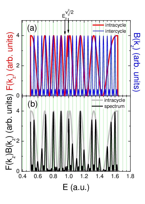
In Fig. 2 (b) we show the interference pattern for the case of interfering cycles into the active window [Fig. 1 (c) and (d)]. Only the factor is displayed setting the variation of the ionization rate to unity to focus on the interference process. For the sake of comparison, in light gray the intracycle pattern of (a) is also displayed. We observe that the intercycle SB peaks given by [Fig. 2 (a)] are modulated by the intracycle interference factor . The intracycle interference can lead to the suppression of SBs (for example, near ).

We need to compare our SCM with quantum SFA and ab initio calculations by solving numerically the TDSE. In Fig. 3 we plot the energy distribution of electron emission in the forward direction for the same laser pulse described in Fig. 1. We perform SFA and TDSE calculations in Fig. 3 (a) and Fig. 3 (b), respectively, for two different durations of the XUV pulse. For the case of we observe a set of peaks separated by the laser frequency in agreement with Eq. (24) whose positions are illustrated with vertical thin lines. By comparing Fig. 2 and Fig. 3, we see that the quantum (TDSE and SFA) energy distributions extend about a.u. beyond the classical limits . The agreement between SFA and TDSE results is remarkable and both are qualitatively similar to the SCM of Fig. 2. We would like to point out that the energy distributions exhibit sharp modulations in agreement with the intracycle interference pattern calculated with an XUV pulse duration in gray thick line. In this sense, the fact that the intracycle interference pattern modulates the sidebands in the energy distribution, albeit derived within the SCM, is also valid for the quantum calculations. The reason for this is under current investigation, however we note that it is in close relationship with previous work Kazansky and Kabachnik (2010); Bivona et al. (2010) where the PE spectra is factorized as two contributions. It is also worth to mention that, as within the SCM, there are frustrated SBs, i.e., close to and coinciding with the minima of the intracycle interference pattern

In order to investigate the dependence of the intracycle interference pattern on the intensity of the laser pulse, we perform calculations of the energy distribution in the forward direction within the SCM in Fig. 4 (a), the SFA in Fig. 4 (b), and the TDSE in Fig. 4 (c) for laser field amplitudes from up to In this sense, the intracycle pattern in Fig. 2 (a) is a cut of Fig. 4 (a) at The same applies to the intracycle patterns of Fig. 3 (a) and (b) with Fig. 4 (b) and (c), respectively. The classical boundaries are drawn in dash lines and they exactly delimit the SCM spectrogram of Fig. 4 (a), as expected. The discontinuity at is clearly independent of the laser field amplitude. Above the discontinuity, the interference maxima (and minima) exhibit a positive slope as a function of whereas below it, the stripes have negative slope. The classical boundaries slightly blur for the SFA spectrogram, also showing the characteristic intracycle stripes with positive (negative) slope close to the top (bottom) classical boundary. For intermediate energies close to it is difficult to determine such discontinuity. In Fig. 4 (c), the TDSE calculation exhibit a strong probability distribution for high values of in the low energy region. The source of this enhancement of the probability is atomic ionization by the IR laser pulse alone, which has not been considered in our SCM and is strongly suppressed in the SFA because the laser photon energy is much less than the ionization potential, i.e., For this reason we can confirm that the SFA is a very reliable method to deal with LAPE rather than ATI by IR lasers. Except for the region where ionization by the laser field alone becomes important, SFA and TDSE spectrograms agree with each other and qualitatively resemble the SCM calculations.

So far, we have performed our analysis of the electron emission in the forward direction for zero time delay, i.e., the center of the IR laser and XUV pulses coincide as In order to reveal how the intracycle interference pattern changes with the time delay, we vary from up to This means that the center of the XUV pulse situated at corresponds to a phase into the laser optical cycle In Fig. 5 (a) we show the SCM intracycle interference pattern in the forward direction as a function of the time delay . The horizontal stripes show the independence of the intracycle interference pattern with the time delay, except for the discontinuity in Eq. (22) for values of energy equal to . For the discontinuity is situated at since as is shown in Fig. 2. As (and ) varies, the discontinuity follows the shape of the vector potential. For the cases that and the discontinuity moves to the classical boundary loosing entity. For the case the separation between consecutive intracycle interference stripes is smaller for lower energies and increases as the energy grows. Contrarily, for energy separation between consecutive intracycle interference maxima is higher for lower energy and diminishes as energy increases. The SFA and TDSE energy distribution in Fig. 5 (b) and (c), respectively, exhibit similar characteristics to the SCM. Interestingly, the discontinuity at can be clearly observed for the same energy values. The resemblance between the SFA and TDSE results is remarkable, which shows that the SFA is a very appropriate method to deal with LAPE processes and computationally much less demanding than solving the TDSE ab initio. Low energy contributions in TDSE calculations [Fig. 5 (c)] are due to ionization by the interaction between the atom and the IR laser pulse alone. There are two characteristics of SFA and TDSE spectra which deserve more study: (i) For the energy distribution extends to lower energy values than for other values , whereas for it extends for higher energy values (), and (ii) the horizontal intracycle interference stripes show some structure at the right of the above mentioned discontinuity, i.e., which is absent at the left of it, i.e., .
When we calculate the energy distribution for a XUV pulse with duration , our active window comprises two IR optical cycles. For the particular case of zero time delay, i.e., (both IR and XUV pulses centered at the same instant of time), the vector potential at the beginning of the active window has a change of sign compared to the case. Therefore, for the sake of comparison, we redefine the phase varying the time delay from up to In this sense, with this new definition, corresponds to with the same behavior of the vector potential inside the active window. In Fig. 5 (d) the SCM spectrum display horizontal lines corresponding to the intercycle interference, which are modulated by the intracycle pattern of Fig. 5 (a). The discontinuity of the intracycle modulation can also be observed, which stands for the SFA [Fig. 5 (e)] and TDSE [Fig. 5 (f)] too. Once again, the agreement between the SFA and TDSE is very good, with the exception of the low energy contribution due to the ionization by the IR laser pulse in the TDSE spectrogram. By comparing the intracycle pattern for on the left column [Figs. 5 (a), (b), and (c)] to the whole interference pattern for on the right column [Figs. 5 (d), (e), and (f)], we see the interplay between intra- and intercycle interference, i.e., the intracycle interference pattern works as a modulation of the intercycle interference pattern (SBs) for the active window with duration of two optical laser cycles.

The intracycle energy distributions () in Fig. 2, Fig. 3 (a), and Fig. 3 (b) can be regarded as cuts of the intracycle interferograms of Figs. 5 (a), (b), and (c), respectively. For the sake of completeness, we show also in the left column of Fig. 6 [(a), (b), and (c)] the energy distribution for for and We observe how in all calculations [SCM in Fig. 6 (a), SFA in Fig. 6 (b), and TDSE in Fig. 6 (c)] the separation of consecutive intracycle maximum grows as the energy increases. The energy distributions for show a SB structure (intercycle interference) modulated by the intracycle interference pattern. As the separation of intracycle maxima of the intracycle interference pattern near the lower classical limit is close to the laser photon energy , it competes with the intercycle interference pattern (SBs) for whose separation is also Therefore, the interplay of intra- and intercycle interference pattern gives rise to new oscillation structures of the energy distribution by ionization of the XUV pulse of duration assisted by the laser pulse. For example, a gross structure is observed Fig. 6 (b) and (c) with a minimum at for the SFA and TDSE. The same is valid for the phase in Figs. 6 (d), (e), and (f) for the SCM, SFA, and TDSE, respectively. However, in this case, the competition between intra- and intercycle interference patterns takes place close to the higher classical limit. Again, a grosser structure is formed making the energy distributions when for and to be similar. It is expected that as the active window gets wider, i.e., the agreement between energy spectra for and improves.
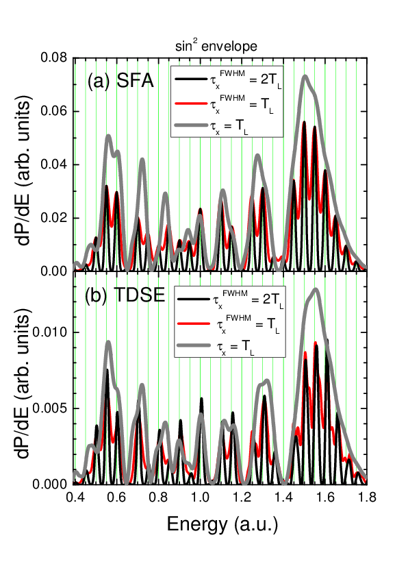
In the following we investigate the role of the envelope of the XUV pulse on LAPE. So far, we have used the trapezoidal envelope given by Eq. (28), which opens a well-defined active window of duration almost equal to (since it has a one-cycle ramp on and one-cycle ramp off of duration each). Now, we consider an XUV pulse with squared sine envelope
| (29) |
where is the FWHM duration of the electric field. The result for the energy distribution in the forward direction due to an XUV pulse with envelope with assisted by the laser pulse described in equations (25) and (26) shows modulated SB peaks Fig. 7 (a) and (b) calculated within the SFA and TDSE, respectively. When we compare these results with the energy distribution calculated with the flattop pulse of equations (27) and (28), we realize that the origin of the modulations of the SBs are due to the intracycle interference also for the XUV envelope of Eq. (29). When we double the duration of the XUV pulse, i.e., , the SB peaks are sharper because the double of the optical cycles are involved in the active window enhancing, consequently, the intercycle interference giving rise to almost perfect destructive interference (minima of the energy distribution are zero). The agreement between SFA and TDSE calculations is very good. We can say, therefore, that the envelope of the XUV pulse play a minor role in LAPE and most of the conclusions derived for the flattop XUV pulse are still valid for a smooth experimental-like envelope shape.
IV Conclusions
We have studied the electron emission in the forward direction produced by hydrogen ionization subject to a XUV and laser pulse both linearly polarized in the same direction. The PE spectrum can be regarded as an interference pattern of a diffraction grating in the time domain. Semiclassically, the intercycle interference of electron trajectories from different optical cycles gives rise to side bands, whereas the intracycle interference of electron trajectories born in the same optical cycle originates a coarse grained pattern modulating the side bands. We have observed that the SFA is sufficiently accurate to describe the photoelectron spectrum when compared to the TDSE. The intracycle pattern is independent of the XUV pulse duration and envelope but exhibits a jump at a given energy as a function of the time delay between the two pulses reproducing the profile of the laser vector potential.
Acknowledgements.
Work supported by CONICET PIP0386, PICT-2012-3004 and PICT-2014-2363 of ANPCyT (Argentina), and the University of Buenos Aires (UBACyT 20020130100617BA). Work triggered by discussion between Pablo Macri and D.G.A.References
- Taïeb et al. (1996) R. Taïeb, V. Véniard, and A. Maquet, J. Opt. Soc. Am. B 13, 363 (1996).
- Schins et al. (1996) J. M. Schins, P. Breger, P. Agostini, R. C. Constantinescu, H. G. Muller, A. Bouhal, G. Grillon, A. Antonetti, and A. Mysyrowicz, J. Opt. Soc. Am. B 13, 197 (1996).
- Itatani et al. (2002) J. Itatani, F. Quéré, G. L. Yudin, M. Y. Ivanov, F. Krausz, and P. B. Corkum, Phys. Rev. Lett. 88, 173903 (2002).
- Frühling et al. (2009) U. Frühling, M. Wieland, M. Gensch, T. Gebert, B. Schutte, M. Krikunova, R. Kalms, F. Budzyn, O. Grimm, J. Rossbach, E. Plonjes, and M. Drescher, Nat Photon 3, 523 (2009).
- Wickenhauser et al. (2006) M. Wickenhauser, J. Burgdörfer, F. Krausz, and M. Drescher, Journal of Modern Optics 53, 247 (2006), http://dx.doi.org/10.1080/09500340500259870 .
- Nagele et al. (2011) S. Nagele, R. Pazourek, J. Feist, K. Doblhoff-Dier, C. Lemell, K. Tőkési, and J. Burgdörfer, Journal of Physics B: Atomic, Molecular and Optical Physics 44, 081001 (2011).
- Düsterer et al. (2013) S. Düsterer, L. Rading, P. Johnsson, A. Rouzée, A. Hundertmark, M. J. J. Vrakking, P. Radcliffe, M. Meyer, A. K. Kazansky, and N. M. Kabachnik, Journal of Physics B: Atomic, Molecular and Optical Physics 46, 164026 (2013).
- Kazansky and Kabachnik (2010) A. K. Kazansky and N. M. Kabachnik, Journal of Physics B: Atomic, Molecular and Optical Physics 43, 035601 (2010).
- Kazansky and Kabachnik (2009) A. K. Kazansky and N. M. Kabachnik, Journal of Physics B: Atomic, Molecular and Optical Physics 42, 121002 (2009).
- Drescher and Krausz (2005) M. Drescher and F. Krausz, Journal of Physics B: Atomic, Molecular and Optical Physics 38, S727 (2005).
- Nandor et al. (1999) M. J. Nandor, M. A. Walker, L. D. Van Woerkom, and H. G. Muller, Phys. Rev. A 60, R1771 (1999).
- Muller (1999) H. G. Muller, Phys. Rev. A 60, 1341 (1999).
- Schins et al. (1994) J. M. Schins, P. Breger, P. Agostini, R. C. Constantinescu, H. G. Muller, G. Grillon, A. Antonetti, and A. Mysyrowicz, Phys. Rev. Lett. 73, 2180 (1994).
- Maquet and Taíeb (2007) A. Maquet and R. Taíeb, Journal of Modern Optics 54, 1847 (2007), http://dx.doi.org/10.1080/09500340701306751 .
- Jiménez-Galán et al. (2013) A. Jiménez-Galán, L. Argenti, and F. Martín, New Journal of Physics 15, 113009 (2013).
- Taïeb et al. (2008) R. Taïeb, A. Maquet, and M. Meyer, Journal of Physics: Conference Series 141, 012017 (2008).
- Kroll and Watson (1973) N. M. Kroll and K. M. Watson, Phys. Rev. A 8, 804 (1973).
- Bivona et al. (2010) S. Bivona, G. Bonanno, R. Burlon, and C. Leone, Laser Physics 20, 2036 (2010).
- Arbó et al. (2010a) D. G. Arbó, K. L. Ishikawa, K. Schiessl, E. Persson, and J. Burgdörfer, Phys. Rev. A 81, 021403 (2010a).
- Arbó et al. (2010b) D. G. Arbó, K. L. Ishikawa, K. Schiessl, E. Persson, and J. Burgdörfer, Phys. Rev. A 82, 043426 (2010b).
- Tong and Chu (1997) X. M. Tong and S. I. Chu, Chem. Phys. 217, 119 (1997).
- Tong and Chu (2000) X.-M. Tong and S.-I. Chu, Phys. Rev. A 61, 031401 (2000).
- Tong and Lin (2005) X. M. Tong and C. D. Lin, Journal of Physics B: Atomic, Molecular and Optical Physics 38, 2593 (2005).
- Schoëller et al. (1986) O. Schoëller, J. S. Briggs, and R. M. Dreizler, Journal of Physics B: Atomic and Molecular Physics 19, 2505 (1986).
- Messiah (1965) A. Messiah, (1965), north-Holland, New York.
- Dionissopoulou et al. (1997) S. Dionissopoulou, T. Mercouris, A. Lyras, and C. A. Nicolaides, Phys. Rev. A 55, 4397 (1997).
- Wolkow (1935) D. Wolkow, Zeitschrift für Physik 94, 250 (1935).
- Picca et al. (2013) R. D. Picca, J. Fiol, and P. D. Fainstein, Journal of Physics B: Atomic, Molecular and Optical Physics 46, 175603 (2013).
- Goulielmakis et al. (2004) E. Goulielmakis, M. Uiberacker, R. Kienberger, A. Baltuska, V. Yakovlev, A. Scrinzi, T. Westerwalbesloh, U. Kleineberg, U. Heinzmann, M. Drescher, and F. Krausz, Science 305, 1267 (2004), http://science.sciencemag.org/content/305/5688/1267.full.pdf .
- Meyer et al. (2006) M. Meyer, D. Cubaynes, P. O’Keeffe, H. Luna, P. Yeates, E. T. Kennedy, J. T. Costello, P. Orr, R. Taïeb, A. Maquet, S. Düsterer, P. Radcliffe, H. Redlin, A. Azima, E. Plönjes, and J. Feldhaus, Phys. Rev. A 74, 011401 (2006).
- Chirilă and Potvliege (2005) C. C. Chirilă and R. M. Potvliege, Phys. Rev. A 71, 021402 (2005).
- Corkum et al. (1994) P. B. Corkum, N. H. Burnett, and M. Y. Ivanov, Opt. Lett. 19, 1870 (1994).
- Ivanov et al. (1995) M. Ivanov, P. B. Corkum, T. Zuo, and A. Bandrauk, Phys. Rev. Lett. 74, 2933 (1995).
- Lewenstein et al. (1995) M. Lewenstein, K. C. Kulander, K. J. Schafer, and P. H. Bucksbaum, Phys. Rev. A 51, 1495 (1995).
- Arbó et al. (2008) D. G. Arbó, K. I. Dimitriou, E. Persson, and J. Burgdörfer, Phys. Rev. A 78, 013406 (2008).
- Xie et al. (2012) X. Xie, S. Roither, D. Kartashov, E. Persson, D. G. Arbó, L. Zhang, S. Gräfe, M. S. Schöffler, J. Burgdörfer, A. Baltuška, and M. Kitzler, Phys. Rev. Lett. 108, 193004 (2012).
- Smirnova et al. (2003) O. Smirnova, V. S. Yakovlev, and A. Scrinzi, Phys. Rev. Lett. 91, 253001 (2003).
- Johnsson et al. (2005) P. Johnsson, R. López-Martens, S. Kazamias, J. Mauritsson, C. Valentin, T. Remetter, K. Varjú, M. B. Gaarde, Y. Mairesse, H. Wabnitz, P. Salières, P. Balcou, K. J. Schafer, and A. L’Huillier, Phys. Rev. Lett. 95, 013001 (2005).
- Schütte et al. (2012) B. Schütte, S. Bauch, U. Frühling, M. Wieland, M. Gensch, E. Plönjes, T. Gaumnitz, A. Azima, M. Bonitz, and M. Drescher, Phys. Rev. Lett. 108, 253003 (2012).
- Mauritsson et al. (2008) J. Mauritsson, P. Johnsson, E. Mansten, M. Swoboda, T. Ruchon, A. L’Huillier, and K. J. Schafer, Phys. Rev. Lett. 100, 073003 (2008).
- Johnsson et al. (2007) P. Johnsson, J. Mauritsson, T. Remetter, A. L’Huillier, and K. J. Schafer, Phys. Rev. Lett. 99, 233001 (2007).
- Kazansky et al. (2009) A. K. Kazansky, I. P. Sazhina, and N. M. Kabachnik, Journal of Physics B: Atomic, Molecular and Optical Physics 42, 245601 (2009).
- Cao et al. (2008) W. Cao, P. Lu, P. Lan, Y. Li, and X. Wang, Journal of Physics B: Atomic, Molecular and Optical Physics 41, 085601 (2008).
- Kazansky and Kabachnik (2007a) A. K. Kazansky and N. M. Kabachnik, Journal of Physics B: Atomic, Molecular and Optical Physics 40, F299 (2007a).
- Kazansky and Kabachnik (2007b) A. K. Kazansky and N. M. Kabachnik, Journal of Physics B: Atomic, Molecular and Optical Physics 40, 2163 (2007b).
- Kazansky and Kabachnik (2007c) A. K. Kazansky and N. M. Kabachnik, Journal of Physics B: Atomic, Molecular and Optical Physics 40, 3413 (2007c).
- Kazansky and Kabachnik (2006) A. K. Kazansky and N. M. Kabachnik, Journal of Physics B: Atomic, Molecular and Optical Physics 39, 5173 (2006).
- Kazansky et al. (2013) A. K. Kazansky, I. P. Sazhina, and N. M. Kabachnik, Journal of Physics B: Atomic, Molecular and Optical Physics 46, 025601 (2013).
- Uiberacker et al. (2007) M. Uiberacker, T. Uphues, M. Schultze, A. J. Verhoef, V. Yakovlev, M. F. Kling, J. Rauschenberger, N. M. Kabachnik, H. Schroder, M. Lezius, K. L. Kompa, H.-G. Muller, M. J. J. Vrakking, S. Hendel, U. Kleineberg, U. Heinzmann, M. Drescher, and F. Krausz, Nature 446, 627 (2007).
- Cavalieri et al. (2007) A. L. Cavalieri, N. Muller, T. Uphues, V. S. Yakovlev, A. Baltuska, B. Horvath, B. Schmidt, L. Blumel, R. Holzwarth, S. Hendel, M. Drescher, U. Kleineberg, P. M. Echenique, R. Kienberger, F. Krausz, and U. Heinzmann, Nature 449, 1029 (2007).
- Drescher et al. (2001) M. Drescher, M. Hentschel, R. Kienberger, G. Tempea, C. Spielmann, G. A. Reider, P. B. Corkum, and F. Krausz, Science 291, 1923 (2001), http://science.sciencemag.org/content/291/5510/1923.full.pdf .
- Goulielmakis et al. (2007) E. Goulielmakis, V. S. Yakovlev, A. L. Cavalieri, M. Uiberacker, V. Pervak, A. Apolonski, R. Kienberger, U. Kleineberg, and F. Krausz, Science 317, 769 (2007), http://science.sciencemag.org/content/317/5839/769.full.pdf .
- Kienberger et al. (2002) R. Kienberger, M. Hentschel, M. Uiberacker, C. Spielmann, M. Kitzler, A. Scrinzi, M. Wieland, T. Westerwalbesloh, U. Kleineberg, U. Heinzmann, M. Drescher, and F. Krausz, Science 297, 1144 (2002), http://science.sciencemag.org/content/297/5584/1144.full.pdf .
- Ben-Hai et al. (2011) Y. Ben-Hai, Z. Dong-Ling, and T. Qing-Bin, Chinese Physics B 20, 83201 (2011).
- Gordon (1926) W. Gordon, Zeitschrift für Physik 40, 117 (1926).
- Picard et al. (2014) Y. J. Picard, B. Manschwetus, M. Géléoc, M. Böttcher, E. M. S. Casagrande, N. Lin, T. Ruchon, B. Carré, J.-F. Hergott, F. Lepetit, R. Taïeb, A. Maquet, and A. Huetz, Phys. Rev. A 89, 031401 (2014).
- Arbó et al. (2014) D. G. Arbó, S. Nagele, X.-M. Tong, X. Xie, M. Kitzler, and J. Burgdörfer, Phys. Rev. A 89, 043414 (2014).
- Arbó et al. (2006a) D. G. Arbó, S. Yoshida, E. Persson, K. I. Dimitriou, and J. Burgdörfer, Phys. Rev. Lett. 96, 143003 (2006a).
- Arbó et al. (2006b) D. G. Arbó, E. Persson, and J. Burgdörfer, Phys. Rev. A 74, 063407 (2006b).
- Véniard et al. (1995) V. Véniard, R. Taïeb, and A. Maquet, Phys. Rev. Lett. 74, 4161 (1995).
- Véniard et al. (1996) V. Véniard, R. Taïeb, and A. Maquet, Phys. Rev. A 54, 721 (1996).
- Yudin et al. (2007) G. L. Yudin, S. Patchkovskii, P. B. Corkum, and A. D. Bandrauk, Journal of Physics B: Atomic, Molecular and Optical Physics 40, F93 (2007).
- Lindner et al. (2005) F. Lindner, M. G. Schätzel, H. Walther, A. Baltuška, E. Goulielmakis, F. Krausz, D. B. Milošević, D. Bauer, W. Becker, and G. G. Paulus, Phys. Rev. Lett. 95, 040401 (2005).
- Hentschel et al. (2001) M. Hentschel, R. Kienberger, C. Spielmann, G. A. Reider, N. Milosevic, T. Brabec, P. Corkum, U. Heinzmann, M. Drescher, and F. Krausz, Nature 414, 509 (2001).
- Bauer and Koval (2006) D. Bauer and P. Koval, Computer Physics Communications 174, 396 (2006).