Topological phase transitions and universality in the Haldane-Hubbard model

Abstract

We study the Haldane-Hubbard model by exact Renormalization Group techniques. We analytically construct the topological phase diagram, for weak interactions. We predict that many-body interactions induce a shift of the transition line: in particular, repulsive interactions enlarge the topologically non-trivial region. The presence of new intermediate phases, absent in the non interacting case, is rigorously excluded at weak coupling. Despite the non-trivial renormalization of the wave function and of the Fermi velocity, the conductivity is universal: at the renormalized critical line, both the discontinuity of the transverse conductivity and the longitudinal conductivity are independent of the interaction, thanks to remarkable cancellations due to lattice Ward Identities. In contrast to the quantization of the transverse conductivity, the universality of the longitudinal conductivity cannot be explained via topological arguments.

I Introduction

The current understanding of topological matter K ; K1 ; K2 is mostly based on a single-particle description. A paradigmatic example is the integer quantum Hall effect: in the absence of interactions, the Hall conductivity has a deep topological interpretationASS ; ASS1 , which explains its quantization and stability. A more recent example is provided by the classification of time-reversal invariant insulators KM ; KM1 ; KM2 ; KM3 ; KM4 ; KM5 ; KM6 ; KM7 , which, again, relies on the properties of the noninteracting Bloch functions. Understanding the effect of interactions on topological matter has become a very active area of research H0 .

A natural model in which to explore such issues is the Haldane-Hubbard model. The Haldane-Hubbard model describes spin-1/2 electrons on the honeycomb lattice, interacting via a local Hubbard interaction of strength $U$. The electrons hop between nearest neighbor sites with hopping strength $t_{1}$, and between next-to-nearest neighbor sites with alternating hopping parameters $t_{2}e^{\pm i\phi}$: the phases $\pm\phi$ describe a transverse magnetic field, with zero net flux through the honeycomb plaquette. Finally, the system is also exposed to a staggered chemical potential, with strength $\pm W$ on the two triangular sublattices. In the absence of interactions H this model shows, depending on the value of its parameters, a trivial insulating phase with vanishing transverse conductivity $\sigma_{12}=0$, or a quantum Hall phase with $\sigma_{12}=\pm 2\frac{e^{2}}{h}$. These topological phases are separated by two critical curves in the $(\phi,W)$ plane, intersecting at the crossing points $(0,0)$ and $(\pi,0)$. Along the critical curves, the energy bands touch at a conical intersection; at the crossing points, there are two such conical intersections, as in standard graphene. Indeed if $t_{2}=W=0$ the system describes graphene with short range interaction.

From a theoretical viewpoint, the Haldane topological phases have been argued to emerge in pure graphene sheets by spontaneous mass generation, due to the strong, unscreened Coulomb repulsion H1 ; H11 ; H12 ; H13 ; H14 ; H15 ; H16 ; GMPgauge . From an experimental viewpoint, the Haldane model has been realized in Ref.E , and the topological phase transition has been observed. The inclusion of a tunable Hubbard interaction seems to be accessible by the present technology. Therefore, studying its effects on the transport coefficients is of fundamental importance for the next generation of cold atom experiments. So far, the properties of the Haldane-Hubbard model have been investigated mostly via mean-field, variational and numerical analysesH3 ; H31 ; H32 ; H33 ; H34 ; H35 ; H36 ; H37 ; H38 ; H39 ; H310 ; H311 ; H312 ; Van ; Hub .

Concerning the transverse conductivity, topological arguments for interacting systemsAS ; HM ensure that, away from the critical curves, $\sigma_{12}$ can only take integer values, in units of $e^{2}/h$ (here $\sigma_{ij}$ are the elements of the conductivity matrix, in the limit of zero frequency and zero temperature). However, its specific value at a given point in the phase diagram can be different from the corresponding non-interacting value, in particular in the vicinity of the critical curves (at weak coupling, far from the critical lines, the conductivity is known to be independent of the interaction CH ; GMPhall ). The relevant question here is to distinguish between two scenarios: the first, in which small interactions are not able to generate new phases and their main effect is a shift of the critical curves, as found in certain 3D topological insulators E2 ; E21 ; E22 ; and a second one, characterized by the emergence of a novel, interaction-induced, topological phase, like the one corresponding to $\sigma_{12}=\pm\frac{e^{2}}{h}$, predicted for the Haldane-Hubbard model in Ref.H3 ; H31 ; H32 ; H33 ; Van ; Hub . Regarding the longitudinal conductivity, in the absence of interactions it is equal to $\frac{e^{2}}{h}\frac{\pi}{4}$, for all the values of $(\phi,W)$ on the critical lines, with the exception of the crossing points $(\phi,W)=(0,0),(\pi,0)$, where it is equal to $\frac{e^{2}}{h}\frac{\pi}{2}$ (of course, away from the critical lines $\sigma_{ii}=0$). There are no topological arguments ensuring that the critical longitudinal conductivity should remain quantized when the interaction is switched on: therefore, the relevant question here is whether the interaction introduces corrections breaking this exact quantization or not. This question is related to a similar one discussed in the context of graphene, in which recent experiments Nair showed that the optical longitudinal conductivity is essentially universal, and in excellent agreement with the value computed for the non-interacting model SPG ; on the contrary, the interaction produces dramatic effects on other physical quantities, such as the Fermi velocity Elias . On the theoretical side, the universal behavior in graphene is still not completely understood L1 ; L11 ; L12 ; L13 ; L14 ; L15 ; L16 ; L17 ; L18 ; L19 , see, in particular, Ref.L17 for a recent review. A rigorous result for short range interaction GMP showed that, in order to get exact universality of graphene’s longitudinal conductivity, one needs to fully take into account the non linear correction to the bands, even if such terms are irrelevant in the Renormalization Group (RG) sense.

In this paper we compute the conductivity matrix of the Haldane-Hubbard model via exact RG methods, close to and at the critical lines, for weak interactions. We take lattice effects into account, and we exploit lattice symmetries in order to reduce the number of independent running couplings, in a way similar to Ref.GM ; GMP ; FA ; HJR for graphene. The use of exact RG methods is motivated by the fact that the computation of conductivity is extremely sensitive to the choice of the regularization schemeL19 . Even though they are irrelevant in the RG sense, lattice and interaction effects produce, in general, finite corrections to the physical observables, and they must be taken into account in order to prove or disprove the emergence of new interaction-induced topological phases, as well as to address the issue of universality of the critical longitudinal conductivity.

By choosing the chemical potential $\mu\equiv\mu(U)$ so to fix the Fermi energy half-way between the valence and conduction bands, the band gap can only close at the two Fermi points $\vec{p}_{F}^{\,\omega}=(\frac{2\pi}{3},\omega\frac{2\pi}{3\sqrt{3}})$, where $\omega=\pm$ is the valley index. We prove that, close to criticality, the interacting Euclidean two-point function is:

$$\hat{S}_{2}(k_{0},\vec{p}_{F}^{\,\omega}+\vec{k}^{\prime})=$$

$$=-\begin{pmatrix}ik_{0}Z_{1,R}-m_{R}&v_{R}(-ik_{1}^{\prime}+\omega k_{2}^{\prime})\\ v_{R}(ik_{1}^{\prime}+\omega k_{2}^{\prime})&ik_{0}Z_{2,R}+m_{R}\end{pmatrix}^{-1}\hskip-2.84544pt\big{(}1+R(k_{0},\vec{k}^{\prime})\big{)}$$

where the error term $R(k_{0},\vec{k}^{\prime})$ is subleading in the effective mass $m_{R}$, in the Matsubara frequency $k_{0}$ and in the quasi-momentum $\vec{k}^{\prime}$. The parameters $Z_{1,R},Z_{2,R},v_{R},m_{R}$, depend non-trivially on the valley index $\omega$ and on the interaction. In particular, the renormalized mass $m_{R}\equiv m_{R,\omega}$ reads:

$$m_{R,\pm}=W\pm 3\sqrt{3}\,t_{2}\sin\phi-F_{\pm}(U,W,\phi)$$ (1)

where $\pm$ is the valley index, and $F_{\pm}$ is expressed in the form of a convergent renormalized series, whose first non-trivial order is given by Eq.(71) below. The dressed critical lines, defined by the condition that the renormalized mass vanishes, are also modified by the interaction, see Fig.1. Similarly, the Fermi velocity $v_{R}$ and the wave function renormalizations $Z_{1,R},Z_{2,R}$ have non-trivial interaction corrections and, remarkably, $Z_{1,R}$ and $Z_{2,R}$ are different, as shown in Fig.2. All these non-universal renormalizations are absent in effective relativistic descriptions: by neglecting the (irrelevant) non-linear corrections to the energy bands, one would obtain a Nambu-Jona Lasinio model, in which Lorentz and chiral symmetry would imply the invariance of $v_{R}$, the invariance of the critical lines and $Z_{1,R}=Z_{2,R}$. However, these extra symmetries are broken by the lattice, and the renormalization of the effective parameters is a physical signature of many body interaction that should be visible in real systems, e.g., in cold atom experiments. These non-universal parameters also enter the computation of the conductivity: remarkably, they are related by exact lattice Ward identities, which induce non-trivial cancellations and imply subtle universality properties, as stated in the following theorem. We recall that $\sigma_{ij}$ are the elements of the Kubo conductivity matrix, in the limit of zero frequency and zero temperature. We also denote by $\sigma_{ij}^{cr}$ their values on the renormalized critical curves.

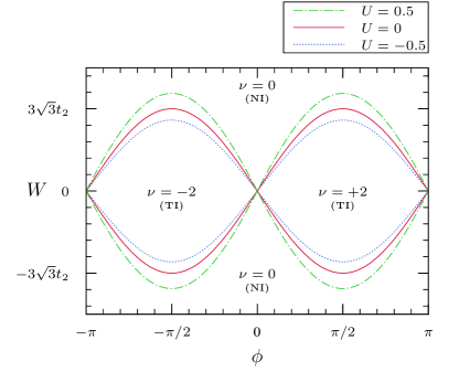
Figure 1: Interacting phase diagram of the Haldane-Hubbard model for $t_{1}=1$, $t_{2}=0.1$, and different values of $U$. $\sigma_{12}=(e^{2}/h)\nu$, where the values of $\nu$ are reported in the figure. for $\nu=\pm 2$ the system is a topological insulator (TI), while for $\nu=0$ the system is a trivial, normal, insulator (NI).

Theorem. There exists $U_{0}>0$ such that for $-U_{0}<U<U_{0}$, the system is massless if and only if the right side of Eq.(1) vanishes. This condition defines two renormalized critical curves intersecting at $(\phi,W)=(0,0),(\pi,0)$, separating two non-trivial topological phases, characterized by transverse conductivity $\sigma_{12}=\pm 2(e^{2}/h)$, from two standard insulating phases, see Fig.1. On the renormalized critical curves, the critical longitudinal conductivity $\sigma_{ii}^{cr}$, $i=1,2$, is quantized: if $\phi\neq 0,\pi$,

$$\sigma_{ii}^{\text{cr}}=\frac{e^{2}}{h}\frac{\pi}{4}\;,$$ (2)

while $\sigma_{ii}^{\text{cr}}=\frac{e^{2}}{h}\frac{\pi}{2}$ at $(\phi,W)=(0,0),(\pi,0)$.

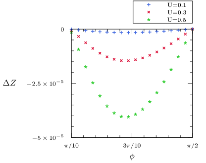
Figure 2: The difference of the wave function renormalizations $\Delta Z=Z_{1,R}-Z_{2,R}$ on the critical line, as a function of $\phi$, for different values of $U$. This difference would be zero for the effective relativistic theory.

Thus, the critical lines acquire non-universal, interaction-dependent corrections, but they still separate topological regions labelled by $\nu=\pm 2$ from the trivial ones, labelled by $\nu=0$, see Fig.1. New intermediate phases characterized by the quantum number $\nu=\pm 1$ are rigorously excluded at weak coupling: the universality class of the topological transition remains unchanged. The effect of the repulsive interaction is to enlarge the topologically non-trivial region, see Fig.1. This enhancement agrees with the numerical findings of Ref.Van ; Hub and is presumably a sign that repulsive interactions in graphene-like systems can favor the spontaneous generation of the topological insulating phase H1 ; H11 ; H12 ; H13 ; H14 ; H15 ; H16 ; GMPgauge .

Even if not protected by any topological argument, the critical longitudinal conductivity $\sigma_{11}^{\text{cr}}$ is exactly universal and equal to half the one of graphene, on the whole critical line, with the exception of the special crossing points $(0,0)$ and $(\pi,0)$, at which the value of $\sigma_{11}^{\text{cr}}$ is the same obtained for interacting grapheneGMP , namely $(e^{2}/h)(\pi/2)$: each Dirac cone contributes with a universal quantity $(e^{2}/h)(\pi/4)$ to the critical longitudinal conductivity. Of course, away from the critical curves, the longitudinal conductivity is exactly zero.

Our results are in agreement with a low energy description in terms of an effective action that includes a non-trivial Chern-Simons term, whose coefficient (the Hall conductivity) is proportional to the difference of the signs of the renormalized masses, $\text{sign}(m_{R,-})-\text{sign}(m_{R,+})$, rather than the bare ones, as one would get in the relativisitic approximation LYL .

The theory that we develop is non perturbative, in the sense that it allows us to express all the correlations and transport coefficients in terms of convergent series. As it will appear from the analysis, our non-perturbative bounds on the correlation functions, once combined with Ward Identities, allow us to conclude the universality of the conductivity, without exploiting explicit cancellations at all orders. We have not tried to optimize the estimate for the radius of the convergence domain, which, therefore, is expected to be far from the values of $U$ where interaction-induced phase transitions might take place. However, we believe that the range of validity of our convergent expansions could be improved by combining our analysis with numerical techniques, as it is done, for instance, for the stability of KAM tori in classical mechanics. Finally, we stress that our analysis only requires the interaction to be short-ranged, we considered the Hubbard interaction just for the sake of definiteness.

The paper is organized as follows. In Section II we define the Haldane-Hubbard model, and derive the exact lattice Ward Identities for its correlation functions. In Section III we perform an exact Renormalization Group analysis for the correlations, we classify the allowed running coupling constants by the exact lattice symmetries of the system, and we compute the decay of the correlations at large distances, as well as the renormalized critical line. In Section IV we prove the quantization of the Hall conductivity across the critical line, and the universality of the critical longitudinal conductivity.

II The Haldane-Hubbard model

The Haldane-Hubbard model describes interacting fermions on the honeycomb lattice $\Lambda$, which can be understood as the superposition of two triangular sublattices $\Lambda_{A}$ and $\Lambda_{B}$; see Fig. 3. The triangular sublattice $\Lambda_{A}$ is generated by the basis vectors

$$\vec{\ell}_{1}=\frac{1}{2}(3,-\sqrt{3})\;,\qquad\vec{\ell}_{2}=\frac{1}{2}(3,\sqrt{3})\;.$$ (3)

With each sublattice, we introduce fermionic creation and annihilation operators $a^{\pm}_{\vec{x},\sigma}$, $b^{\pm}_{\vec{y},\sigma}$, where $\sigma$ is the spin degree of freedom, $\sigma=\uparrow,\downarrow$. The Hamiltonian is:

$$H=H_{0}+UV-\mu N\;,$$ (4)

where: $H_{0}$ is the noninteracting Hamiltonian, $UV$ is the Hubbard interaction and $-\mu N$ fixes the chemical potential. The noninteracting Hamiltonian isH :

$$H_{0} = -\sum_{\sigma=\uparrow\downarrow}\sum_{\langle\vec{x},\vec{y}\rangle}t_{1}\big{[}a^{+}_{\vec{x},\sigma}b^{-}_{\vec{y},\sigma}+b^{+}_{\vec{y},\sigma}a^{-}_{\vec{x},\sigma}\big{]}$$ (5)

$$-\sum_{\sigma=\uparrow\downarrow}\sum_{\langle\langle\vec{x},\vec{y}\rangle\rangle}\big{[}t_{2}(\vec{x},\vec{y})a^{+}_{\vec{x},\sigma}a^{-}_{\vec{y},\sigma}+t_{2}(\vec{x},\vec{y})^{*}b^{+}_{\vec{x},\sigma}b^{-}_{\vec{y},\sigma}\big{]}$$

$$+W\sum_{\sigma=\uparrow\downarrow}\Big{[}\sum_{\vec{x}\in\Lambda_{A}}a^{+}_{\vec{x},\sigma}a^{-}_{\vec{x},\sigma}-\sum_{\vec{y}\in\Lambda_{B}}b^{+}_{\vec{y},\sigma}b^{-}_{\vec{y},\sigma}\Big{]}\;;$$

the first sum is over nearest-neighbours on $\Lambda$, while the second is over next-to-nearest neighbours. Each site on $\Lambda_{A}$ is connected to its three nearest-neighbours on $\Lambda_{B}$ by the vectors:

$$\vec{\delta}_{1}=(1,0)\;,\quad\vec{\delta}_{2}=\frac{1}{2}(-1,\sqrt{3})\;,\quad\vec{\delta}_{3}=\frac{1}{2}(-1,-\sqrt{3})\;.$$ (6)

The next-to-nearest neighbour hopping parameter $t_{2}(\vec{x},\vec{y})$ is defined as:

$$t_{2}(\vec{x},\vec{x}+\vec{\gamma}_{i})=e^{i\phi}t_{2}\;,\qquad t_{2}(\vec{x},\vec{x}-\vec{\gamma}_{i})=e^{-i\phi}t_{2}\;,$$ (7)

for $i=1,2,3$. Explicitely (see Fig. 3):

$$\vec{\gamma}_{1}=\vec{\ell}_{1}-\vec{\ell}_{2}\;,\qquad\vec{\gamma}_{2}=\vec{\ell}_{2}\;,\qquad\vec{\gamma}_{3}=-\vec{\ell}_{1}\;.$$ (8)

The Hubbard interaction term is, as usual:

$$V=\sum_{\vec{x}}\Big{[}n_{\vec{x},\uparrow}-\frac{1}{2}\Big{]}\Big{[}n_{\vec{x},\downarrow}-\frac{1}{2}\Big{]}\;,$$ (9)

where the sum ranges over the full honeycomb lattice; the density operator $n_{\vec{x},\sigma}$ is:

$$n_{\vec{x},\sigma}=\left\{\begin{array}[]{cc}a^{+}_{\vec{x},\sigma}a^{-}_{\vec{x},\sigma}&\text{for $\vec{x}\in\Lambda_{A}$}\\ b^{+}_{\vec{x},\sigma}b^{-}_{\vec{x},\sigma}&\text{for $\vec{x}\in\Lambda_{B}$}\end{array}\right.,$$ (10)

in terms of which we also have $N=\sum_{\vec{x},\sigma}n_{\vec{x},\sigma}$. The factors $-1/2$ in Eq. (9) amount to a redefinition of $\mu$, and simplify the functional integral representation of the model (see Section III.1).

We denote the finite volume version of $H$ by $H_{L}$, with periodic boundary conditions. The finite volume and finite temperature Gibbs state is:

$${\langle\cdot\rangle}_{\beta,L}=\mathrm{Tr}\{e^{-\beta H_{L}}\cdot\}/\mathrm{Tr}\{e^{-\beta H_{L}}\}\;,$$ (11)

and we let

$${\langle\cdot\rangle}_{\beta}=\lim_{L\to\infty}{\langle\cdot\rangle}_{\beta,L}\;,\qquad{\langle\cdot\rangle}=\lim_{\beta\to\infty}{\langle\cdot\rangle}_{\beta,L}\;.$$ (12)

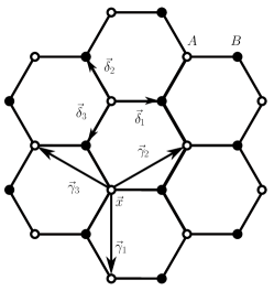
Figure 3: The honeycomb lattice of the Haldane-Hubbard model.

Correlations, current and conductivity. It is convenient to define

$$\Psi^{+}_{\vec{x},\sigma}=\big{(}a^{+}_{\vec{x},\sigma},\,b^{+}_{\vec{x}+\vec{\delta}_{1},\sigma}\big{)}\;,\qquad\Psi^{-}_{\vec{x},\sigma}=\big{(}\Psi^{+}_{\vec{x},\sigma}\big{)}^{\dagger}\;;$$ (13)

also, for any inverse temperature $\beta$, we let $\Psi^{\pm}_{\vec{x},\sigma}(x_{0})=e^{Hx_{0}}\Psi^{\pm}_{\vec{x},\sigma}e^{-Hx_{0}}$ be their evolution at ‘imaginary time’ $x_{0}\in[0,\beta)$. For general $x_{0}\in\mathbb{R}$, we extend $\Psi^{\pm}_{\vec{x},\sigma}(x_{0})$ anti-periodically (of anti-period $\beta$) beyond the basic interval $[0,\beta)$. The Fourier transform of the fields is defined as $\Psi^{\pm}_{\vec{x},\sigma}=\int_{\cal B}\frac{d\vec{k}}{|{\cal B}|}e^{\pm i\vec{k}\cdot\vec{x}}\hat{\Psi}^{\pm}_{\vec{k},\sigma}$, where ${\cal B}$ is the Brillouin zone brillouin . The 2-point function is

$$S_{2}({\bf x},{\bf y}) = {\langle{\bf T}\,\Psi^{-}_{\vec{x},\sigma}(x_{0})\Psi^{+}_{\vec{y},\sigma}(y_{0})\rangle}$$

$$= \int_{\mathbb{R}\times{\cal B}}\frac{d{\bf k}}{2\pi|{\cal B}|}e^{-i{\bf k}({\bf x}-{\bf y})}\hat{S}_{2}({\bf k}),$$

where ${\bf x}=(x_{0},\vec{x})$, ${\bf y}=(y_{0},\vec{y})$, ${\bf T}$ is the fermionic time-ordering operator (which orders imaginary times in decreasing order order ), and ${\bf k}=(k_{0},\vec{k})$, where $k_{0}$ is the Matsubara frequency. Note that $S_{2}$ is a $2\times 2$ matrix (with indices in the ‘sublattice’ space) and its definition is independent of the choice of $\sigma=\uparrow,\downarrow$.

The current is defined via the Peierls’ substitution (see App.A), and is equal to

$$\vec{J}_{\vec{p}}(x_{0})=\sum_{\sigma=\uparrow\downarrow}\int_{{\cal B}}\frac{d\vec{k}}{|{\cal B}|}\hat{\Psi}^{+}_{\vec{k}+\vec{p},\sigma}(x_{0})\vec{M}(\vec{k},\vec{p})\hat{\Psi}^{-}_{\vec{k},\sigma}(x_{0})\;.$$ (14)

The two components $M_{i}(\vec{k},\vec{p})$, $i=1,2$, of $\vec{M}(\vec{k},\vec{p})$ are the bare vertex functions, which are $2\times 2$ matrices, with elements labelled by the spinor indices. For the explicit expression of the bare vertex functions, see App.A.

The current-current and the vertex correlations are defined, respectively, as

$$\hat{K}_{\mu\nu}({\bf p})=\int_{\mathbb{R}}dx_{0}e^{-ip_{0}x_{0}}{\langle\!\!\langle{\bf T}\,J_{\vec{p},\mu}(x_{0});J_{-\vec{p},\nu}(0)\rangle\!\!\rangle}_{\!\infty},$$

$$\hat{G}_{\mu}({\bf k},{\bf p})=\int_{\mathbb{R}}dx_{0}\int_{\mathbb{R}}dy_{0}\,e^{-ip_{0}x_{0}+i(k_{0}+p_{0})y_{0}}\times$$

$$\hskip 34.14322pt\times{\langle\!\!\langle{\bf T}\,J_{\vec{p},\mu}(x_{0});\hat{\Psi}^{-}_{\vec{k}+\vec{p},\sigma}(y_{0})\hat{\Psi}^{+}_{\vec{k},\sigma}\rangle\!\!\rangle}_{\!\infty},$$ (15)

where $\mu,\nu\in\{0,1,2\}$,

$$J_{\vec{p},0}(x_{0})=\sum_{\vec{x}\in\Lambda_{A}}\sum_{\sigma=\uparrow\downarrow}e^{-i\vec{p}\cdot\vec{x}}\Psi^{+}_{\vec{x},\sigma}(x_{0})M_{0}(\vec{p})\Psi^{-}_{\vec{x},\sigma}(x_{0}),$$

with

$$M_{0}(\vec{p})=\begin{pmatrix}1&0\\ 0&e^{-i\vec{p}_{1}}\end{pmatrix}\;;$$ (16)

the labels $\mu=1,2$ refer to the components of the current defined in Eq. (14). Moreover, ${\langle\!\!\langle\cdot\rangle\!\!\rangle}_{\!\infty}=\lim_{\beta\to\infty}\lim_{L\to\infty}L^{-2}{\langle\cdot\rangle}_{\beta,L}$ is the trace per unit volume, and the semi-colon indicates that the expectation is truncated.

For later reference, we also introduce the vertex function:

$$\hat{\Gamma}_{\mu}({\bf k},{\bf p})=\hat{S}_{2}^{-1}({\bf k}+{\bf p})\hat{G}_{\mu}({\bf k},{\bf p})\hat{S}_{2}^{-1}({\bf k}),$$ (17)

where $\hat{S}_{2}^{-1}({\bf k})$ is the inverse of the 2-point function, thought of as a $2\times 2$ matrix.

Finally, the d.c. Kubo conductivity is defined in terms of the current-current correlation, in units such that $e^{2}=\hbar=1$, as:

$$\sigma_{ij}=-\lim_{p_{0}\rightarrow 0^{+}}\frac{1}{Ap_{0}}\big{[}\hat{K}_{ij}(p_{0},0)-\hat{K}_{ij}({\bf 0})\big{]},$$ (18)

where $i,j=1,2$ and $A=|\vec{\ell}_{1}\times\vec{\ell}_{2}|=3\sqrt{3}/2$ is the area of the fundamental cell.

Ward Identities. The continuity equation for the lattice current Eq. (14), when averaged against an arbitrary number of field operators, implies exact identities among correlation functions (Ward Identities), valid for any value of the interaction $U$. In particular, the one relating the 2-point and the vertex functions, which will play an important role in the following, reads as follows:

$$\sum_{\mu=0}^{2}(i)^{\delta_{\mu,0}}p_{\mu}\hat{G}_{\mu}({\bf k},{\bf p})=\hat{S}_{2}({\bf k}+{\bf p})M_{0}(\vec{p})-M_{0}(\vec{p})\hat{S}_{2}({\bf k}).$$ (19)

If we derive this equation with respect to ${\bf p}$, compute the result at ${\bf p}={\bf 0}$ and recall the definition (17) of the vertex function, we find:

$$\hat{\Gamma}_{\mu}({\bf k},{\bf 0})=(-i)^{\delta_{\mu,0}}\partial_{\mu}\hat{S}_{2}^{-1}({\bf k})+\big{[}\partial_{\mu}M_{0}(\vec{0}),\hat{S}_{2}^{-1}({\bf k})\big{]}.$$ (20)

In the following, $\hat{\Gamma}_{\mu}({\bf k},{\bf 0})$ will be denoted simply by $\hat{\Gamma}_{\mu}({\bf k})$.

The non-interacting case. If $U=0$, the band structure and the phase diagram can be computed explicitly: the Bloch Hamiltonian is H

$$\hat{H}_{0}(\vec{k})=$$ (21)

$$\quad=\begin{pmatrix}-2t_{2}\cos\phi\,\alpha_{1}(\vec{k})+m(\vec{k})&-t_{1}\Omega^{*}(\vec{k})\\ -t_{1}\Omega(\vec{k})&\hskip-8.5359pt-2t_{2}\cos\phi\,\alpha_{1}(\vec{k})-m(\vec{k})\end{pmatrix}$$

where $\Omega(\vec{k})=1+e^{-i\vec{k}\cdot\vec{\ell}_{1}}+e^{-i\vec{k}\cdot\vec{\ell}_{2}}$ and

$$\alpha_{1}(\vec{k})=\sum_{i=1}^{3}\cos(\vec{k}\cdot\vec{\gamma}_{i})\;,\quad\alpha_{2}(\vec{k})=\sum_{i=1}^{3}\sin(\vec{k}\cdot\vec{\gamma}_{i})$$

$$m(\vec{k})=W-2t_{2}\sin\phi\,\alpha_{2}(\vec{k})\;.$$ (22)

The corresponding energy bands are

$$\varepsilon_{\pm}(\vec{k})=-2t_{2}\cos\phi\,\alpha_{1}(\vec{k})\pm\sqrt{m(\vec{k})^{2}+t_{1}^{2}|\Omega(\vec{k})|^{2}}\;.$$

To make sure that the energy bands do not overlap, we assume that $t_{2}/t_{1}<1/3$. The two bands can only touch at the Fermi points $\vec{p}_{F}^{\pm}=\big{(}\frac{2\pi}{3},\pm\frac{2\pi}{3\sqrt{3}}\big{)}$, which are the two zeros of $\Omega(\vec{k})$, around which $\Omega(\vec{p}_{F}^{\pm}+\vec{k}^{\prime})\simeq\frac{3}{2}(ik_{1}^{\prime}\pm k_{2}^{\prime})$. The condition that the two bands touch at $\vec{p}_{F}^{\omega}$, with $\omega=+,-$, is that $m_{\omega}=0$, with

$$m_{\omega}\equiv m(\vec{p}_{F}^{\omega})=W+\omega 3\sqrt{3}\,t_{2}\sin\phi\;.$$

Therefore, the unperturbed critical curves are given by the values of $(\phi,W)$ such that:

$$W=\pm 3\sqrt{3}\,t_{2}\sin\phi\,,$$ (23)

which correspond to the dotted curves in Fig.1. Fixing the chemical potential in such a way that the Fermi energy lies in between the two bands,

$$\mu=-2t_{2}\cos\phi\,\alpha_{1}(\vec{p}_{F}^{\pm})=-3t_{2}\cos\phi\;,$$ (24)

the system passes from a semi-metallic behavior, when $(\phi,W)$ is on the critical line, to an insulating behavior, characterized by the exponential decay of correlations, when $W\not=\pm 3\sqrt{3}t_{2}\,\sin\phi$.

The insulating phase consists of four disconnected regions in the $(\phi,W)$ plane, two of which are ‘topologically trivial’, while the other two have non-zero Hall conductivity, see Fig.1: more precisely, if $W\not=\pm 3\sqrt{3}t_{2}\,\sin\phi$,

$$\sigma_{12}=\frac{\nu}{2\pi}\;,\quad\nu=\text{sign}(m_{-})-\text{sign}(m_{+})\;.$$

III Renormalization Group analysis

We now construct the interacting correlations and phase diagram, by using a convergent renormalized expansion, in the spirit of Ref.GM ; GMP ; GMPhall . In this section, we introduce the functional integral formulation of the model, discuss the exact lattice symmetries of the fermionic action, and describe the infrared integration, including the study of the flow of the running coupling constants. One of the main results of this section is the equation for the interacting critical line.

III.1 Functional integral formulation

We are interested in the semi-metallic and insulating regimes of the interacting system. We, therefore, set the chemical potential accordingly (its value will be different, in general, from the unperturbed one):

$$\mu=-2t_{2}\cos\phi\,\alpha_{1}(\vec{p}_{F}^{\pm})-\xi,$$

where $\xi$ (the shift of the chemical potential) must be chosen as a function of $U,W,\phi,$ so that the renormalized propagator either has a linear, ‘conical’, infrared singularity (along the interacting critical line), or is gapped (in the insulating phase).

The generating function ${\cal W}(f,A)$ for correlations, in which $f$ is the external field conjugated to the fermionic fields, and $A$ is the external field conjugated to the current, can be written as the following Grassmann integral:

$$e^{{\cal W}(f,A)}=\frac{\int P(d\psi)e^{-V(\psi)+(\psi,f)+(j,A)}}{\int P(d\psi)e^{-V(\psi)}},$$ (25)

where: $\psi^{\pm}_{{\bf x},\sigma}$, with ${\bf x}=(x_{0},\vec{x})\in\mathbb{R}\times\Lambda_{A}$ and $\sigma\in\{\uparrow,\downarrow\}$, is a two-component Grassmann spinor (it is the Grassmann counterpart of $\Psi^{\pm}_{\vec{x},\sigma}(x_{0})$), whose components will be denoted by $\psi^{\pm}_{{\bf x},\sigma,\rho}$, with $\rho=1,2$; $P(d\psi)$ is the fermionic Gaussian integration with propagator

$$g({\bf x},{\bf y})=\int_{\mathbb{R}\times{\cal B}}\frac{d{\bf k}}{2\pi|{\cal B}|}e^{-i{\bf k}({\bf x}-{\bf y})}\hat{g}({\bf k}),$$ (26)

where, letting $R(\vec{k})=-2t_{2}\cos\phi\big{(}\alpha_{1}(\vec{k})-\alpha_{1}(\vec{p}_{F}^{\pm})\big{)}$,

$$\hat{g}({\bf k})=\begin{pmatrix}&-ik_{0}+R(\vec{k})+m(\vec{k})&-t_{1}\Omega^{*}(\vec{k})\\ &-t_{1}\Omega(\vec{k})&-ik_{0}+R(\vec{k})-m(\vec{k})\end{pmatrix}^{\!\!\!-1}$$

and, at contact, $g({\bf x},{\bf x})$ should be interpreted as $\lim_{\varepsilon\to 0^{+}}[g({\bf x}+(\varepsilon,\vec{0}),{\bf x})+g({\bf x}-(\varepsilon,\vec{0}),{\bf x})]$;

$$V(\psi)=\int_{\mathbb{R}}dx_{0}\sum_{\vec{x}\in\Lambda_{A}}\sum_{\rho=1,2}\big{(}Un^{\rho}_{{\bf x},\uparrow}n^{\rho}_{{\bf x},\downarrow}+\xi\sum_{\sigma=\uparrow,\downarrow}n^{\rho}_{{\bf x},\sigma}\big{)},$$

where $n^{\rho}_{{\bf x},\sigma}=\psi^{+}_{{\bf x},\sigma,\rho}\psi^{-}_{{\bf x},\sigma,\rho}$; and, finally,

$$(\psi,f)=\int_{\mathbb{R}}dx_{0}\sum_{\vec{x}\in\Lambda_{A}}\sum_{\sigma=\uparrow\downarrow}(\psi^{+}_{{\bf x},\sigma}f^{-}_{{\bf x},\sigma}+f^{+}_{{\bf x},\sigma}\psi^{-}_{{\bf x},\sigma}),$$

$$(j,A)=\int_{\mathbb{R}^{3}}\frac{d{\bf p}}{(2\pi)^{3}}\hat{A}_{{\bf p},\mu}\hat{\jmath}_{{\bf p},\mu},$$

where $\hat{\jmath}_{{\bf p},\mu}=\sum_{\sigma=\uparrow\downarrow}\int_{\mathbb{R}\times{\cal B}}\frac{d{\bf k}}{2\pi|{\cal B}|}\hat{\psi}^{+}_{{\bf k}+{\bf p},\sigma}\Gamma_{\mu}(\vec{k},\vec{p})\hat{\psi}^{-}_{{\bf k},\sigma}$, in which $\Gamma_{\mu}(\vec{k},\vec{p})$ are the bare vertex functions, namely: $\Gamma_{0}(\vec{k},\vec{p})=M(\vec{p})$, and, if $i=1,2$, $\Gamma_{i}(\vec{k},\vec{p})$ are the two components of the (matrix-valued) vector $\vec{M}(\vec{k},\vec{p})$ defined in (14) and following lines. In terms of these definitions, the correlations can be re-expressed as

$$S_{2}({\bf x},{\bf y}) = \frac{\partial^{2}\mathcal{W}}{\partial f^{+}_{{\bf x},\sigma}\partial f^{-}_{{\bf y},\sigma}}(0,0)\;,$$

$$K_{\mu\nu}({\bf x},{\bf y}) = \frac{\partial^{2}\mathcal{W}}{\partial j_{{\bf x},\mu}\partial j_{{\bf y},\nu}}(0,0)\;,$$ (27)

and of suitable linear combinations of

$$G_{2,1;\mu}({\bf x},{\bf y},{\bf z})=\frac{\partial^{3}\mathcal{W}}{\partial A_{{\bf x},\mu}\partial f^{+}_{{\bf y},\sigma}\partial f^{-}_{{\bf z},\sigma}}(0,0)\;.$$ (28)

We now compute the generating function Eq. (25) via a renormalized expansion, which is convergent uniformly close to (and even on) the critical line. Note that, on this line, the Grassmann integral has an infrared problem. In order to resolve and re-sum the corresponding singularities, we proceed in a multi-scale fashion. First of all, we distinguish the ultraviolet modes, corresponding to large values of the Matsubara frequency, from the infrared ones, by introducing two compactly supported cut-off functions, $\chi_{\pm}({\bf k})$, supported in the vicinity of the Fermi points (more precisely, we let $\chi_{\pm}({\bf k})=\chi_{0}({\bf k}-{\bf p}_{F}^{\pm})$, where $\chi_{0}$ is a smoothed out characteristic function of the ball of radius $a_{0}$, with $a_{0}$ equal to, say, $1/3$, and ${\bf p}_{F}^{\pm}=(0,\vec{p}_{F}^{\pm})$) and by letting $\chi_{uv}({\bf k})=1-\sum_{\omega=\pm}\chi_{\omega}({\bf k})$. We correspondingly split the propagator in its ultraviolet and infrared components:

$$g({\bf x},{\bf y})=g^{(1)}({\bf x},{\bf y})+\sum_{\omega=\pm}e^{-i\vec{p}_{F}^{\omega}(\vec{x}-\vec{y})}g_{\omega}^{(\leq 0)}({\bf x},{\bf y})$$ (29)

where $g^{(1)}({\bf x},{\bf y})$ and $g_{\omega}^{(\leq 0)}({\bf x},{\bf y})$ are defined in a similar way as Eq. (26), with $\hat{g}({\bf k})$ replaced by $\chi_{uv}({\bf k})\hat{g}({\bf k})$ and by $\chi_{0}({\bf k})\hat{g}({\bf k}+{\bf p}_{F}^{\omega})$, respectively. We then split the Grassmann field as a sum of two independent fields, with propagators $g^{(1)}$ and $g^{(\leq 0)}$:

$$\psi_{{\bf x},\sigma}^{\pm}=\psi^{\pm(1)}_{{\bf x},\sigma}+\sum_{\omega=\pm}e^{\pm i\vec{p}_{F}^{\omega}\vec{x}}\psi_{{\bf x},\sigma,\omega}^{\pm(\leq 0)}$$

and we rewrite the Grassmann Gaussian integration as the product of two independent Gaussians: $P(d\psi)=P(d\psi^{(\leq 0)})P(\psi^{(1)})$. By construction, the integration of the ‘ultraviolet’ field $\psi^{(1)}$ does not have any infrared singularity and, therefore, can be performed in a straightforward manner, thus allowing us to rewrite the generating function $\mathcal{W}(f,A)$ as the logarithm of

$$\frac{e^{{\cal W}^{(0)}(f,A)}}{\mathcal{N}_{0}}\int P(d\psi^{(\leq 0)})e^{-V^{(0)}(\psi^{(\leq 0)})+B^{(0)}(\psi^{(\leq 0)},f,A)},$$ (30)

where $V^{(0)}$ and $B^{(0)}$ are, respectively, the effective potential and the effective source (which depend explicitly on, respectively, $\psi^{(\leq 0)}$ and $\psi^{(\leq 0)},f,A$), ${\cal W}^{(0)}$ is independent of $\psi^{(\leq 0)}$ (and depends explicitly on $f,A$), and $\mathcal{N}_{0}=\int P(d\psi^{(\leq 0)})e^{-V^{(0)}(\psi^{(\leq 0)})}$. Both $V^{(0)}$ and $B^{(0)}$ are expressed as series of monomials in the $\psi,f,A$ fields, whose kernels (given by the sum of all possible Feynman diagrams with fixed number and fixed location of the external legs) are analytic functions of the interaction strength, for $U$ sufficiently small. The proof of their analyticity is based on a determinant expansion and on a systematic use of the Gram-Hadamard bounds, see Ref.GM ; GMPhall .

III.2 Symmetries

Before tackling the multi-scale integration of the infrared modes, we make a digression about the symmetry structure of the effective potential, and in particular of its local parts: the purpose is to classify the possible relevant and marginal coupling constants. In the case $t_{2}=W=\mu=0$ (standard graphene model) the lattice symmetries severely constrain the form of the quadratic terms in the effective potential: in particular, the interaction does not shift the chemical potential, nor does it generate a massGM ; GMP ; FA ; HJR . In the general case ($W,t_{2},\phi\neq 0$) the model is invariant under the following symmetry transformations (since they do not mix the spin indices, for notational convenience we temporarily drop the spin labels from the formulas).

We discuss the symmetries in the absence of external fields, since we will use them only to infer the structure of the relevant and marginal contributions to the effective potential $V^{(0)}$. Once the structure of these terms is known, the structure of the marginal contributions to the effective source $B^{(0)}$ can be computed by using the Ward Identity (20).

(1) Discrete rotations:

$$\hat{\psi}_{{\bf k}}^{-}\to e^{i\vec{k}(\vec{\delta}_{3}-\vec{\delta}_{1})n_{-}}\hat{\psi}_{T{\bf k}}^{-}\;,\quad\hat{\psi}_{{\bf k}}^{+}\to\hat{\psi}_{T{\bf k}}^{+}e^{-i\vec{k}(\vec{\delta}_{3}-\vec{\delta}_{1})n_{-}}$$ (31)

where, denoting the Pauli matrices by $\sigma_{1},\sigma_{2},\sigma_{3}$, we defined

$$n_{-}=(1-\sigma_{3})/2\;,\qquad T{\bf k}=(k_{0},e^{-i\frac{2\pi}{3}\sigma_{2}}\vec{k})\;;$$ (32)

that is, $T$ is the spatial rotation by $2\pi/3$ in the counter-clockwise direction.

(2) Complex conjugation:

$$\hat{\psi}^{\pm}_{{\bf k}}\rightarrow\hat{\psi}^{\pm}_{-{\bf k}}\;,$$ (33)

combined with

$$c\rightarrow c^{*}\;,\quad\phi\to-\phi\;,$$ (34)

where $c$ is a generic constant appearing in $P(d\psi)$ or in $V(\psi)$.

(3) Horizontal reflections:

$$\hat{\psi}^{-}_{{\bf k}}\to\sigma_{1}\hat{\psi}^{-}_{R_{h}{\bf k}}\;,\quad\hat{\psi}^{+}_{{\bf k}}\to\hat{\psi}^{+}_{R_{h}{\bf k}}\sigma_{1}\;,$$ (35)

with

$$R_{h}{\bf k}=(k_{0},-k_{1},k_{2})\,,\quad(W,\phi)\to(-W,-\phi)$$ (36)

(4) Vertical reflections:

$$\hat{\psi}^{\pm}_{{\bf k}}\rightarrow\hat{\psi}^{\pm}_{R_{v}{\bf k}}\,,$$ (37)

with

$$R_{v}{\bf k}=(k_{0},k_{1},-k_{2})\;,\quad\phi\to-\phi.$$ (38)

(5) Particle-hole:

$$\hat{\psi}^{-}_{{\bf k}}\to i\hat{\psi}^{+,T}_{P{\bf k}}\;,\quad\hat{\psi}^{+}_{{\bf k}}\to i\hat{\psi}^{-,T}_{P{\bf k}}\;,$$ (39)

with

$$P{\bf k}=(k_{0},-k_{1},-k_{2})\;,\quad\phi\to-\phi\;.$$ (40)

Note that, at fixed $W,\phi$, the theory is invariant under the transformations (1), (2)+(4), and (2)+(5). In particular, these transformations leave the quadratic part $Q^{(0)}(\psi)=\sum_{\sigma}\int\frac{d{\bf k}}{(2\pi|{\cal B}|)}\hat{\psi}^{+}_{{\bf k},\sigma}\hat{W}_{2}({\bf k})\hat{\psi}^{-}_{{\bf k},\sigma}$ of the effective potential $V^{(0)}(\psi)$ invariant. This means that:

$$\hat{W}_{2}({\bf k}) = e^{-i\vec{k}(\vec{\delta}_{1}-\vec{\delta}_{2})n_{-}}\hat{W}_{2}(T^{-1}{\bf k})e^{i\vec{k}(\vec{\delta}_{1}-\vec{\delta}_{2})n_{-}}$$

$$= \hat{W}_{2}^{*}(-k_{0},-k_{1},k_{2})$$

$$= \hat{W}_{2}^{\dagger}(-k_{0},k_{1},k_{2}).$$

As we will see in the next section, the values of $\hat{W}_{2}({\bf k})$ and of its derivatives at the Fermi points define the effective coupling constants. By (III.2), we find, for $\omega=\pm$,

$$\hskip-5.69046pt\hat{W}_{2}({\bf p}_{F}^{\omega}) = e^{-i\frac{2\pi}{3}\omega n_{-}}\hat{W}_{2}({\bf p}_{F}^{\omega})e^{i\frac{2\pi}{3}\omega n_{-}}$$

$$= \hat{W}_{2}^{*}({\bf p}_{F}^{\omega})=\hat{W}_{2}^{\dagger}({\bf p}_{F}^{\omega}),$$

which implies that

$$\hat{W}_{2}({\bf p}_{F}^{\omega})=\xi_{\omega}+\delta_{\omega}\sigma_{3},$$ (42)

for two real constants $\xi_{\omega}$ and $\delta_{\omega}$.

If we derive (III.2) with respect to ${\bf k}$ and compute the result at ${\bf p}_{F}^{\omega}$, we find:

$$\partial_{\bf k}\hat{W}_{2}({\bf p}_{F}^{\omega}) = e^{-i\frac{2\pi}{3}\omega n_{-}}T\partial_{\bf k}\hat{W}_{2}({\bf p}_{F}^{\omega})e^{i\frac{2\pi}{3}\omega n_{-}}$$

$$= (-R_{v})\partial_{\bf k}\hat{W}_{2}^{*}({\bf p}_{F}^{\omega})$$

$$= (-P)\partial_{\bf k}\hat{W}_{2}^{\dagger}({\bf p}_{F}^{\omega}),$$

where $R_{v}$ (resp. $P$) is the diagonal matrix with diagonal elements $(1,1,-1)$ (resp. $(1,-1,-1)$). By using (III.2), it is straightforward to check that

$${\bf k}^{\prime}\partial_{{\bf k}}\hat{W}({\bf p}_{F}^{\omega})=\begin{pmatrix}-iz_{1,\omega}k_{0}&-u_{\omega}(-ik_{1}^{\prime}+\omega k_{2}^{\prime})\\ -u_{\omega}(ik_{1}^{\prime}+\omega k_{2}^{\prime})&-iz_{2,\omega}k_{0}\end{pmatrix},$$ (44)

where ${\bf k}^{\prime}={\bf k}-{\bf p}_{F}^{\omega}=(k_{0},\vec{k^{\prime}})$, and $u_{\omega},z_{1,\omega},z_{2,\omega}$ are real constants. In conclusion, for general values of $W,\phi$, the linearization of $\hat{W}_{2}({\bf k})$ at ${\bf p}_{F}^{\omega}$ is parametrized by 5 real constants, namely $\xi_{\omega},\delta_{\omega},u_{\omega},z_{1,\omega}$ and $z_{2,\omega}$, the first two are relevant coupling constants, and the other three are marginal. Note that, in general, the values of these constants depend on $\omega$ (therefore, there are 5 of them at ${\bf p}_{F}^{+}$ and 5 more at ${\bf p}_{F}^{-}$). Note also that, in general, $z_{1,\omega}\neq z_{2,\omega}$, i.e., the wave function renormalization depends explicitly on the spinor index, an effect that can be checked explicitly at second order in perturbation theory (see below), and cannot be explained purely in terms of the relativistic approximation of the model around the Fermi points.

Note that there are special points in the $(W,\phi)$ plane, for which the model has more symmetries, and where the number of independent couplings is smaller than in the general case. For instance, if $W=\phi=0$, the model is invariant under all the 5 symmetry transformations listed above, in which case it is straightforward to see that

$$\xi_{\omega}=\xi_{-\omega}\;,\quad\delta_{\omega}=0\;,\quad u_{\omega}=u_{-\omega}\;,$$

$$z_{1,\omega}=z_{2,\omega}=z_{1,-\omega}=z_{2,-\omega}\;.$$ (45)

A similar discussion applies to the case $W=0$, $\phi=\pi$.

Finally, if $\phi=\pi/2$, the model is invariant under the following additional symmetry transformation (see also Ref.Z ):

$$\hat{\psi}^{-}_{{\bf k},\sigma}\to-i\sigma_{1}\sigma_{3}\hat{\psi}^{-}_{-R_{v}{\bf k},\sigma}\;,\quad\hat{\psi}^{+}_{{\bf k},\sigma}\to-i\hat{\psi}^{+}_{-R_{v}{\bf k},\sigma}\sigma_{3}\sigma_{1}\;,$$ (46)

which implies that

$$\hat{W}_{2}({\bf k})=-\sigma_{3}\sigma_{1}\hat{W}_{2}(-k_{0},-k_{1},k_{2})\sigma_{1}\sigma_{3},$$

so that, in particular,

$$\xi_{\omega}=0\;,\quad z_{1,\omega}=z_{2,\omega}\;.$$ (47)

A similar discussion applies to $\phi=-\pi/2$.

III.3 Infrared integration

Let us now describe the integration of the infrared fields. We shall focus on the semi-metallic behavior of the system at, or very close to, a generic point of the critical line. Moreover, since we are interested in the behavior of the current-current correlations around ${\bf p}={\bf 0}$, we shall assume that the external field $\hat{A}_{{\bf p},\mu}$ is supported in the vicinity of the origin (in particular, we assume that it vanishes in the vicinity of ${\bf p}_{F}^{\omega}-{\bf p}_{F}^{-\omega}$, $\omega=\pm$).

By dimensional considerations, the quadratic terms in the effective action are relevant, and, the ones corresponding to the renormalization of the mass are of particular importance. The flow of the effective mass tends to diverge linearly under the RG iterations, which signals that, in general, the location of the critical lines is changed by the interaction. In order to construct a convergent expansion, we need to dress the mass, after which we determine the location of the renormalized critical lines, which is given by the condition that the dressed mass vanishes.

More in detail, we proceed as follows. We perform the integration of the infrared modes in (30) iteratively, by decomposing the fermionic fields as $\psi_{{\bf x},\sigma,\omega}^{\pm(\leq 0)}$ as $\psi_{{\bf x},\sigma,\omega}^{\pm(\leq 0)}=\sum_{h\leq 0}\psi_{{\bf x},\sigma,\omega}^{\pm(h)}$, where $\psi_{{\bf x},\sigma,\omega}^{\pm(h)}$ is a Grassmann field whose propagator is supported on the momenta ${\bf k}$ such that $|{\bf k}-{\bf p}_{F}^{\omega}|\sim 2^{h}$, and by integrating the fields $\psi^{(0)},\psi^{(-1)},\ldots$ step by step. After the integration of the modes on scales $0,-1,\ldots,h+1$, we rewrite the generating function ${\cal W}(f,A)$ as the logarithm of

$$\frac{e^{{\cal W}^{(h)}(f,A)}}{\mathcal{N}_{h}}\int P(d\psi^{(\leq h)})e^{-V^{(h)}(\psi^{(\leq h)})+B^{(h)}(\psi^{(\leq h)},f,A)},$$ (48)

where $V^{(h)}$ and $B^{(h)}$ are, respectively, the effective potential and source terms, to be defined inductively in the following. Moreover, $P(d\psi^{(\leq h)})$ is the Grassmann Gaussian integration with propagator (diagonal with respect to the $\sigma$ and $\omega$ indices)

$$g^{(\leq h)}_{\omega}({\bf x},{\bf y}) = \int P(d\psi^{(\leq h)})\psi^{-(\leq h)}_{{\bf x},\sigma,\omega}\psi^{+(\leq h)}_{{\bf y},\sigma,\omega}$$

$$= \int\frac{d{\bf k}^{\prime}}{2\pi|{\cal B}|}e^{-i{\bf k}^{\prime}({\bf x}-{\bf y})}\hat{g}_{\omega}^{(\leq h)}({\bf k}^{\prime}),$$

where ${\bf k}^{\prime}=(k_{0},\vec{k}^{\prime})$ and, letting $r_{\omega}(\vec{k}^{\prime})=R(\vec{k}^{\prime}+\vec{p}_{F}^{\omega})$, $s_{\omega}(\vec{k}^{\prime})=-t_{1}[\Omega(\vec{k}^{\prime}+\vec{p}_{F}^{\,\omega})-\frac{3}{2}(ik_{1}^{\prime}+\omega k_{2}^{\prime})]$ and $\chi_{h}({\bf k}^{\prime})=\chi_{0}(2^{-h}{\bf k}^{\prime})$ (here $\chi_{0}$ is the cutoff function defined a few lines before (29)),

$$\hat{g}_{\omega}^{(\leq h)}({\bf k})=\chi_{h}({\bf k}^{\prime})\begin{pmatrix}a_{1,\omega,h}({\bf k}^{\prime})&b^{*}_{\omega,h}({\bf k}^{\prime})\\ b_{\omega,h}({\bf k}^{\prime})&a_{2,\omega,h}({\bf k}^{\prime})\end{pmatrix}^{\!\!\!-1},$$ (49)

with

$$a_{\rho,\omega,h}({\bf k})=-ik_{0}Z_{\rho,\omega,h}+r_{\omega}(\vec{k}^{\prime})+(-1)^{\rho-1}m_{\omega,h}(\vec{k}^{\prime}),$$

$$b_{\omega,h}({\bf k}^{\prime})=-v_{\omega,h}(ik_{1}^{\prime}+\omega k_{2}^{\prime})+s_{\omega}(\vec{k}^{\prime})\;.$$ (50)

in which $Z_{j,\omega,h}$, $m_{\omega,h}(\vec{k}^{\prime})$ and $v_{\omega,h}$ are, respectively, the wave function renormalizations, the effective mass and effective velocities, to be defined inductively in the following. Their initial values are:

$$Z_{j,\omega,0}=1\;,\quad m_{\omega,0}(\vec{k}^{\prime})=m(\vec{k}^{\prime}+\vec{p}_{F}^{\,\omega})\;,\quad v_{\omega,0}=\frac{3}{2}t_{1}.$$ (51)

In order to clarify the inductive definition of the effective potential, source, etc, we now describe the integration step at scale $h$. We start from (48), where $V^{(h)}(\psi)$ is a sum of even monomials in the $\psi$ fields, whose kernels of order $n$ are denoted by $W^{(h)}_{n}$ (for notational simplicity, we temporarily drop the space-time, spin, spinor and valley indices of the fermionic fields). Similarly, we denote the kernels of $B^{(h)}$ of order $n$ in $\psi$, $m$ in $f$ and $q$ in $A$, by $W_{n,m,q}$. The scaling dimension of the kernels $W_{n}$ and $W_{n,m,q}$ is (see Ref.GM ; GMP ; GMPhall )

$$D=3-n-m-q,$$ (52)

with the convention that $D>0$ corresponds to relevant, $D=0$ to marginal, and $D<0$ to irrelevant operators. Note that the only relevant terms are those with $n+m=2$, and the only marginal terms are those with $n+m=2$ and $q=1$ (note that, by construction, $n+m$ is positive and even). In particular, the effective electron-electron interaction, corresponding to the case $n=4$ and $m=q=0$, is irrelevant.

In order to define a convergent renormalized expansion, we need to re-sum the relevant and marginal terms. For this purpose, we split $V^{(h)}$ and $B^{(h)}$ into their local and irrelevant parts (here, for simplicity, we spell out the definitions only in the $f=0$ case, the general case is treatable analogously, along the lines of, e.g., Sect. 12 of Ref.GeM , or Ref.GMP ): $V^{(h)}={\cal L}V^{(h)}+{\cal R}V^{(h)}$ and $B^{(h)}={\cal L}B^{(h)}+{\cal R}B^{(h)}$, where, denoting the quadratic part of $V^{(h)}$ by

$$\sum_{\omega,\sigma}\int\frac{d{\bf k}^{\prime}}{2\pi|{\cal B}|}\hat{\psi}^{+}_{{\bf k}^{\prime},\sigma,\omega}\hat{W}^{(h)}_{2;\omega}({\bf k}^{\prime})\hat{\psi}^{-}_{{\bf k}^{\prime},\sigma,\omega},$$

and the part of $B^{(h)}$ of order $(2,0,1)$ in $(\psi,f,A)$ by

$$\sum_{\omega,\sigma}\int\frac{d{\bf p}}{(2\pi)^{3}}\int\frac{d{\bf k}^{\prime}}{2\pi|{\cal B}|}\hat{A}_{-{\bf p},\mu}\hat{\psi}^{+}_{{\bf k}^{\prime}+{\bf p},\sigma,\omega}\hat{W}^{(h)}_{2,1;\mu,\omega}({\bf k}^{\prime},{\bf p})\hat{\psi}^{-}_{{\bf k}^{\prime},\sigma,\omega}$$

we let:

$${\cal L}V^{(h)}(\psi)=\sum_{\omega=\pm}\sum_{\sigma=\uparrow\downarrow}\int\frac{d{\bf k}^{\prime}}{2\pi|{\cal B}|}\times$$

$$\quad\times\hat{\psi}^{+}_{{\bf k}^{\prime},\sigma,\omega}[\hat{W}^{(h)}_{2;\omega}({\bf 0})+{\bf k}^{\prime}\partial_{{\bf k}^{\prime}}\hat{W}^{(h)}_{2;\omega}({\bf 0})\big{]}\hat{\psi}^{-}_{{\bf k}^{\prime},\sigma,\omega},$$

and

$${\cal L}B^{(h)}(\psi,0,A)=\sum_{\omega=\pm}\sum_{\sigma=\uparrow\downarrow}\sum_{\mu=0}^{2}\int\frac{d{\bf p}}{(2\pi)^{3}}\int\frac{d{\bf k}^{\prime}}{2\pi|{\cal B}|}\times$$

$$\quad\times\hat{A}_{{\bf p},\mu}\hat{\psi}^{+}_{{\bf k}^{\prime}+{\bf p},\sigma,\omega}\hat{W}^{(h)}_{2,1;\mu,\omega}({\bf 0},{\bf 0})\hat{\psi}^{-}_{{\bf k}^{\prime},\sigma,\omega}.$$

By the symmetries discussed in the previous section (see, in particular, (42) and (44))

$${\cal L}V^{(h)}(\psi)=\sum_{\omega=\pm}\int\frac{d{\bf k}^{\prime}}{2\pi|{\cal B}|}\Big{[}2^{h}\xi_{\omega,h}\hat{\psi}^{+}_{{\bf k}^{\prime},\sigma,\omega}\hat{\psi}^{-}_{{\bf k}^{\prime},\sigma,\omega}+$$ (53)

$$+\hat{\psi}^{+}_{{\bf k}^{\prime},\sigma,\omega}\begin{pmatrix}-iz_{1,\omega,h}k_{0}+\delta_{\omega,h}&-u_{\omega,h}(-ik_{1}^{\prime}+\omega k_{2}^{\prime})\\ -u_{\omega,h}(ik_{1}^{\prime}+\omega k_{2}^{\prime})&-iz_{2,\omega,h}k_{0}-\delta_{\omega,h}\end{pmatrix}\hat{\psi}^{-}_{{\bf k}^{\prime},\sigma,\omega}\Big{]},$$

where $\xi_{\omega,h},\delta_{\omega,h},z_{j,\omega,h},u_{\omega,h}$ are real constants. Moreover, by using the Ward Identity (20), we find that

$${\cal L}B^{(h)}(\psi,0,A)=\sum_{\omega=\pm}\sum_{\sigma=\uparrow\downarrow}\sum_{\mu=0}^{2}\int\frac{d{\bf p}}{(2\pi)^{3}}\int\frac{d{\bf k}^{\prime}}{2\pi|{\cal B}|}\times$$

$$\quad\times\hat{A}_{{\bf p},\mu}\hat{\psi}^{+}_{{\bf k}^{\prime}+{\bf p},\sigma,\omega}\gamma_{\mu,\omega,h}\hat{\psi}^{-}_{{\bf k}^{\prime},\sigma,\omega},$$ (54)

where

$$\gamma_{0,\omega,h} = -\sum_{\rho=1}^{2}(Z_{\rho,\omega,h}+z_{\rho,\omega,h})n_{\rho}$$

$$\gamma_{1,\omega,h} = -(v_{\omega,h}+u_{\omega,h})\sigma_{2}$$

$$\gamma_{2,\omega,h} = -\omega(v_{\omega,h}+u_{\omega,h})\sigma_{1}$$ (55)

in which $n_{\rho}=(1+(-1)^{\rho-1}\sigma_{3})/2$ and $\sigma_{i}$ are the standard Pauli matrices.

Once the effective potential and source have been split into local and irrelevant parts, we combine the part of ${\cal L}V^{(h)}$ in the second line of (53) with the Gaussian integration $P(d\psi^{(\leq h)})$, thus defining a dressed measure $\tilde{P}(d\psi^{(\leq h)})$ whose propagator $\tilde{g}^{(\leq h)}_{\omega}({\bf x},{\bf y})$ is analogous to $g^{(\leq h)}_{\omega}({\bf x},{\bf y})$, with the only difference that the functions $a_{\rho,\omega,h}$, $b_{\omega,h}$ in (49)-(50) are replaced by

$$\tilde{a}_{\rho,\omega,h-1}({\bf k}) = -ik_{0}\tilde{Z}_{\rho,\omega,h-1}({\bf k}^{\prime})+r_{\omega}(\vec{k}^{\prime})$$

$$+(-1)^{\rho-1}\tilde{m}_{\omega,h-1}({\bf k}^{\prime}),$$

$$\tilde{b}_{\omega,h-1}({\bf k}^{\prime}) = -\tilde{v}_{\omega,h-1}({\bf k}^{\prime})(ik_{1}^{\prime}+\omega k_{2}^{\prime})+s_{\omega}(\vec{k}^{\prime}),$$

with

$$\tilde{Z}_{\rho,\omega,h-1}({\bf k}^{\prime})=Z_{\rho,\omega,h}+z_{\rho,\omega,h}\,\chi_{h}({\bf k}^{\prime}),$$

$$\tilde{m}_{\omega,h-1}({\bf k}^{\prime})=m_{\omega,h}(\vec{k}^{\prime})+\delta_{\omega,h}\,\chi_{h}({\bf k}^{\prime}),$$

$$\tilde{v}_{\omega,h-1}({\bf k}^{\prime})=v_{\omega,h}+u_{\omega,h}\,\chi_{h}({\bf k}^{\prime}).$$

Now, by rewriting the support function $\chi_{h}({\bf k}^{\prime})$ in the definition of $\tilde{g}^{(\leq h)}_{\omega}({\bf x},{\bf y})$ as $\chi_{h}({\bf k}^{\prime})=f_{h}({\bf k}^{\prime})+\chi_{h-1}({\bf k}^{\prime})$, we correspondingly rewrite: $\tilde{g}^{(\leq h)}_{\omega}({\bf x},{\bf y})=\tilde{g}^{(h)}_{\omega}({\bf x},{\bf y})+g^{(\leq h-1)}_{\omega}({\bf x},{\bf y})$, where $g^{(\leq h-1)}_{\omega}({\bf x},{\bf y})$ is defined exactly as in (49)-(50), with $h$ replaced by $h-1$, and $Z_{\rho,\omega,h-1},m_{\omega,h-1},v_{\omega,h-1}$ defined by the flow equations:

$$Z_{\rho,\omega,h-1}=Z_{\rho,\omega,h}+z_{\rho,\omega,h},$$

$$m_{\omega,h-1}(\vec{k}^{\prime})=m_{\omega,h}(\vec{k}^{\prime})+\delta_{\omega,h},$$ (56)

$$v_{\omega,h-1}=v_{\omega,h}+u_{\omega,h}.$$

At this point, we integrate the fields on scale $h$, and define:

$$e^{-V^{(h-1)}(\psi)+B^{(h-1)}(\psi,f,A)+w^{(h)}(f,A)}=C_{h}\int\tilde{P}(d\psi^{(h)})\times$$

$$\quad\times e^{-F_{\xi}^{(h)}(\psi^{(h)}+\psi)+{\cal R}V^{(h)}(\psi^{(h)}+\psi)+B^{(h)}(\psi^{(h)}+\psi,f,A)},$$

where $\tilde{P}(d\psi^{(h)})$ is the Gaussian integration with propagator $\tilde{g}^{(h)}_{\omega}$, $F_{\xi}^{(h)}(\psi)=\sum_{\omega}2^{h}\xi_{\omega,h}\int\frac{d{\bf k}^{\prime}}{2\pi|{\cal B}|}\hat{\psi}^{+}_{{\bf k}^{\prime},\sigma,\omega}\hat{\psi}^{-}_{{\bf k}^{\prime},\sigma,\omega}$, and $C_{h}^{-1}=\int\tilde{P}(d\psi^{(h)})e^{-F_{\xi}^{(h)}(\psi^{(h)})+{\cal R}V^{(h)}(\psi^{(h)})}$. Finally, letting $\mathcal{W}^{(h-1)}=\mathcal{W}^{(h)}+w^{(h)}$, we obtain the same expression as (48), with $h$ replaced by $h-1$. This concludes the proof of the inductive step, corresponding to the integration of the fields on scale $h$.

The integration procedure goes on like this, as long as the two effective masses $m_{\pm,h}$ are small, as compared to $2^{h}$. If we are not exactly at the ‘graphene point’ $W=\phi=0$, i.e., if we are close to, or at, any other point on the critical line but the origin, then after a while we reach a scale $h_{1}$ at which $\max_{\omega}|m_{\omega,h_{1}}|\equiv|m_{\omega_{1},h_{1}}|\simeq 2^{h_{1}}$ (possibly, $h_{1}=0$, in the case that $\max_{\omega}|m_{\omega}|$ is of order 1, i.e., if $W,\phi$ are far enough from the graphene point). Note that, once we reach scale $h_{1}$, the field $\psi_{{\bf k}^{\prime},\sigma,\omega_{1}}^{(\leq h_{1})}$ is massive ‘on the right scale’ $2^{h_{1}}$. At that point, we integrate out the field $\psi_{{\bf k}^{\prime},\sigma,\omega_{1}}^{(\leq h_{1})}$ in a single step, and we are left with a (chiral) theory, whose only dynamical degree of freedom is $\psi^{(\leq h_{1})}_{{\bf k}^{\prime},\sigma,\omega_{2}}$, with $\omega_{2}=-\omega_{1}$.

From that scale on, we integrate $\psi^{(\leq h_{1})}_{{\bf k}^{\prime},\sigma,\omega_{2}}=\sum_{h\leq h_{1}}\psi^{(h)}_{{\bf k}^{\prime},\sigma,\omega_{2}}$ in a multi-scale fashion, analogous to the one discussed above, with the important difference that only the running coupling constants corresponding to the valley index $\omega=\omega_{2}$ continue to flow. The multi-scale integration goes on until we reach a scale $h_{2}$ such that $|m_{\omega_{2},h_{2}}|\simeq 2^{h_{2}}$, at which point we can integrate out the remaining degrees of freedom in a single step. The criticality condition, i.e., the condition that the system is on the (renormalized) critical line, corresponds to the condition that $h_{2}=-\infty$.

III.4 The flow of the running coupling constants

The multi-scale integration described in the previous section defines a flow for the effective chemical potential $\nu_{\omega,h}$, the effective mass $m_{\omega,h}=m_{\omega,h}(\vec{0})$, the effective wave function renormalization $Z_{\rho,\omega,h}$, and the effective Fermi velocity $v_{\omega,h}$. The flow of $m_{\omega,h},Z_{\rho,\omega,h}$ and $v_{\omega,h}$ is driven by Eqs.(56), while

$$\xi_{\omega,h-1}=2\xi_{\omega,h}+\beta^{\xi}_{\omega,h},$$

where $\beta^{h}_{\xi}$ is the ($\xi$-component of the) beta function, which is defined in terms of the sum of all the local quadratic contributions in renormalized perturbation theory, and should be thought of as a function of $U$ and of the sequence of the effective coupling constants. Remember that the flow drives the effective couplings with both $\omega=+$ and $\omega=-$, up to the scale $h_{1}$; then the flow of the couplings with $\omega=\omega_{1}$ is stopped, and only the couplings with $\omega=\omega_{2}$ continue to flow until scale $h_{2}$ (possibly $h_{2}=-\infty$).

The multi-scale procedure is well defined, and the effective potentials are, step by step, given by convergent expansions, provided: (i) $U$ is small enough, (ii) $\xi_{\omega,h}$ remain small for all scales, and (iii) $Z_{\rho,\omega,h},v_{\omega,h}$ remain close to their initial (bare) values, for all scales. Note that, in order for condition (ii) to be valid, we need to properly fix the initial condition on the chemical potential, as discussed in the following. In addition, note that, once that the flows of $Z_{\rho,\omega,h}$ and $v_{\omega,h}$ are controlled, then the marginal contributions to the effective source term ${\cal L}B^{(h)}(\psi,0,A)$ are automatically under control, thanks to (54) and following lines.

The key fact, which allows us to control the flow of the effective couplings, is that, since the electron-electron interaction is irrelevant, with scaling dimension $D=-1$ (cf. with (52)), then the scaling dimensions of all diagrams with at least one interaction vertex can be effectively improved by one, see Ref.GM . In particular, $|\beta^{\xi}_{\omega,h}|\leq c_{\varepsilon}|U|2^{(1-\varepsilon)h}$, for any $\varepsilon>0$ and a suitable constant $c_{\varepsilon}>0$, and similarly for the beta functions of $Z_{\rho,\omega,h}$ and $v_{\omega,h}$. [The reason why we lose, in general, an $\varepsilon$ in the decay exponent as $h\to-\infty$, is that we need to use a little bit of decay $2^{\varepsilon h}$ in order to sum over all diagrams and scales, see Ref.GM for details.]

In order to guarantee that the flow of the chemical potential remains bounded, we fix the initial data (via a fixed point theorem, such as the contraction mapping theorem) so that $\lim_{h\to-\infty}\xi_{\omega_{2},h}=0$, in the limit as $h_{2}\to-\infty$. Thanks to the dimensional gain of $2^{(1-\varepsilon)h}$, due to the irrelevance of the interaction, we actually find that $\xi_{\omega_{2},h}$ tends to zero, as $h\to-\infty$, exponentially fast: $|\xi_{\omega_{1},h}|\leq$(const.)$|U|2^{(1-\varepsilon)h}$. Once we imposed that $\xi_{\omega_{2},h}$ remains bounded for all scales $h\leq 0$, we can a posteriori check that $\xi_{\omega_{1},h}$ is also bounded for all scales $h_{1}\leq h\leq 0$: in fact, the beta function $\beta^{\xi}_{\omega_{1},h}$, for $h\geq h_{1}$, can be rewritten as $\beta^{\xi}_{\omega_{2},h}+[\beta^{\xi}_{\omega_{1},h}-\beta^{\xi}_{\omega_{2},h}]$, where the difference in square brackets can be straightforwardly shown to be proportional to $m_{\omega_{1}}$ [if all the masses $m_{\omega,h}$ were zero, then the model would be symmetric under the exchange of $\omega$ in $-\omega$, as in Ref.GM , see also Section III.2 above; therefore, the difference $\beta^{\xi}_{\omega_{1},h}-\beta^{\xi}_{\omega_{2},h}$ between the contributions with different valley indices must be proportional to a mass term $|m_{\omega,h}|$, which is smaller than (const.)$|m_{\omega_{1}}|$]. Therefore, the flow of $\xi_{\omega_{1},h}$, for $h\geq h_{1}$, remains close to the one of $\xi_{\omega_{2},h}$ (which is uniformly bounded for all scales), up to terms that are proportional to $m_{\omega_{1}}$ and, therefore, are bounded by (const.)$|U||m_{\omega_{1}}|2^{-h}2^{(1-\varepsilon)h}$ (here $2^{-h}$ is the dimensional amplification factor arising from the scaling dimension $D=+1$ of the chemical potential terms, while $2^{(1-\varepsilon)h}$ is the dimensional gain coming from the irrelevance of the interaction). Recalling that $2^{h_{1}}\simeq|m_{\omega_{1}}|$, we find that $|\xi_{\omega_{1},h}|\leq$(const.)$|U|2^{(1-\varepsilon)h}$, for all scales $h\geq h_{1}$.

Finally, once the chemical potential is fixed so that $|\xi_{\omega,h}|\leq$(const.)$|U|2^{(1-\varepsilon)h}$, we immediately infer that the beta functions of $Z_{\rho,\omega,h}$ and $v_{\omega,h}$ are bounded by (const.)$|U|2^{(1-\varepsilon)h}$, as well: therefore, their flows converge exponentially fast, and the dressed values of $Z_{\rho,\omega,h}$ and $v_{\omega,h}$ are analytic functions of $U$, analytically close to their bare values.

III.5 Lowest order computations

The discussion in the previous section guarantees that, once the chemical potential is properly fixed, then the flows of the chemical potential, wave function renormalizations, and Fermi velocity converge exponentially fast. The values of the chemical potential, as well as of the dressed wave functional renormalizations, dressed Fermi velocity, and dressed critical lines are expressed in terms of convergent expansions (they are analytic functions of $U$), which are dominated by the first non trivial order in perturbation theory, provided $U$ is not too large (note that the condition of convergence of the renormalized expansion is uniform in the gap, and is valid, in particular, on the critical line). The explicit lowest order contributions to the chemical potential $\xi$, to the renormalized Fermi velocity $v_{R}\equiv v_{\omega_{2},-\infty}$ and the wave function renormalizations $Z_{\rho,R}\equiv Z_{\rho,\omega_{2},-\infty}$ on the renormalized critical line $h_{2}=-\infty$ are the following:

1. Chemical potential:

   $$\xi=-\frac{U^{2}}{2}\sum_{\rho=1}^{2}\int\frac{d{\bf k}d{\bf q}}{(2\pi|{\cal B}|)^{2}}\hat{g}_{\rho\rho}({\bf k}+{\bf p}_{F}^{\omega_{2}})\hat{g}_{\rho\rho}({\bf q})\hat{g}_{\rho\rho}({\bf k}+{\bf q});$$

2. Fermi velocity:

   $$v_{R}=\frac{3}{2}t_{1}-iU^{2}\int\frac{d{\bf k}d{\bf q}}{(2\pi|{\cal B}|)^{2}}\partial_{k_{1}}\hat{g}_{12}({\bf k}+{\bf p}_{F}^{\omega_{2}})\hat{g}_{12}({\bf q})\hat{g}_{21}({\bf k}+{\bf q});$$ (57)

3. Wave function renormalizations:

   $$Z_{\rho,R}=1+iU^{2}\int\frac{d{\bf k}d{\bf q}}{(2\pi|{\cal B}|)^{2}}\partial_{k_{0}}\hat{g}_{\rho\rho}({\bf k}+{\bf p}_{F}^{\omega_{2}})\hat{g}_{\rho\rho}({\bf q})\hat{g}_{\rho\rho}({\bf k}+{\bf q}).$$ (58)

Moreover, the equation for the critical line $h_{2}=-\infty$ reads:

$$m_{\omega_{2}}=\frac{U}{2}\int\frac{d\vec{k}}{|{\cal B}|}\frac{m(\vec{k})}{\sqrt{m^{2}(\vec{k})+t_{1}^{2}|\Omega(\vec{k})|^{2}}}\;,$$

where $m_{\omega}$, $m(\vec{k})$ and $\Omega(\vec{k})$ where defined after (21). This is a fixed point equation for $m_{\omega_{2}}$, whose solution leads to the plot in Fig.1.

Note that, as discussed in Sect.III.2, there is no symmetry reason why $Z_{1,R}$ should be equal to $Z_{2,R}$. Actually, an explicit computation shows that $Z_{1,R}-Z_{2,R}$ is different from zero along the critical line, unless we are at one of the highly symmetric points $\phi=0$ or $\phi=\pi/2$, see Fig.2, where we plot the value of $Z_{1,R}-Z_{2,R}$ on the critical line at second order in $U$, for two different values of $U$.

IV Quantization of the conductivity

In this section we compute the jump discontinuity of the Hall conductivity across the critical line, as well as the value of the longitudinal conductivity on the same line, and prove a universality result for both of them, i.e., we prove that their values are quantized and exactly independent of the interaction strength $U$. Note that this fact is highly non-trivial, due to the unusual renormalization of the Fermi velocity and of the wave function renormalizations, which depends explicitly on the spinor index and break the asymptotic relativistic invariance of the propagator: the cancellations behind universality need to take lattice (and, therefore, RG-irrelevant) effects into account, and do not follow from asymptotic relativistic computations.

We stress that our result is exact at all orders of the (convergent, renormalized) expansion for the conductivity. One key ingredient used in the proof is the lattice Ward Identity (19), which is rigorously valid (without any sub-leading correction), thanks to the exact lattice symmetries and the fact that the correlations appearing at both sides can be computed in terms of convergent expansions, following from the multi-scale construction described above.

IV.1 Quantization of the Hall conductivity across the critical line

Here we compute the universal jump discontinuity of the Hall conductivity across the renormalized critical line. For the moment, we assume not to be at the graphene points $W\,,\phi=0$ and $W=0$, $\phi=\pi$; we shall discuss later the (straightforward) adaptation to these special cases. Therefore, the goal is to compute:

$$\Delta=\lim_{m_{R}\to 0^{+}}\sigma_{12}-\lim_{m_{R}\to 0^{-}}\sigma_{12}\;,$$

where $m_{R}\equiv m_{\omega_{2},h_{2}}$ is the mass gap of the dressed propagator. The condition that we are not at a graphene point means that $m_{\omega_{1},h_{1}}$ should be kept finite as $m_{R}\to 0$. Using the definition (18), as well as the fact that $\hat{K}_{ij}({\bf p})$ is differentiable in ${\bf p}$ outside the critical line, we can rewrite

$$\Delta=-\frac{1}{A}\Big{[}\lim_{m_{R}\to 0^{+}}\partial_{p_{0}}\hat{K}_{12}({\bf 0})-\lim_{m_{R}\to 0^{-}}\partial_{p_{0}}\hat{K}_{12}({\bf 0})\Big{]}.$$

The interacting current-current correlation can be computed via the multiscale renormalized expansion discussed in Sect. III.3: in particular, proceeding as in Ref.GMP , among the contributions to $\hat{K}_{ij}$ we can distinguish the dominant contribution, coming from the ‘dressed bubble’, from the sub-dominant one, which is the sum over all the renormalized diagrams with at least one interaction term. Thanks to the irrelevance of the interaction, these sub-dominant diagrams have a dimensional gain (of order $2^{h}$ on scale $h$), which makes the corresponding contribution to $\hat{K}_{ij}({\bf p})$ differentiable at ${\bf p}={\bf 0}$, in the limit $m_{R}\to 0$. In particular, they give zero contribution to $\Delta$.

The dominant contribution to $\hat{K}_{ij}({\bf p})$ (i.e., the ‘dressed bubble’) is

$$\hat{K}_{ij}^{\text{dom}}({\bf p}) = -2\int\frac{d{\bf k}}{2\pi|{\cal B}|}{\rm Tr}\big{\{}\hat{S}_{2}({\bf k})\hat{\Gamma}_{i}({\bf k},{\bf p})\times$$

$$\times\,\hat{S}_{2}({\bf k}+{\bf p})\hat{\Gamma}_{j}({\bf k}+{\bf p},-{\bf p})\big{\}},$$

where $\hat{\Gamma}_{j}$ is the vertex function defined in (17), and the factor 2 in front of the integral takes into account the spin degrees of freedom. Both $\hat{S}_{2}({\bf k})$ and $\hat{\Gamma}_{i}({\bf k},{\bf p})$ are given by convergent renormalized series, which depend on the details of the microscopic model.

The finite contribution to the jump-discontinuity of $\partial_{p_{0}}\hat{K}_{12}({\bf 0})$ across $m_{R}=0$ comes from the integration over ${\bf k}$ in the vicinity of ${\bf p}_{F}^{\omega_{2}}$, since the rest is continuous as $m_{R}\to 0$. For the same reason, for the purpose of computing $\Delta$, we can replace $\hat{\Gamma}_{i}({\bf k},{\bf p})$ by $\hat{\Gamma}_{i}({\bf p}_{F}^{\omega_{2}})=\hat{\Gamma}_{i}({\bf p}_{F}^{\omega_{2}},{\bf 0})$, and $\hat{S}_{2}({\bf k})$ by its linearization $\bar{S}({\bf k}^{\prime})$ at ${\bf p}_{F}^{\omega_{2}}$,

$$\bar{S}({\bf k}^{\prime})=\begin{pmatrix}-ik_{0}Z_{1,R}+m_{R}&-v_{R}(-ik_{1}^{\prime}+\omega_{2}k_{2}^{\prime})\\ -v_{R}(ik_{1}^{\prime}+\omega_{2}k_{2}^{\prime})&-ik_{0}Z_{2,R}-m_{R}\end{pmatrix}^{-1}\;,$$ (59)

where $Z_{\rho,R}$ and $v_{R}$ are analytic functions of $U$, for $U$ small, whose expansions at second order in $U$ are given explicitly by (57)-(58). Recall that, a priori, $\hat{\Gamma}_{i}({\bf p}_{F}^{\omega_{2}})$ are complicated infinite series in $U$. Thus, a direct computation of the jump-discontinuity, starting from the expression of the dressed bubble and from the Feynman rules for the generic term in the renormalized expansions for $Z_{\rho,R}$, $v_{R}$ and $\hat{\Gamma}({\bf p}_{F}^{\omega})$, would be hopeless.

The key fact is that, thanks to the Ward Identity (20),

$$\hat{\Gamma}_{i}({\bf p}_{F}^{\omega_{2}})=\partial_{k_{i}^{\prime}}\bar{S}^{-1}({\bf 0})$$ (60)

that is,

$$\hat{\Gamma}_{1}({\bf p}_{F}^{\omega_{2}})=-v_{R}\sigma_{2}\;,\quad\hat{\Gamma}_{2}({\bf p}_{F}^{\omega_{2}})=-\omega_{2}v_{R}\sigma_{1}\;.$$ (61)

Therefore,

$$\Delta=\Big{(}\lim_{m_{R}\to 0^{+}}-\lim_{m_{R}\to 0^{-}}\Big{)}\int_{|\vec{k}^{\prime}|\leq\varepsilon}\frac{d\vec{k}^{\prime}}{2\pi^{2}}\int_{\mathbb{R}}\frac{dk_{0}}{2\pi}\times$$

$$\times{\rm Tr}\big{\{}\bar{S}({\bf k}^{\prime})\partial_{1}\bar{S}^{-1}({\bf 0})\partial_{0}\bar{S}({\bf k}^{\prime})\partial_{2}\bar{S}^{-1}({\bf 0})\big{\}},$$ (62)

where we used that $A|{\cal B}|=4\pi^{2}$, and we denoted by $\varepsilon$ a small, arbitrary, positive constant. Using the identity

$$\partial_{0}\bar{S}({\bf k}^{\prime})\bar{S}^{-1}({\bf k}^{\prime})=-\bar{S}({\bf k}^{\prime})\partial_{0}\bar{S}^{-1}({\bf k}^{\prime}),$$ (63)

and replacing $\bar{S}({\bf k}^{\prime})\partial_{0}\bar{S}^{-1}({\bf k}^{\prime})$ by $\bar{S}({\bf k}^{\prime})\partial_{0}\bar{S}^{-1}({\bf 0})$ (which is allowed, for the purpose of computing $\Delta$, simply because the difference is continuous at $m_{R}=0$), we can further rewrite $\Delta$ as

$$\Delta=-\Big{(}\lim_{m_{R}\to 0^{+}}-\lim_{m_{R}\to 0^{-}}\Big{)}\int_{|\vec{k}^{\prime}|\leq\varepsilon}\frac{d\vec{k}^{\prime}}{2\pi^{2}}\int_{\mathbb{R}}\frac{dk_{0}}{2\pi}\times$$

$$\times{\rm Tr}\big{\{}\bar{S}({\bf k}^{\prime})\partial_{1}\bar{S}^{-1}({\bf 0})\bar{S}({\bf k}^{\prime})\partial_{0}\bar{S}^{-1}({\bf 0})\bar{S}({\bf k}^{\prime})\partial_{2}\bar{S}^{-1}({\bf 0})\big{\}}.$$

The integral over $k_{0}$ can be evaluated explicitly and, after a straightforward computation, we get

$$\Delta=\frac{\omega_{2}v_{R}^{2}}{4\pi^{2}}\frac{Z_{1,R}+Z_{2,R}}{(Z_{1,R}Z_{2,R})^{2}}\lim_{m_{R}\to 0^{+}}m_{R}\times$$

$$\times\int_{|\vec{k}^{\prime}|\leq\varepsilon}d\vec{k}^{\prime}\Big{[}\frac{m_{R}^{2}}{4}\big{(}\frac{1}{Z_{1,R}}+\frac{1}{Z_{2,R}}\big{)}^{2}+\frac{v_{R}^{2}|\vec{k}^{\prime}|^{2}}{Z_{1,R}Z_{2,R}}\Big{]}^{-3/2}.$$

Thus, introducing

$$\widetilde{v}_{R}=\frac{v_{R}}{\sqrt{Z_{1,R}Z_{2,R}}}\;,\quad\widetilde{m}_{R}=m_{R}\frac{Z_{1,R}+Z_{2,R}}{Z_{1,R}Z_{2,R}}\;,$$ (64)

we see that $\Delta$ can be rewritten as, performing the change of variables $\widetilde{v}_{R}\vec{k}^{\prime}\to\vec{k}^{\prime}$:

$$\Delta = \frac{\omega_{2}}{4\pi^{2}}\lim_{\widetilde{m}_{R}\to 0^{+}}\widetilde{m}_{R}\int_{|\vec{k}^{\prime}|\leq\varepsilon\widetilde{v}_{R}}d\vec{k}^{\prime}\Big{[}\frac{\widetilde{m}_{R}^{2}}{4}+|\vec{k}^{\prime}|^{2}\Big{]}^{-3/2}\;$$ (65)

$$= \frac{\omega_{2}}{4\pi^{2}}\lim_{\widetilde{m}_{R}\to 0^{+}}\int_{|\vec{k}^{\prime}|\leq\varepsilon\widetilde{v}_{R}/\widetilde{m}_{R}}d\vec{k}^{\prime}\Big{[}\frac{1}{4}+|\vec{k}^{\prime}|^{2}\Big{]}^{-3/2}$$

$$= \frac{\omega_{2}}{\pi}\;,$$

where we recall that the result is expressed in units such that $e^{2}=\hbar=1$. Therefore, the cancellation between the parameters $v_{R}$, $Z_{1,R}$, $Z_{2,R}$ gives a universal result. Finally, at the graphene points, the analogous computation gives twice the same value, because of an extra factor 2 coming from the valley degeneracy.

IV.2 Quantization of the longitudinal conductivity on the critical line

A similar discussion as the one in the previous subsection can be repeated for the longitudinal conductivity on the renormalized critical line. The point here, as compared to the computation of $\Delta$ in the previous subsection, is to take first the limit $m_{R}\to 0$, and then $p_{0}\to 0^{+}$ (recall the definition of conductivity, Eq. (18)). Once again, we assume for definiteness not to be exactly at the graphene point (a similar discussion applies there, too).

Note that, by the very definition of current-current correlations, $\hat{K}_{ii}(p_{0},\vec{0})$ is even in $p_{0}$. Therefore, all the contributions to $\hat{K}_{ii}(p_{0},\vec{0})$ that are differentiable in $p_{0}$ give zero contribution to the longitudinal conductivity on the critical line. By repeating a strategy analogous to the one that led us to (62), for the purpose of computing the longitudinal conductivity on the critical line, we can: (i) replace the full current-current correlation by its dominant contribution (from the ‘dressed bubble’); (ii) restrict the integration over the loop momenta in the vicinity of ${\bf p}_{F}^{\omega_{2}}$; (iii) linearize the propagators and vertex functions around ${\bf p}_{F}^{\omega_{2}}$; (iv) use the Ward identity Eq. (60) to replace the vertex functions by the derivatives of the inverse two-point function.

After these replacements, we get (denoting the value of the longitudinal conductivity on the critical line by $\sigma_{ii}^{\text{cr}}$):

$$\sigma_{ii}^{\text{cr}}=\frac{2}{A}\lim_{p_{0}\to 0^{+}}\frac{1}{p_{0}}\int_{|\vec{k}^{\prime}|\leq\varepsilon}\frac{d\vec{k}^{\prime}}{|{\cal B}|}\int_{\mathbb{R}}\frac{dk_{0}}{2\pi}\big{[}F({\bf k}^{\prime},p_{0})-F({\bf k}^{\prime},0)\big{]},$$

with

$$F({\bf k}^{\prime},p_{0}) = \mathrm{Tr}\big{\{}\bar{S}_{0}({\bf k}^{\prime})\partial_{i}\bar{S}_{0}^{-1}({\bf 0})\bar{S}_{0}(k_{0}+p_{0},\vec{k}^{\prime})\partial_{i}\bar{S}_{0}^{-1}({\bf 0})\big{\}}$$ (66)

$$= v_{R}^{2}\mathrm{Tr}\big{\{}\bar{S}_{0}({\bf k}^{\prime})\sigma_{i}\bar{S}_{0}(k_{0}+p_{0},\vec{k}^{\prime})\sigma_{i}\big{\}}$$

where $\bar{S}_{0}({\bf k}^{\prime})$ is the linearized propagator (59), computed at $m_{R}=0$, and the last step follows from (60), (61). By evaluating the integral over $k_{0}$ explicitly, and setting $\widetilde{v}_{R}=v_{R}/\sqrt{Z_{1,R}Z_{2,R}}$ as in Eq. (64), the computation of $\sigma_{ii}^{\text{cr}}$ reduces to the contribution of just one Dirac cone to the longitudinal conductivity of noninteracting graphene SPG ; GMP , with Fermi velocity $\widetilde{v}_{R}$. Thus, proceeding as in Ref.GMP , we get, in units such that $e^{2}=\hbar=1$:

$$\sigma_{ii}^{\text{cr}}=\frac{1}{2\pi}\lim_{p_{0}\to 0^{+}}\int_{0}^{\widetilde{v}_{R}\varepsilon}\frac{p_{0}}{p_{0}^{2}+4x^{2}}\,dx=\frac{1}{8}.$$ (67)

Notice that, as for graphene, the Fermi velocity (in general a nontrivial function of the Hubbard interaction strength $U$) disappears, thus yielding a universal result. The analogous computation performed at the graphene points gives twice the same value, in agreement with the result of Ref.GMP .

V Conclusions

We studied the Haldane-Hubbard model by rigorous Renormalization Group techniques. Our analysis predicts that the critical lines separating the distinct topological phases are modified non-trivially by the Hubbard interaction, in particular that the non-trivial topological phase, characterized by the topological quantum number $\nu=\pm 2$, is enlarged by weak repulsive interactions. Moreover, our results rule out the presence of new interaction-induced topological phases in the vicinity of the phase boundaries. Such predictions may be verified experimentally in optical lattice realizations of the systemE , where the on-site interaction can be produced and tuned by means of Feshbach resonances. Concerning numerical simulations, our results agree with those of Ref.Van ; Hub .

The interaction affects the relativistic structure of the two-point function by non-universal renormalizatized coefficients, which differ from those obtained by approximate treatments of the system based on the effective Dirac theory. In particular, we find that there are two different wave function renormalizations, one for each pseudo-spin index. Despite the non-universal renormalization of the two-point function and of the vertex functions, lattice Ward identities guarantee the quantization and the universality of the conductivity matrix at the critical line. Concerning the transverse conductivity $\sigma_{12}$, its quantization follows from topological arguments; however, these arguments do not provide any information regarding which values $\sigma_{12}$ might take. For instance, numerical and mean-field analyses predict that, at intermediate coupling strengths, new topological phases might appear, corresponding to the values $\sigma_{12}=\pm e^{2}/h$, which are not present in the noninteracting theory. Our exact analysis rules out such new phases at small coupling.

The second part of our result focuses on the critical longitudinal conductivity $\sigma^{\text{cr}}_{11}$ (away from criticality $\sigma_{11}$ is trivially zero). In constrast to $\sigma_{12}$, this quantity is not protected by any topological argument. Nevertheless, we show that it is universal: all interaction and lattice corrections disappear. Each Dirac cone contributes with a universal quantum of conductivity $(e^{2}/h)(\pi/4)$; in particular, at the doubly critical points where the two critical curves cross (see Fig. 1), the critical longitudinal conductivity is $(e^{2}/h)(\pi/2)$, which is the same value measured in graphene Nair .

Our results require the interaction to be weak and short-range; instead, different features are expected in the presence of long-range interactions. For instance, it is known that, at the graphene point, long-range interactions have dramatic effects on several physical properties GGV ; GMPgauge , and their role on the renormalization of the optical conductivity is still actively debated L1 ; L11 ; L12 ; L13 ; L14 ; L15 ; L16 ; L17 ; L18 ; L19 . We expect such effects to have profound implications for the Haldane-Hubbard model, especially in the proximity of the critical lines separating the different topological phases. We plan to investigate this issue in future work.

The work of A.G. has been carried out thanks to the support of the A*MIDEX project Hypathie (no ANR-11-IDEX-0001-02) funded by the “Investissements d’Avenir” 25 French Government program, managed by the French National Research Agency (ANR), and by a C.N.R.S. visiting professorship spent at the University of Lyon-1. The work of M.P. has been carried out thanks to the support of the NCCR SwissMap.

Appendix A Peierls’ substitution and the bare vertex functions

In order to define the current, we couple the electron gas to an external vector potential $\vec{A}$, by multiplying the hopping strength from $\vec{y}$ to $\vec{x}$ by an extra phase factor $e^{i(\vec{y}-\vec{x})\int_{0}^{1}\vec{A}((1-s)\vec{x}+s\vec{y})ds}$ (Peierls’ substitution). We denote by $H(\vec{A})$ the modified Hamiltonian, and let the (paramagnetic) current be $J_{\vec{p},i}=\delta H(\vec{A})/\delta\hat{A}_{\vec{p},i}\big{|}_{\vec{A}=\vec{0}}$, where $i=1,2$ label the two (orthogonal) coordinate directions $\hat{e}_{1}=(1,0)$ and $\hat{e}_{2}=(0,1)$. An explicit computation leads to (14), with $\vec{M}(\vec{k},\vec{p})=\begin{pmatrix}\vec{M}_{11}(\vec{k},\vec{p})&\vec{M}_{12}(\vec{k},\vec{p})\\ \vec{M}_{21}(\vec{k},\vec{p})&\vec{M}_{22}(\vec{k},\vec{p})\end{pmatrix}$ and, defining $\eta_{x}=(e^{-ix}-1)/(-ix)$,

$$\vec{M}_{11}(\vec{k},\vec{p})=-it_{2}\sum_{j=1}^{3}\sum_{\alpha=\pm}\alpha\vec{\gamma}_{j}\eta_{\alpha\vec{p}\cdot\vec{\gamma}_{j}}e^{i\alpha(\phi-\vec{k}\cdot\vec{\gamma}_{j})},$$

$$\vec{M}_{12}(\vec{k},\vec{p})=-it_{1}\sum_{j=1}^{3}\vec{\delta}_{j}\eta_{\vec{p}\cdot\vec{\delta}_{j}}e^{-i\vec{k}(\vec{\delta}_{j}-\vec{\delta}_{1})}\;,$$

$\vec{M}_{21}(\vec{k},\vec{p})=-\vec{M}_{12}(-\vec{k}-\vec{p},\vec{p})$ and $\vec{M}_{22}(\vec{k},\vec{p})=-e^{-i\vec{p}\cdot\vec{\delta}_{1}}\vec{M}_{11}(-\vec{k},-\vec{p})$.

Appendix B Details of the numerical computations

In this appendix, we discuss some of the details of the numerical computations from which Figs.1-2 were produced. The program used to carry them out is available online hhtop , has been named hhtop, and is released under an Apache license. The source code includes a documentation file, in which the computations are described in greater detail.

B.1 Integration scheme

The numerical computations carried out in this work involve numerical evaluations of integrals. The algorithm that was used to carry these out is based on Gauss-Legendre quadratures, by which, given an integer $N>1$, an integral is approximated by a discrete sum with $N$ terms:

$$\int_{-1}^{1}dx\ f(x)=\sum_{i=1}^{N}w_{i}f(x_{i})+\mathfrak{R}_{N}$$ (68)

where $x_{1}<\cdots<x_{N}$ are the roots of the $N$-th Legendre polynomial $P_{N}$, and

$$w_{i}:=\frac{2}{(1-x_{i}^{2})P_{N}^{\prime}(x_{i})}.$$ (69)

If $f$ is an analytic function, then one can show that the remainder $\mathfrak{R}_{N}$ decays exponentially in $N$. However, in order to compute the difference of the wave-function renormalizations, we need to compute the integral of an integrand that, instead of being analytic, is a class-2 Gevrey function (a class-$s$ Gevrey function is a $\mathcal{C}^{\infty}$ function whose $n$-th derivative is bounded by $(\mathrm{const}.)^{n}(n!)^{s}$, so that analytic functions are class-1 Gevrey functions). The remainder $\mathfrak{R}_{N}$ can be shown to be bounded, if $f$ is a class-$s$ Gevrey function with $s\geq 1$ and $N$ is large enough (independently of $f$ and $s$), by

$$|\mathfrak{R}_{N}|\leqslant c_{0}c_{1}^{s-1}(2N)^{1-\frac{1}{s}}e^{-b(2N)^{\frac{1}{s}}}s!$$ (70)

for some $c_{0},c_{1},b>0$, that only depend on $f$. For a proof of this statement, see lemma A3.1 in the documentation of hhtophhtop . In short, this estimate is obtained by expanding $f$ in Chebyshev polynomials, and using a theorem of A.C. Curtis and P. RabinowitzCR72 that shows that, if $f$ is the $j$-th Chebyshev polynomial, then $\mathfrak{R}_{N}$ is bounded uniformly in $j$. The decay of the coefficients of the Chebyshev expansion of class-$s$ Gevrey polynomials allows us to conclude.

B.2 First-order renormalization of the critical line

At first order in $U$, the correction $F_{\pm,R}(U,W,\phi)$ appearing in (1) is

$$F_{\pm}=\frac{U}{2}\int_{\mathcal{B}}\frac{d\vec{k}}{|\mathcal{B}|}\ \frac{m(\vec{k})}{\sqrt{m^{2}(\vec{k})+t_{1}^{2}|\Omega(\vec{k})|^{2}}}.$$ (71)

There is a single, minor, pitfall in the numerical evaluation of $F_{\pm}$: we wish to use Gauss-Legendre quadratures (see App.B.1) to carry out the computation, but the integrand in (71) is not smooth: indeed, if $W=\pm 3\sqrt{3}t_{2}\sin\phi$, then its second derivative diverges at $\vec{p}_{F}^{\pm}$ due to the divergence of the derivative of $\sqrt{\cdot}$. However, by switching to polar coordinates $\vec{k}=p_{F}^{\pm}+\rho(\cos\theta,\sin\theta)$, this singularities is regularized, that is, the integrand becomes a smooth function of $\rho$ and $\theta$. At this point, there is yet another danger to avoid: while the integrand is smooth, the upper bound of the integral over $\rho$ is a function of $\theta$, which is, due to the rhombic shape of $\mathcal{B}$, only smooth by parts. The integral over $\theta$ must, therefore, be split into parts in which the bounds of the integral over $\rho$ are smooth. This can be done very easily using the $\frac{2\pi}{3}$ rotation symmetry. Once both of these traps have been thwarted, Gauss-Legendre quadratures yield very accurate results.

In order to compute the correction to the critical line, we solve

$$W\pm 3\sqrt{3}t_{2}\sin\phi-F_{\pm}(\phi,W)=0$$ (72)

for $W$ and $\phi$. For the sake of clarity, we have made the $(\phi,W)$ dependence of $F_{\pm}$ explicit. To solve (72), we fix $\phi$, and use a Newton algorithm to compute the critical value of $W$: we set $W_{0}=\mp 3\sqrt{3}t_{2}\sin\phi$, and compute

$$W_{n+1}=W_{n}-\frac{W_{n}\pm 3\sqrt{3}t_{2}\sin\phi-F_{\pm}(\phi,W_{n})}{1-\partial_{W}F_{\pm}(\phi,W_{n})}.$$ (73)

Provided $W_{0}$ is not too far from the solution of (72), $W_{n}$ converges quadratically (i.e. $|W_{n+1}-W_{n}|\leq(\mathrm{const.})|W_{n}-W_{n-1}|^{2}$, in which the constant depends on the supremum of $\partial^{2}_{W}F_{\pm}$, which is bounded) to the solution of (72).

B.3 Second-order wave function renormalization

At second order in $U$, $Z_{1,R}-Z_{2,R}$ is

$$U^{2}(z_{1}-z_{2})=U^{2}i\left(\partial_{k_{0}}s_{1}|_{k_{0}=0}-\partial_{k_{0}}s_{2}|_{k_{0}=0}\right)$$ (74)

where

$$s_{i}:=\int_{\mathcal{B}}\frac{d\vec{p}d\vec{q}}{|\mathcal{B}|^{2}}\int_{-\infty}^{\infty}\frac{dp_{0}dq_{0}}{(2\pi)^{2}}\hat{g}_{i,i}(\mathbf{p})\hat{g}_{i,i}(\mathbf{q})\hat{g}_{i,i}(\mathbf{p}+\mathbf{q}-\mathbf{k}_{F}^{\omega}).$$ (75)

The computation is carried out on the critical line, that is, when $W=-\omega 3\sqrt{3}t_{2}\sin\phi$. The integrals over $p_{0}$ and $q_{0}$ can be carried out explicitly:

$$\begin{array}[]{>\displaystyle l}z_{1}-z_{2}=\int_{\mathcal{B}}\frac{d\vec{p}d\vec{q}}{|\mathcal{B}|^{2}}\cdot\\[8.5359pt] \hskip 15.0pt\cdot\left(\frac{(\xi_{p}+\xi_{q}+\xi_{F})(\frac{m_{p}}{\xi_{p}}+\frac{m_{q}}{\xi_{q}}-\frac{m_{F}}{\xi_{F}}-\frac{m_{p}m_{q}m_{F}}{\xi_{p}\xi_{q}\xi_{F}})Z}{(Z^{2}-(\xi_{p}+\xi_{q}+\xi_{F})^{2})^{2}}\right)\end{array}$$ (76)

where, using the definitions of $m(\vec{k})$, $R(\vec{k})$ and $\Omega(\vec{k})$ after (21) and after (26), $m_{p}\equiv m(\vec{p})$, $m_{q}\equiv m(\vec{q})$, $m_{F}\equiv m(\vec{p}+\vec{q}-\vec{p}_{F}^{\omega})$, $\xi(\vec{k}):=\sqrt{m(\vec{k})+t_{1}^{2}|\Omega(\vec{k})|^{2}}$, $Z:=R(\vec{p})+R(\vec{q})-R(\vec{p}+\vec{q}-\vec{p}_{F}^{\omega})$ and $\xi_{p}\equiv\xi(\vec{p})$, $\xi_{q}\equiv\xi(\vec{q})$, $\xi_{F}\equiv\xi(\vec{p}+\vec{q}-\vec{p}_{F}^{\omega})$.

The numerical evaluation of the integral in (76) involves a similar difficulty to that in (71): the integrand has divergent derivatives if any of the following conditions hold: $\vec{p}=\vec{p}_{F}^{\omega}$, $\vec{q}=\vec{p}_{F}^{\omega}$ or $\vec{p}+\vec{q}=2\vec{p}_{F}^{\omega}$. These singularities cannot be regularized by changing $\vec{p}$ and $\vec{q}$ to polar coordinates, since $\xi_{F}$ is a singular function of the polar coordinates of $\vec{p}$ and $\vec{q}$ (due to the fact that it behaves, asymptotically, as $\vec{p}-\vec{q}$ approaches $2\vec{p}_{F}^{\omega}$, as $|\vec{p}+\vec{q}-2\vec{p}_{F}^{\omega}|$, which has divergent second derivatives). However, there are coordinates, which we call sunrise coordinates (since $s_{i}$ is the value of the so-called sunrise Feynman diagram), which regularize these singularities. Their expression is rather long, and will not be expounded here; the interested reader is invited to consult the documentation file bundled with the source code of hhtophhtop . Once written in terms of the sunrise coordinates, the integral in (76) can be computed using Gauss-Legendre quadratures very accurately.

References

- (1) M. Z. Hasan and C. L. Kane, Rev. Mod. Phys. 82, 3045 (2010).
- (2) X.-L. Qi and S.-C. Zhang, Rev. Mod. Phys. 83, 1057 (2011).
- (3) Y. Ando, J. Phys. Soc. Jpn. 82, 102001 (2013).
- (4) D. J. Thouless, M. Kohmoto, M. P. Nightingale and M. den Nijs, Phys. Rev. Lett. 49, 405 (1982).
- (5) J. E. Avron, R. Seiler and B. Simon, Phys. Rev. Lett. 51, 51 (1983).
- (6) C. L. Kane and E. J. Mele, Phys. Rev. Lett. 95, 146802 (2005).
- (7) J. E. Moore and L. Balents, Phys. Rev. B 75, 121306(R) (2007).
- (8) R. Roy, Phys. Rev. B 79, 195321 (2009).
- (9) L. Fu and C. L. Kane, Phys. Rev. B 74, 195312 (2006).
- (10) D. Carpentier, P. Delplace, M. Fruchart and K. Gawedzki, Phys. Rev. Lett. 114, 106806 (2015).
- (11) D. Carpentier et al., Nucl. Phys. B 896, 779-834 (2015).
- (12) A. Kitaev, in Advances in Theoretical Physics: Landau Memorial Conference, edited by V. Lebedev and M. Feigelaman, AIP Conf. Proc.,Vol. 1134 (AIP, Melville, NY, 2009), pp. 22-30.
- (13) A. P. Schnyder, S. Ryu, A. Furusaki, and A. W. W. Ludwig, Phys. Rev. B 78, 195125 (2008).
- (14) M. Hohenadler and F. F. Assaad, J. Phys.: Condens. Matter 25, 143201 (2013).
- (15) F. D. M. Haldane, Phys. Rev. Lett. 61, 2015 (1988)
- (16) S. Raghu, X. Qi, C. Honerkamp, S. Zhang, Phys. Rev. Lett. 100, 156401 (2008).
- (17) C. Weeks, M. Franz, Phys. Rev. B 81, 085105 (2010).
- (18) P. Ghaemi, J. Cayssol, D. N. Sheng, A. Vishwanath, Phys. Rev. Lett. 108, 266801 (2012).
- (19) D. A. Abanin and D. A. Pesin, Phys. Rev. Lett. 109, 066802 (2012).
- (20) J. González, J. High Energ. Phys. 07, 175 (2013).
- (21) B. Roy and I. Herbut, Phys. Rev. B 88, 045425 (2013).
- (22) M. Daghofer and M. Hohenadler, Phys. Rev. B 89, 035103 (2014).
- (23) A. Giuliani, V. Mastropietro and M. Porta, Ann. Phys. 327, 461-511 (2012)
- (24) X. Luo, Y. Yu and L. Liang, Phys. Rev. B 91, 125126 (2015).
- (25) G. Jotzu et al., Nature 515, 237 (2014).
- (26) J. He et al., Phys. Rev. B 84, 035127 (2011).
- (27) J. He, Y. Liang, S.-P. Kou, Phys. Rev. B 85, 205107 (2012).
- (28) Y.-X. Zhu et al., J. Phys.: Cond. Mat. 26, 175601 (2014).
- (29) Y.-J. Wu, N. Li, and S.-P. Kou, Eur. Phys. J. B 88, 255 (2015).
- (30) W. Zheng, H. Shen, Z. Wang and H. Zhai, Phys. Rev. B 91, 161107(R).
- (31) Z.-L. Gu, K. Li and J.-X. Li, arXiv:1512.05118.
- (32) J. Wu, J. P. L. Faye, D. Senechal and J. Maciejko, Phys. Rev. B 93, 075131 (2016).
- (33) J. He, S.-P. Kou, Y. Liang and S. Feng, Phys. Rev. B 83, 205116 (2011).
- (34) J. Maciejko and A. Ruegg, Phys. Rev. B 88, 241101(R) (2013).
- (35) C. N. Varney, K. Sun, M. Rigol and V. Galitski, Phys. Rev. B 82, 115125 (2010); Phys. Rev. B 84, 241105(R) (2011).
- (36) Y.-F. Wang, Z.-C. Gu, C.-D. Gong and D. N. Sheng, Phys. Rev. Lett. 107, 146803 (2011).
- (37) I. Vasic, A. Petrescu, K. Le Hur and W. Hofstetter, Phys. Rev. B 91, 094502 (2015).
- (38) A. Amaricci et al., Phys. Rev. Lett. 114, 185701 (2015); Phys. Rev. B, in press (arXiv:1603.04263).
- (39) T. I. Vanhala et al., Phys. Rev. Lett. 116, 225305 (2016)
- (40) D. Prychynenko and S. Huber, Physica B: Cond. Mat. 481, 53-58 (2016)
- (41) J. E. Avron and R. Seiler, Phys. Rev. Lett. 54, 259 (1985).
- (42) M. B. Hastings and S. Michalakis. Commun. Math. Phys. 334, 433-471 (2015)
- (43) S. Coleman and B. Hill, Phys. Lett. 159B, 184 (1985); K. Ishikawa and T. Matsuyama, Z. Phys C 33, 41 (1986)
- (44) A. Giuliani, V. Mastropietro and M. Porta, Commun. Math. Phys. (2016) DOI 10.1007/s00220-016-2714-8
- (45) P. Goswami and S. Chakravarty, Phys. Rev. Lett. 104, 196803 (2011); arXiv:1603.03763.
- (46) K. Kobayashi, T. Ohtsuki, K.-I. Imura and I. F. Herbut, Phys. Rev. Lett. 112, 016402 (2014).
- (47) B. Roy, P. Goswami and J. D. Sau, Phys. Rev. B 94, 041101 (2016); B. Roy, Y. Alavirad and Jay D. Sau arXiv:1604.01390.
- (48) R. R. Nair et al., Science 320, 1308 (2008)
- (49) T. Stauber, N. M. R. Peres and A. K. Geim, Phys. Rev. B 78, 085432 (2008)
- (50) D. C. Elias, Nature Physics 7, 701-704 (2011)
- (51) E. G. Mishchenko, Europhys. Lett. 83, 17005 (2008).
- (52) I. Herbut, V. Juričić and O. Vafek, Phys. Rev. Lett. 100, 046403 (2008).
- (53) V. Juričić, O. Vafek and I. Herbut, Phys. Rev. B 82, 235402 (2010).
- (54) D. E. Sheehy and J. Schmalian, Phys. Rev. B 80, 193411 (2009).
- (55) A. Giuliani and V. Mastropietro, Phys. Rev. B 85, 045420 (2012).
- (56) I. Sodemann and M. M. Fogler, Phys. Rev. B 86, 115408 (2012).
- (57) B. Rosenstein, M. Lewkowicz, T. Maniv, Phys. Rev. Lett. 110, 066602 (2013).
- (58) D. L. Boyda, V. V. Braguta, M. I. Katsnelson, M. V. Ulybyshev, Phys. Rev. B 94, 085421 (2016).
- (59) J. M. Link, P. P. Orth, D. E. Sheehy and J. Schmalian, Phys. Rev. B 93, 235447.
- (60) I. Herbut, V. Juričić, O. Vafek and M. J. Case, arXiv:0809.0725.
- (61) A. Giuliani, V. Mastropietro and M. Porta, Phys. Rev. B 83, 195401 (2011); Commun. Math. Phys. 311, 317 (2012).
- (62) A. Giuliani and V. Mastropietro, Phys. Rev. B 79, 201403(R) (2009); Comm. Math. Phys. 293, 301 (2010).
- (63) M. S. Foster and I. L. Aleiner, Phys. Rev. B 77, 195413 (2008)
- (64) I. F. Herbut, V. Juričić and B. Roy, Phys. Rev. B 79, 085116 (2009)
- (65) Y. Zhang, Z. Xu, S. Zhang, arXiv:1511.03833.
- (66) G. Gentile and V. Mastropietro, Phys. Rep. 352, 273 (2001).
- (67) In formulæ, , where are the basis vectors of the reciprocal lattice .
- (68) The definition of is meant as the limit as of , which is the anti-periodic extension in and (of anti-period in both variables) of , with . At equal times, we let . The same conventions hold for the mixed current-current and current-field correlations introduced below.
- (69) J. González, F. Guinea and M.A.H. Vozmediano, Nucl. Phys. B 424, 595 (1994); Phys. Rev. B 59, R2474 (1999).
- (70) hhtop, v1.0, http://ian.jauslin.org/software/hhtop.
- (71) A. C. Curtis and P. Rabinowitz, Mathematics of Computation, 26, 117 (1972).