Cell planning for mobility management in heterogeneous cellular networks

Abstract

In small cell networks, high mobility of users results in frequent handoff and thus severely restricts the data rate for mobile users. To alleviate this problem, we propose to use heterogeneous, two-tier network structure where static users are served by both macro and micro base stations, whereas the mobile (i.e., moving) users are served only by macro base stations having larger cells; the idea is to prevent frequent data outage for mobile users due to handoff. We use the classical two-tier Poisson network model with different transmit powers (cf [1]), assume independent Poisson process of static users and doubly stochastic Poisson process of mobile users moving at a constant speed along infinite straight lines generated by a Poisson line process. Using stochastic geometry, we calculate the average downlink data rate of the typical static and mobile (i.e., moving) users, the latter accounted for handoff outage periods. We consider also the average throughput of these two types of users defined as their average data rates divided by the mean total number of users co-served by the same base station. We find that if the density of a homogeneous network and/or the speed of mobile users is high, it is advantageous to let the mobile users connect only to some optimal fraction of BSs to reduce the frequency of handoffs during which the connection is not assured. If a heterogeneous structure of the network is allowed, one can further jointly optimize the mean throughput of mobile and static users by appropriately tuning the powers of micro and macro base stations subject to some aggregate power constraint ensuring unchanged mean data rates of static users via the network equivalence property (see [2]).

I Introduction

The proliferation of high-specification handheld/mobile devices such as smartphones and tablets has led to unprecedented growth in cellular traffic over the past few years, and is expected to grow continuously even further. These devices are often equipped with 3G or 4G communication capabilities, and are able to run applications such as video streaming or downloading, image or media file transfer via e-mail, social networking applications, and access to several cloud services. In order to meet the enormous bandwidth demand for these applications, the use of small cell networks (see [3]) assisted by macro base stations (see [4], [5], [6], [7]) have recently become popular; the major idea behind such heterogeneous network architecture is that the small cells (such as femtocells and picocells) can meet the bandwidth demand of the users, while the macro base stations provide cellular coverage.

Small cell networks (e.g., picocell networks) can provide high throughput to the static users, but may significantly deteriorate the performance of mobile (i.e., moving) users. Indeed, very high mobility of users in small cell networks result in frequent handoff at cell boundaries, thereby resulting in potentially huge signaling overhead (see [8], [9], [10]) among the base stations and mobile users. In case of hard handoff, the existing connection to the base station is terminated before the connection to a new base station is established. As a result of this and the signaling overhead, during some short time period for each hard handoff, the mobile user is not able to receive any data from the base station ([11, Section $3$] says that a moving user requires some fixed amount of communication with the base stations for each handoff; this can be modeled as a temporary outage for the desired data transmission). This happens even if we assume that every hard handoff attempt is successful, i.e., the target cell can always accommodate a new handoff request. In case of soft handoff, the mobile user maintains connection to more than one base stations during the handoff period (which is a significant amount of time), thereby reducing the spectral efficiency (apart from the throughput loss due to signaling overhead). As a consequence, if the mobility of users is very high and/or network cells are too small, then a significant loss in average data-rate can be experienced by the mobile users. A solution to the data outage problem (due to hard handoff) is predictive channel reservation as described in [12], where handoff requests are sent to adjacent cells when the mobile users reach within a given distance of the cell boundary depending on rather complicated user location and velocity estimation . This idea is useful in preventing the temporary data outage due to handoff, but it is unable to address the problem of frequent handoff and consequently huge signaling overhead rate due to high mobility of users.

As a solution to the above problem, we propose to use a heterogeneous network architecture, where only macro base stations can serve the mobile users; the relatively large cell size of the macro base stations result in a much smaller handoff rate in this architecture. However, macro base stations are less power-efficient as compared to micro base stations, and micro base stations provide high throughput to the static users. Clearly, there is a trade-off between the fraction of macro and micro base stations to be chosen by the network service provider, and also between the transmit power levels at which these two classes of base stations should operate. In this paper, under certain modeling assumptions, we provide a stochastic geometry framework which can be used to find the optimal fraction of macro base stations and the transmit power levels of macro and micro base stations, as a function of the densities of static and mobile users and the velocity of mobile users. Our main findings in this matter are as follows.

• In a homogeneous network scenario, if the product of the mobile user speed, handoff time and the square root of the network density is large then it is advantageous to let the mobile users connect only to some fraction of base stations to reduce the frequency of handoffs during which their data-rate drops down. Obviously too small such fraction will result is low data rate due to large distance from base stations. Our model allows us to calculate the optimal value of this fraction in function of mobile speed and other network parameters.

• If a heterogeneous structure of the network is allowed, it is possible to further optimize the mean throughput of mobile and static users; a good compromise between the performance of static and mobile users is obtained by appropriately choosing the transmit power levels and densities of macro and micro base stations.

I-A Related Work

There has been a lot of work in the literature on the impact of mobility of users in wireless networks. In fact, the authors in [13] have shown that mobility increases the capacity of ad-hoc networks. [14] deals with the trade-off of delay and throughput in ad-hoc networks in presence of mobility. The authors of [15], [16], [17], [18] discuss the impact of inter and intra cell mobility on capacity, flow level performance and the trade-off between throughput and fairness; these results show that mobility increases the capacity of cellular networks when base stations interact among themselves, since the cooperation among base stations allows the users to improve performance from multi-user diversity, opportunistic scheduling etc.

However, in practice, handoff results in an outage in connection and high signaling overhead, which none of the mentioned references care about. As a result, researchers have recently focused on analyzing the impact of user mobility on call block and call drop probabilities and optimal cell size in picocell networks deployed on a line; see [19], [11], [20].

Unlike these papers, we consider a macro-assisted small cell network on the two-dimensional plane where only macro base stations are allowed to serve the mobile users; our goal is to choose the network design parameters in such a way that the time-average of a linear combination of the rates of static and mobile users is maximized, depending on the handoff duration and user velocity. Handoff control by macro-assisted small cell networks has been proposed before (see [21], [7]), but no in-depth mathematical analysis was provided that can be used as a guideline to choose network design parameters such as the density of macro base stations and transmit power levels of the two classes of base stations.

I-B Our Contribution

Our contributions in this paper are summarized as follows:

• In stochastic geometric analysis of Poisson multi-tier network, Theorem 1 provides a simplified expression for the SIR coverage probability by one tier for the whole domain of SIR. It is based on the explicit evaluation of the integral function $\mathcal{I}_{n,\beta}(\cdot)$ defined in [22, Equation $(13)$] and capturing the impact of the noise, when this latter has the distribution of a Poisson-shot noise variable (here the interference from the non-serving tier).  This expression is used to evaluate and optimize the (static and mobile) user mean downlink bit-rates.

• We provide explicit or integral expressions for several primitive characteristics of the two-tier Poisson network with Poisson-line road system, including mean areas of different types of zero-cells (cells covering the origin; they are statistically larger than the respective typical cells), mean number of static and mobile users served in these cells, the intensity of cell boundary crossings (handoffs) for a user traveling along a given line. We believe these expressions are new to the wireless literature.

• Using the above expressions we evaluate and optimize (over the densities and transmit power levels of the macro and micro base stations) the mean throughput of static and mobile users, the latter accounted for handoff outage periods. The mean throughput of a typical (static or mobile) user is defined as the mean bit-rate of this user divided by the mean number of all users co-served by the same station.

I-C Organization

The rest of the paper is organized as follows. A two-tier Poisson network model with Poisson-line route system for stochastic geometric analysis of the performance of static and mobile users is provided in Section II. In Section III, using this model, we evaluate the mean data rate and throughput of the typical mobile and static user. Next, in Section IV we formulate and solve the problem of the optimal network design with respect to these performance metrics of static and mobile users. Finally, we conclude in Section V. All proofs are provided in the appendix.

II Heterogeneous Poisson Network Model with Poisson Road System

II-A System Assumptions

In this paper, we consider radio part of the downlink traffic in a network consisting of two types of base stations (BSs) using constant but possibly different powers. The coverage in the network is ensured by macro stations which typically transmit with larger powers. Micro stations, which typically transmit with smaller powers, are used to meet the capacity request. Both types of BSs transmit over the entire available bandwidth. The above assumptions are satisfied e.g. for practical cellular network, such as LTE networks.

We consider also two types of users: static and mobile ones, the latter moving along some road system with constant velocity. We think, for example, of a urban or suburban road system with users sitting in moderately fast moving cars and downloading contents from the base stations. In general, all users are served by the respective BSs received with the strongest powers. However mobiles users, which are subject to handoff procedures when changing the serving stations, are allowed not to connect to micro BSs, the goal being to reduce the handoff frequency. During the handoff event, which takes some fixed time, the quality of the mobile users connection drops down (in particular due to more heavy signaling) or even suffers a temporary outage period. We assume that the applications being run in the user ends are enough delay tolerant and that they resume perfectly once the communication with a new base station is established immediately after handoff is over.

Regarding the radio channel assumptions, we consider interference limited scenario, where the peak data rate available at any location is limited by the interference from the base stations not serving this location. Again this is a reasonable scenario for urban and suburban environment.

II-B Two Tier Network Model

We consider a heterogeneous network (hetnet) model composed of two tiers of base stations (BSs) modeled by two independent Poisson point processes, $\Phi_{macro}$ and $\Phi_{micro}$ of intensity $p\lambda_{BS}$ and $(1-p)\lambda_{BS}$, respectively, where $p\in[0,1]$ is the fraction of macro BSs. Macro and micro BSs transmit with constant but possibly different powers $P_{macro},P_{micro}$ respectively. It is natural to assume $P_{macro}>P_{micro}$. These powers, together with $p$, are network design parameters subject to some network equivalence condition that will be explained in Section II-G. Note that the superposition of two tiers $\Phi:=\Phi_{macro}+\Phi_{micro}$ forms a Poisson point process of intensity $\lambda_{BS}$ and $p$ is the fraction of BSs which are macro stations. We will denote the locations of BS in the two tiers by $\Phi=\{X_{i}\}$, $X_{i}\in\mathbb{R}^{2}$, with arbitrary, countable labeling of BSs by index $i$.

II-C Static Users and Mobile Users on the Routes

We consider two classes of users. Locations of static users (SU) are modeled by points of a Poisson point process $\mathcal{U}_{static}$ of intensity $\lambda_{SU}$. Mobiles users (MU) are moving with same constant speed $v$ on a system of directed routes modeled by straight lines of a directed homogeneous Poisson line process $\mathcal{L}$ on the plane, of intensity $\lambda_{L}$ that corresponds to the mean total length of routes per unit of surface, (see [24, Chapter $8$]). We assume that, given a realization of the Poisson line process, at time instant $t=0$, MUs form a Poisson point process $\mathcal{U}_{mobile}$ on $\mathcal{L}$ of intensity $\lambda_{MU}$ MUs per unit of route length.  This means, in particular, that any two successive MUs on any line of $\mathcal{L}$ are separated by a distance having exponential distribution with mean $1/\lambda_{MU}$. Moreover, constant mobility of MUs implies that at any time instance $t$ the relative locations (and hence distribution) of MUs on the lines of $\mathcal{L}$ remain unchanged. Also, one observes MUs crossing any point of a line according to a time homogeneous Poisson process with rate $\lambda_{MU}v$. We assume that all processes $\Phi_{macro}$, $\Phi_{micro}$, $\mathcal{U}_{static}$ and $\mathcal{U}_{mobile}$ are independent. A sketch of the network model with the both types of users is depicted in Figure 1.

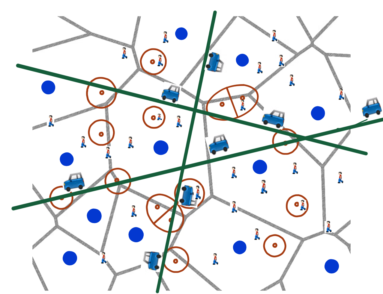
Figure 1: Two-tier heterogeneous network with straight line route system. Statics users are distributed everywhere, whereas mobile users are moving along the routes. The blue circles correspond to macro BSs, and the tiny dots correspond to micro BSs. The regions around the micro BSs correspond to the regions where a micro BS sends the strongest signal. The Voronoi tessellation is generated solely by the process $\Phi_{macro}$. Static users are shown using human symbols, and the mobile users (moving along straight lines) are shown using car symbols.

II-D Downlink Wireless Channel Model

The path-loss at a distance $r$ from a BS is given by $(Ar)^{\beta}$, where $A>0$ and $\beta>2$ are two constants. We ignore all random propagation effects (fading, shadowing) in the channel. Moreover, we focus on the interference limited regime ignoring any thermal noise at the user receivers.

II-E Downlink Service Discipline

Static users are served by the respective BSs in $\Phi$ which are received with the strongest power  . This means that a static user located at $x$ on the plane is served by the station $X_{i}\in\Phi$ which maximizes the value $P_{i}(A|X_{i}-x|)^{-\beta}$, where $P_{i}=P_{macro}$ if $X_{i}\in\Phi_{macro}$ and $P_{i}=P_{micro}$ if $X_{i}\in\Phi_{micro}$. Mobile users are served only by macro BSs in $\Phi_{macro}$, with the choice of the serving station also based on the stronger received power. Due to constant power emitted by macro BSs, this is equivalent to saying that mobile users are served by the respective closest macro BS.

For any micro or macro BS, by its hetnet cell we call the subset of the plane where this station serves static users. For macro BSs, besides their hetnet cells, we consider also macro cells; these are Voronoi cells generated by $\Phi_{macro}$ (ignoring $\Phi_{micro}$), where the macro BSs serve mobile users. Note that the hetnet cells generated by the macro BSs are subsets of the respective macro (Voronoi) cells of these BSs. Also, if $P_{macro}>P_{micro}$ then the hetnet cells of macro BSs are statistically larger than the hetnet cells of the micro BSs. This situation is depicted via Figure 1.

II-F Handoff in the Network

As a MU moves along a line $l\in\mathcal{L}$, it traverses across various macro cells (Voronoi cells generated by $\Phi_{macro}$). On the macro cell boundaries, one macro BS has to hand over the MU to the BS of the neighboring cell; this event is called handoff. We assume in this paper that handoff is always successful (we will discuss in the conclusion how the possibility of handoff failure due to overload in the target cell can be taken care of in our current framework). However, a significant signaling involved during the handoff seriously affects the (downlink) transmission rate during the handoff (see [11, Section $3$]; a MU requires some fixed amount of signaling/overhead communication with the base stations for each handoff). In case of hard handoff, the existing connection to the base station is terminated before the connection to a new base station is established. As a result of this and the signaling overhead, during some short time period for each hard handoff, the mobile user is not able to receive any data from the base station. In case of soft handoff, the mobile user maintains connection to more than one base stations during the handoff period, thereby reducing the spectral efficiency (apart from the throughput loss due to signaling overhead). In order to account for the throughput loss due to handoff in a simplified way, we assume that during handoff, the MU is not able to receive any data from either of the two neighbouring base stations for a constant time $T_{h}$.

Note that MUs do not stop, but keep moving with the usual speed $v$ during the handoff event. Again for simplicity, we assume that the segment of the line $l$ (of length $vT_{h}$) traversed during the handoff period is bisected by the traversed cell boundary.

Note that, if the density of macro BSs is high (and therefore the macro cells sizes are small) with respect to the MU speed $v$, then frequent handoff events have serious detrimental effect on the average downlink data rate of MUs. The reason that we allow only the macro base stations to serve the MUs is to reduce handoff rate by using only large cells for MUs. The goal of the hetnet optimization in $p,P_{macro},P_{micro}$ considered in Section IV is to optimize the performance of the MUs while (at least) preserving the performance of the static users.

II-G Network Equivalence

When optimizing the network design in $p,P_{macro},P_{micro}$, we will consider the following constraint

$$pP_{macro}^{2/\beta}+(1-p)P_{micro}^{2/\beta}=P^{2/\beta}\,,$$ (1)

where $P$ is some given fixed transmission power. Condition (1) ensures that the interference field over $\mathbb{R}^{2}$ generated by the hetnet will have the same marginal distributions as the homogeneous Poisson network of density $\lambda_{BS}$, where each base station transmits at fixed power $P$. For details, see the notion of equivalent homogeneous network as explained in [2, 22]. The equality of the marginal distributions means that all static users experience the same mean service characteristics based on the collection of powers they receive from all macro and micro stations as in the equivalent homogeneous network.

III Performance Evaluation of the Heterogeneous Network

In what follows we shall evaluate the performance of mobile and static users in our hetnet model. We consider mean bit rates of a single, typical SU or MU, the latter accounted for handoff outage events. For both types of users, we also consider the mean throughput, which is defined as the mean peak bit rate divided by the mean number of all (static and mobile) users served by the station serving the typical user. The above performance metrics are subject to network design optimization in Section IV.

III-A Downlink Bit Rate of Mobile Users

Denote by $X^{*}$ the macro BS that is closest to the origin; it is the BS serving the typical MU present at the origin of the plane. Denote by $\mathbf{E}[R_{macro}(0)]$ the mean downlink (Shannon) bit-rate at the origin from $X^{*}$, where $R_{macro}(0)=\log_{2}(1+\text{SIR}_{macro}(0))\,,$ with

$$\text{SIR}_{macro}(0):=\frac{P_{macro}(A|X^{*}|)^{-\beta}}{\sum_{X_{i}\in\Phi,X_{i}\not=X^{*}}P_{i}(A|X_{i}|)^{-\beta}}\,,$$

where $P_{i}=P_{macro}$ if $X_{i}\in\Phi_{macro}$ and $P_{i}=P_{micro}$ if $X_{i}\in\Phi_{micro}$. Observe that MUs treat the power received form micro BSs as noise. We have

$$\mathbf{E}[R_{macro}(0)]=\int_{0}^{\infty}\mathbf{P}\{\text{SIR}_{macro}(0)>(2^{t}-1)\}\,dt$$ (2)

and the distribution of $\text{SIR}_{macro}(0)$ is the subject of the following result.

Theorem 1

For any $\tau>0$, we have:

$$\mathbf{P}(\text{SIR}_{macro}(0)>\tau)$$

$$= \sum_{n=1}^{\lceil{\frac{1}{\tau}}\rceil}(-1)^{n-1}\bigg{(}\frac{\tau}{1-(n-1)\tau}\bigg{)}^{-\frac{2n}{\beta}}\mathcal{J}_{n,\beta}\bigg{(}\frac{\tau}{1-(n-1)\tau}\bigg{)}$$

$$\times\frac{\beta}{2}\times\bigg{(}\frac{2}{\beta\Gamma(1-\frac{2}{\beta})\Gamma(1+\frac{2}{\beta})}\bigg{)}^{n}\bigg{(}1+\frac{(1-p)P_{micro}^{\frac{2}{\beta}}}{pP_{macro}^{\frac{2}{\beta}}}\bigg{)}^{-n}$$

where $\mathcal{J}_{n,\beta}(x)$ is defined in Appendix A, Subsection A (taken from [22, Equation $(16)$] with $x_{1}=x_{2}=\cdots=x_{n}=x$). In particular, for $\tau\geq 1$, we have:

$$\mathbf{P}(\text{SIR}_{macro}(0)>\tau)=\bigg{[}\tau^{\frac{2}{\beta}}\Gamma(1-\frac{2}{\beta})\Gamma(1+\frac{2}{\beta})\bigg{(}1+\frac{(1-p)P_{micro}^{\frac{2}{\beta}}}{pP_{macro}^{\frac{2}{\beta}}}\bigg{)}\bigg{]}^{-1}.$$

Proof:

See Appendix A, Subsection B. ∎

Remark 1

1. Under the equivalent network condition (1), we have:

   $$1+\frac{(1-p)P_{micro}^{\frac{2}{\beta}}}{pP_{macro}^{\frac{2}{\beta}}}=\frac{P^{\frac{2}{\beta}}}{pP_{macro}^{\frac{2}{\beta}}}.$$

2. In case of homogeneous network $P_{macro}=P_{micro}=P$ with only a fraction $p$ of stations potentially serving the origin, the above quantity becomes equal to $1/p$. Then, for $\tau\geq 1$, the probability $\mathbf{P}(\text{SIR}>\tau)$ increases linearly in $p$.

3. Further assuming $p=1$ one obtains the coverage probability in the so called equivalent homogeneous network. It is equal to the coverage probability of the typical static user connecting to the strongest station (macro or micro) in the hetnet, cf. Section III-D.

Remark 2

By the ergodicity of the model, the expectation $\mathbf{E}[R_{macro}(0)]$ is equal almost surely to the sample average data rate along any line of the Poisson line process $\mathcal{L}$. See Appendix A, Subsection C for more explanations.

III-B Accounting for handoff

Note that $\mathbf{E}[R_{macro}(0)]$ does not account for the handoff outage events. An exact way of taking into account this latter phenomenon would require calculating $\mathbf{E}^{0}_{MU}[R_{macro}(0)\mathbf{1}(0\ \text{not in handoff})]$ (where $\mathbf{E}^{0}_{MU}$ is the expectation w.r.t. the Palm probability that a mobile user is located at the origin), which is not amenable to explicit analysis, in particular because of the dependence between $R_{macro}(0)$ and the event $\{0\ \text{not in handoff}\}$. Regarding the handoff probability we have the following bound that involves the intensity

$$\lambda_{c}=\frac{4\sqrt{\lambda_{BS}p}}{\pi}$$

of crossings of a fixed straight line with the boundaries of the macro cells, which are Voronoi cells of $\Phi_{macro}$, cf [25, Equations $5.7.4$ with $m=2$]  .

Lemma 1

$\mathbf{P}_{MU}^{0}\{0\ \text{not in handoff}\}\geq(1-\lambda_{c}vT_{h})$.

Proof:

See Appendix A, Subsection D. ∎

The above bound is meaningful only for $\lambda_{c}vT_{h}$ smaller than 1 and tight when it is close to 0. With the above precautions, for the sake of analytical tractability, we will consider the product $(1-\lambda_{c}vT_{h})\mathbf{E}[R_{macro}(0)]$ as a substitute for the typical MU bit-rate accounted for handoff outage.

III-C Accounting for Other Users — Mean Throughput of MUs

    

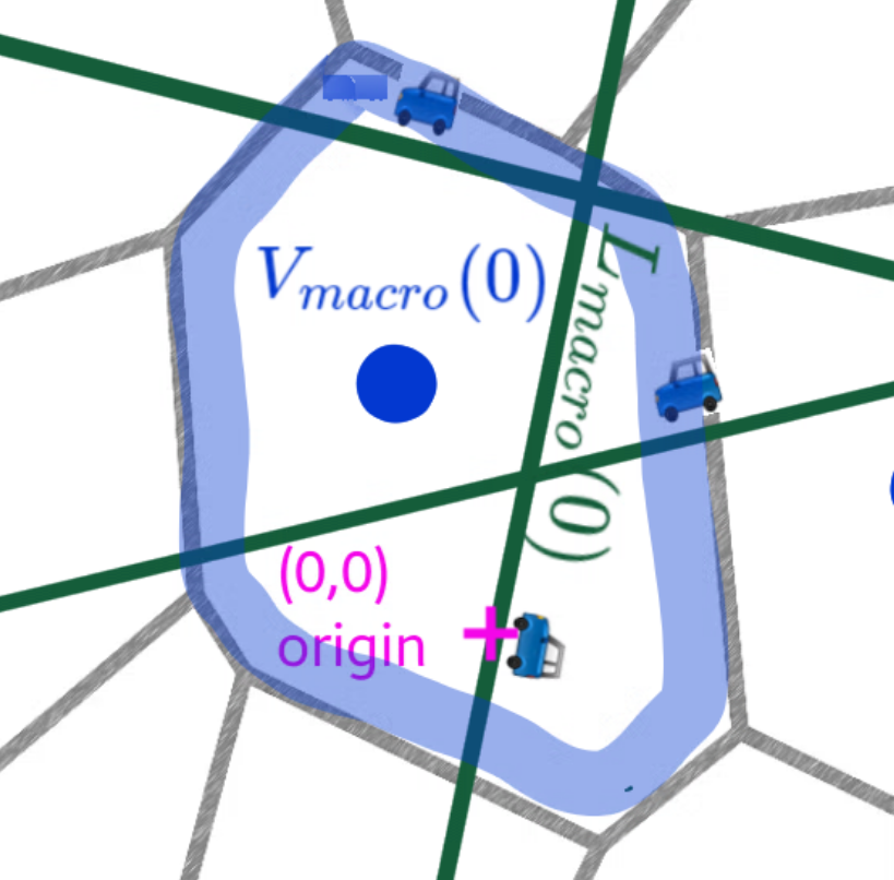
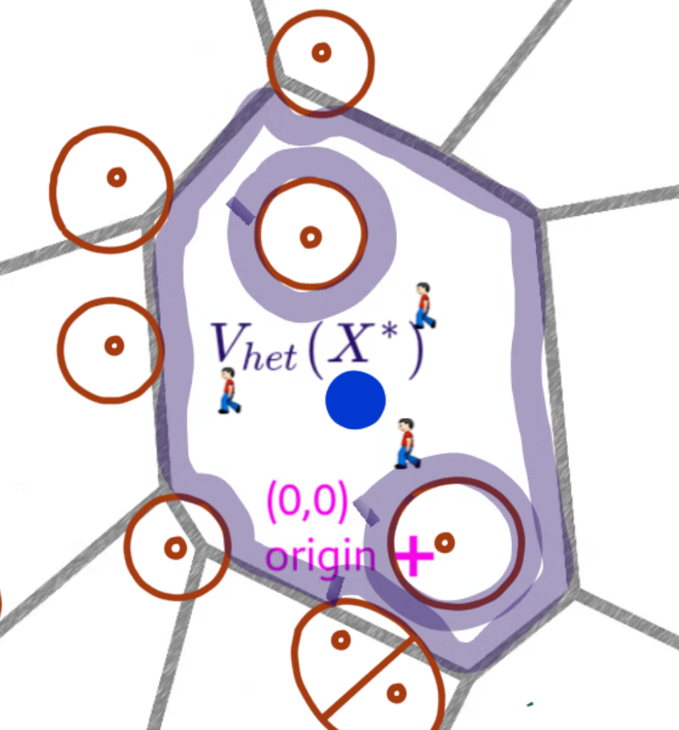
Figure 2: Left: The macro BS $X^{*}$ closest to the origin and its macro-cell, called zero-macro cell. Right: the hetnet cell of $X^{*}$. Note it is not necessarily the hetnet cell covering the origin.

The expression $(1-\lambda_{c}vT_{h})\mathbf{E}[R_{macro}(0)]$ is only the mean bit-rate of a single MU served by $X^{*}$ and does not account for the fact that $X^{*}$ needs to share its resources with other MUs and SUs.

In order to account for the rate sharing with other users, denote by $V_{macro}(0)$ the macro cell of $X^{*}$, and by $|V_{macro}(0)|$ the area of this macro cell. This is the macro cell (generated by $\Phi_{macro}$ alone) covering the origin; cf Figure 2 left. Following standard stochastic geometric terminology we call it zero macro cell. By $\overline{N}_{MU,macro}:=\mathbf{E}^{0}_{MU}[|\mathcal{U}_{mobile}(V_{macro}(0))|]$ we denote the mean number of MUs present in this zero macro cell under the Palm distribution for MUs (i.e., given the typical MU at the origin).

Moreover, let $V_{het}(X^{*})$ be the hetnet cell of $X^{*}$; cf Figure 2 right. Note, it is not necessarily the hetnet cell covering the origin. This is the region where all SUs receive the service from the macro BS $X^{*}$ serving the typical MU present at the origin. Let $\overline{N}_{SU,macro}:=\mathbf{E}^{0}_{MU}[|\mathcal{U}_{static}(V_{het}(X^{*}))|]$ be the mean number of SUs present in the hetnet cell of $X^{*}$ under the Palm distribution for MUs. Note that, by the independence of $\mathcal{U}_{mobile}$, $\mathcal{U}_{static}$, $\Phi_{macro}$ and $\Phi_{micro}$, we can replace $\mathbf{E}^{0}_{MU}$ here simply by $\mathbf{E}$.

We have the following results regarding the two mean number of users.

Theorem 2

The mean number of MUs served by the macro BS serving a typical MU located at the origin is given by: $\overline{N}_{MU,macro}=1+\bigg{(}\frac{1.2802\lambda_{L}}{\lambda_{BS}p}+\frac{3.216}{\pi\sqrt{\lambda_{BS}p}}\bigg{)}\lambda_{MU}$.

Proof:

See Appendix A, Subsection E. ∎

For any two points $(x_{1},x_{2})$ and $(y_{1},y_{2})$ on $\mathbb{R}^{2}$, we define $r_{0}:=(\frac{P_{micro}}{P_{macro}})^{\frac{1}{\beta}}\sqrt{y_{1}^{2}+y_{2}^{2}}$ and $\mathcal{A}((x_{1},x_{2}),(y_{1},y_{2}))$ as the area of the union of two circles with centers at $(x_{1},x_{2})$ and $(y_{1},y_{2})$ and radii $\sqrt{x_{1}^{2}+x_{2}^{2}}$ and $\sqrt{y_{1}^{2}+y_{2}^{2}}$ respectively.

Theorem 3

The mean number of SUs served by the macro BS serving a typical MU located at the origin is given by:

$$\overline{N}_{SU,macro}$$

$$= \lambda_{SU}\lambda_{BS}p\int_{(x_{1},x_{2})\in\mathbb{R}^{2}}\int_{(y_{1},y_{2})\in\mathbb{R}^{2}}$$

$$e^{-\lambda_{BS}p\mathcal{A}((x_{1},x_{2}),(y_{1},y_{2}))-\lambda_{BS}(1-p)\pi r_{0}^{2}}dx_{1}dx_{2}dy_{1}dy_{2}$$

Proof:

See Appendix A, Subsection F. ∎

The two mean number of users allow us to define the mean MU throughput as

$$r_{MU}:=\frac{(1-\lambda_{c}vT_{h})\mathbf{E}[R_{macro}(0)]}{\overline{N}_{SU,macro}+\overline{N}_{MU,macro}}\,.$$ (3)

III-C1 An approximation for $\overline{N}_{SU,macro}$

Since the expression for $\overline{N}_{SU,macro}$ in Theorem 3 is not easy for numerical computation, we approximate it by the expected number of static users served by a typical macro BS in the heterogeneous network $\lambda_{SU}\mathbf{E}_{macro}^{0}[|V_{het}(0)|]$, where $\mathbf{E}_{macro}^{0}$ denotes expectation w.r.t. the Palm probability distribution given that a macro BS is located at the origin. We denote this approximation by $\hat{N}_{SU,macro}$.

Theorem 4

$\hat{N}_{SU,macro}:=\lambda_{SU}\mathbf{E}_{macro}^{0}[|V_{het}(0)|]=\frac{pP_{macro}^{2/\beta}}{pP_{macro}^{2/\beta}+(1-p)P_{micro}^{2/\beta}}\times\frac{\lambda_{SU}}{\lambda_{BS}p}$.

Proof:

See Appendix A, Subsection G. ∎

Theorem 5

$\hat{N}_{SU,macro}\leq\overline{N}_{SU,macro}$.

Proof:

See Appendix A, Subsection H. ∎

III-C2 An upper bound for $\overline{N}_{SU,macro}$

Theorem 6

$\overline{N}_{SU,macro}\leq\frac{1.2802\lambda_{SU}}{\lambda_{BS}p}$.

Proof:

See Appendix A, Subsection I. ∎

III-D Downlink Throughput of Static Users

Following the same line of thought as for MUs, we denote by

$$\mathbf{E}[R_{het}(0)]=\mathbf{E}[\log_{2}(1+\text{SIR}_{het}(0))]$$

the mean downlink bit-rate at the origin from the base station whose hetnet cell is serving the origin;

$$\text{SIR}_{het}(0):=\frac{\max_{i}P_{i}(A|X_{i}|)^{-\beta}}{\sum_{X_{i}\in\Phi}P_{i}(A|X_{i}|)^{-\beta}-\max_{i}P_{i}(A|X_{i}|)^{-\beta}}\,.$$

Here $P_{i}\in\{P_{micro},P_{macro}\}$ is the transmit power from the base station located at $X_{i}\in\Phi$. We consider $\mathbf{E}[R_{het}(0)]$ as the peak bit-rate of the typical SU.

When the condition (1) is satisfied, by the network equivalence principle, cf [2, 22], $\mathbf{E}[R_{het}(0)]=\mathbf{E}[R_{equivalent}(0)]$ where this latter expectation corresponds to $\mathbf{E}[R_{macro}(0)]$ in the one-tier network consisting of only macro BS of intensity $\lambda_{BS}$ and using transmit power $P$. Thus $\mathbf{E}[R_{equivalent}(0)]$ can be evaluated using the expressions in Theorem 1 with $p=1$ and $P_{micro}=P_{macro}=P$, cf. Remark 1.

In order to account for the resource sharing let $V_{het}(0)$ be the zero hetnet cell, i.e., the cell of the (macro or micro) BS that serves a typical SU when present at the origin; cf Figure 3.

Denote by $\overline{N}_{SU,het}:=\mathbf{E}^{0}_{SU}[|\mathcal{U}_{static}(V_{het}(0))|]$ ($|\cdot|$ denotes the cardinality of the set here) the mean number of SUs present in the zero hetnet cell under the Palm distribution for SUs.

Let $\overline{N}_{MU,het}:=\mathbf{E}^{0}_{SU}[|\mathcal{U}_{mobile}(V_{macro}(0))|\mathbf{1}(V_{het}(0)=V_{het}(X^{*}))]$ be the mean number of MUs present in the zero macro cell under the Palm distribution for SUs, provided the BS serving the hetnet cell covering the origin is a macro BS. Note that these are mobile users sharing the service with the typical SU at the origin. Note that, by the independence of $\mathcal{U}_{mobile}$, $\mathcal{U}_{static}$, $\Phi_{macro}$ and $\Phi_{micro}$, we can replace $\mathbf{E}^{0}_{SU}$ here simply by $\mathbf{E}$.

In order to express these two mean numbers denote by $\mathcal{B}((x_{1},x_{2}),(y_{1},y_{2}))$ the area of the union of two circles with centers at $(x_{1},x_{2})$ and $(y_{1},y_{2})$ and radii $(\frac{P_{micro}}{P_{macro}})^{\frac{1}{\beta}}\sqrt{x_{1}^{2}+x_{2}^{2}}$ and $(\frac{P_{micro}}{P_{macro}})^{\frac{1}{\beta}}\sqrt{y_{1}^{2}+y_{2}^{2}}$ respectively. The function $\mathcal{D}((x_{1},x_{2}),(y_{1},y_{2}))$ is defined as the area of the union of two circles with centers at $(x_{1},x_{2})$ and $(y_{1},y_{2})$ and radii $(\frac{P_{macro}}{P_{micro}})^{\frac{1}{\beta}}\sqrt{x_{1}^{2}+x_{2}^{2}}$ and $(\frac{P_{macro}}{P_{micro}})^{\frac{1}{\beta}}\sqrt{y_{1}^{2}+y_{2}^{2}}$ respectively.

Theorem 7

The mean number of SUs served by the (macro or micro) BS serving a typical SU located at the origin is given by:

$$\overline{N}_{SU,het}=1+$$

$$\lambda_{SU}\lambda_{BS}p\int_{(x_{1},x_{2},y_{1},y_{2})\in\mathbb{R}^{4}}e^{-\lambda_{BS}p\mathcal{A}((x_{1},x_{2}),(y_{1},y_{2}))}$$

$$\hskip 24.00005pt\times e^{-\lambda_{BS}(1-p)\mathcal{B}((x_{1},x_{2}),(y_{1},y_{2}))}dx_{1}dx_{2}dy_{1}dy_{2}$$

$$+\lambda_{SU}\lambda_{BS}(1-p)\int_{(x_{1},x_{2},y_{1},y_{2})\in\mathbb{R}^{4}}e^{-\lambda_{BS}(1-p)\mathcal{A}((x_{1},x_{2}),(y_{1},y_{2}))}$$

$$\hskip 24.00005pt\times e^{-\lambda_{BS}p\mathcal{D}((x_{1},x_{2}),(y_{1},y_{2}))}dx_{1}dx_{2}dy_{1}dy_{2}.$$

Proof:

See Appendix A, Subsection J. ∎

Theorem 8

The mean number of MUs served by the same BS serving a typical SU located at the origin is given by:

$$\overline{N}_{MU,het}=\frac{\lambda_{L}\lambda_{MU}}{\lambda_{SU}}\overline{N}_{SU,macro}$$

Proof:

This follows from the mass transport principle, since $\lambda_{SU}\overline{N}_{MU,het}=\lambda_{L}\lambda_{MU}\overline{N}_{SU,macro}$. ∎

We define the mean SU throughput as

$$r_{SU}:=\frac{\mathbf{E}[R_{equivalent}(0)]}{\overline{N}_{SU,het}+\overline{N}_{MU,het}}\,.$$ (4)

III-D1 An approximation for $\overline{N}_{MU,het}$

In order to obtain a computationally simple expression, we define $\hat{N}_{MU,het}:=\mathbf{P}\{V_{het}(0)=V_{het}(X^{*})\}\mathbf{E}[|\mathcal{U}_{mobile}(V_{macro}(0))|]$. This is an approximation to $\overline{N}_{MU,het}$ since the event $\{V_{het}(0)=V_{het}(X^{*})\}$ and the random variable $|\mathcal{U}_{mobile}(V_{macro}(0))|$ are not independent.

Theorem 9

$\hat{N}_{MU,het}=\frac{pP_{macro}^{2/\beta}}{pP_{macro}^{2/\beta}+(1-p)P_{micro}^{2/\beta}}\times\frac{1.2802\lambda_{L}\lambda_{MU}}{\lambda_{BS}p}$.

Proof:

See Appendix A, Subsection K. ∎

III-D2 An approximation for $\overline{N}_{SU,het}$

As an approximation to $\overline{N}_{SU,het}$, we define $\hat{N}_{SU,het}:=1+\mathbf{P}\{V_{het}(0)=V_{het}(X^{*})\}\mathbf{E}_{macro}^{0}[|\mathcal{U}_{static}(V_{het}(0))|]+\mathbf{P}\{V_{het}(0)\neq V_{het}(X^{*})\}\mathbf{E}_{micro}^{0}[|\mathcal{U}_{static}(V_{het}(0))|]$.

Theorem 10

$$\hat{N}_{SU,het} = 1+\bigg{(}\frac{pP_{macro}^{2/\beta}}{pP_{macro}^{2/\beta}+(1-p)P_{micro}^{2/\beta}}\bigg{)}^{2}\frac{\lambda_{SU}}{\lambda_{BS}p}$$ (5)

$$+\bigg{(}\frac{(1-p)P_{micro}^{2/\beta}}{pP_{macro}^{2/\beta}+(1-p)P_{micro}^{2/\beta}}\bigg{)}^{2}\frac{\lambda_{SU}}{\lambda_{BS}(1-p)}$$

Proof:

See Appendix A, Subsection L. ∎

    

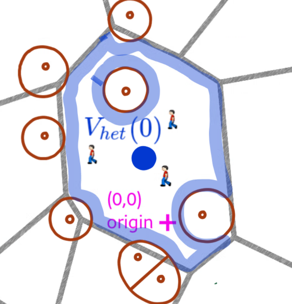
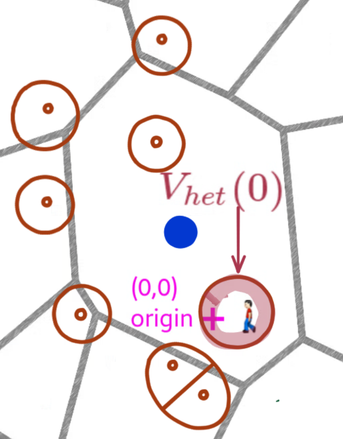
Figure 3: Zero hetnet cell; it may be a macro cell (left) or a micro cell (right). It serves a typical SU at the origin.

IV Optimal Design of the Heterogeneous Network

Let us first consider the network in which all stations transmit with the same power $P_{macro}=P_{micro}=P$. In this homogeneous network, if the density of BSs $\lambda_{BS}$ is high (and hence the cells are small) it might be advantageous to let the mobile users connect only to some fraction $p<1$ of BSs to reduce the frequency of handoffs during which the connection is not assured. Obviously too small $p$ will result is low data rate due to large distance from BSs. Our model allows us to calculate the optimal value of $p$ as a function of mobile speed $v$ and other network parameters. If a heterogeneous structure of the network is allowed, it might be interesting to further optimize jointly the performance of mobile and static users appropriately tuning the powers $P_{macro}$ and $P_{micro}$.

We consider first the optimization of the data rate of mobile users and then optimize the throughput of static and mobile users. The optimal proportion of macro stations and the transmit powers provide a guideline for the design of the heterogeneous network.

IV-A Optimizing Data Rate of Mobile Users

Consider the following optimization of the data rate of mobile users accounted for handoff events (cf Section III-B) within the class of equivalent heterogeneous networks

$$\sup\limits_{\scriptstyle 0\leq p\leq 1,P_{micro},P_{macro}\geq 0\atop\scriptstyle\text{such that~{}\eqref{e.hetnet-equivalence} holds}}\,(1-\lambda_{c}vT_{h})\mathbf{E}[R_{macro}(0)]$$ (6)

for some given $P$ and other model parameters. The above problem needs to be solved numerically since the dependence of the integral (2) for $\mathbf{E}[R_{macro}(0)]$ with the distribution of SIR given in Theorem 1 cannot be analytically evaluated with respect to the optimization parameters.

However, in order to have some insight into the structure of the MU rate optimization let us revisit (6) with $\mathbf{E}[R_{macro}(0)]$ approximated by $\mathbf{E}[R_{macro}(0)\mathbf{1}(\mathrm{SIR}_{macro}(0)>1)]$.  Define the constant

$$C:=(\Gamma(1+2/\beta)\Gamma(1-2/\beta))^{-1}\int_{1}^{\infty}(2^{t}-1)^{-2/\beta}\,dt$$

Then, under constraint (1), $\mathbf{E}[R_{macro}(0)\mathbf{1}(\mathrm{SIR}_{macro}(0)>1)]=Cp(P_{macro}/P_{micor})^{2/\beta}$ and hence

$$(1-\lambda_{c}vT_{h})\mathbf{E}[R_{macro}(0)\mathbf{1}(\mathrm{SIR}_{macro}(0)>1)]=$$

$$(1-4vT_{h}\sqrt{\lambda_{BS}p}/\pi)Cp(P_{macro}/P_{micro})^{2/\beta}.$$ (7)

It is easy to see (calculating the derivative in $p$) that the value of (7) is maximized with $p\in[0,1]$ for $p=p^{*}$, where

$$p^{*}:=\min(1,\pi^{2}/(36v^{2}T_{h}^{2}\lambda_{BS}))\,.$$ (8)

Remark 3

1. Note that the value of $p^{*}$ in (8) does not depend on the power values $P_{macro},P_{micro}$. In case of a homogeneous network these powers are fixed and equal to $P_{macro}=P_{micro}=P$. In this case $p^{*}$ can be interpreted as the optimal fraction of BSs to which MUs should connect so as to optimize their bit-rate. However, it has to be kept in mind that this formula is being used only to provide an intuitive explanation for not using all the base stations to serve the MUs.

2. When a heterogeneous architecture is allowed, the value of (7) with $p=p^{*}$ can be further maximized in $P_{macro}$ under constraint (1). I is easy to see that the optimal choice consists in taking $P_{macro}:=(p^{*})^{\beta/2}P$ and $P_{micro}=0$. This means that using micro BSs is counterproductive from the point of view of the maximization of the bit-rate of MUs. Shutting down micro BSs and increasing appropriately the power of macro BSs (so as to ensure the equivalent service for static users) appears to be an optimal solution. This observation complies with the fact that the micro BSs are meant to provide extra capacity (and not rate-coverage) to the network. Indeed, we shall see in the next section that only a joint optimization of the throughput (which is a capacity metric) of static and mobile users suggest a usage of micro BSs.

IV-B Optimizing User Throughput

We consider now optimization of the user throughput. Our first observation is that if one focuses only on the throughput of mobile users $r_{MU}$ given by (3), i.e. considers

$$\sup\limits_{\scriptstyle 0\leq p\leq 1,P_{micro},P_{macro}\geq 0\atop\scriptstyle\text{such that~{}\eqref{e.hetnet-equivalence} holds}}\,\frac{(1-\lambda_{c}vT_{h})\mathbf{E}[R_{macro}(0)]}{\overline{N}_{SU,macro}+\overline{N}_{MU,macro}}\,,$$ (9)

then, as in the case of MU rate optimization considered in Section IV-A, the optimal solutions consists in taking some $p<1$ when $vT_{h}\sqrt{\lambda_{BS}p}$ too large, do not use micro BSs ($P_{micro}=0$) and adapt appropriately the power of macro BSs (observed numerically). This can be again explained by the observation that micro BSs are meant to provide capacity to static users. When $r_{SU}$ is absent from the optimization then there is no reason to use micro BSs.

This takes us to our ultimate problem of a joint optimization of the throughput of static and mobile users

$$\sup\limits_{\scriptstyle 0\leq p\leq 1,P_{micro},P_{macro}\geq 0\atop\scriptstyle\text{such that~{}\eqref{e.hetnet-equivalence} holds}}\,r_{MU}+\xi r_{SU}$$ (10)

where $r_{MU}$ and $r_{SU}$ is the throughput of mobile and static user given by (3) and (4), respectively, and $\xi$ is a multiplier that captures the emphasis we put on the rate of the typical static user in the objective function.  As we shall see in Section IV-C, if enough emphasis is put on the throughput of static users then the usage of micro stations is advantageous.

Let us denote the optimal solution of (10) by $p^{*}(\xi)$, $P_{micro}^{*}(\xi)$ and $P_{macro}^{*}(\xi)$, and the corresponding optimal rates by $r_{MU}^{*}(\xi)$ and $r_{SU}^{*}(\xi)$.

Lemma 2

$r_{MU}^{*}(\xi)+\xi r_{SU}^{*}(\xi)$ is convex, increasing in $\xi$.

Proof:

See Appendix A, Subsection M. ∎

Lemma 3

$r_{SU}^{*}(\xi)$ is increasing in $\xi$, and $r_{MU}^{*}(\xi)$ is decreasing in $\xi$.

Proof:

See Appendix A, Subsection N. ∎

Problem (10) can be used to solve the following constrained problem:

$$\sup\limits_{\scriptstyle 0\leq p\leq 1,P_{micro},P_{macro}\geq 0\atop\scriptstyle\text{such that~{}\eqref{e.hetnet-equivalence} holds}}\,r_{MU}$$

$$\text{such that }r_{SU}\geq r_{0}$$ (11)

The following standard result tells us how to choose $\xi$.

Theorem 11

If there exists $\xi^{*}\geq 0$ such that, under the optimal solution of (10) with $\xi=\xi^{*}$, the constraint in (11) is met with equality, then that solution is optimal for the constrained problem (11) as well.

IV-C Numerical Results and Insights to the Network Design Problem

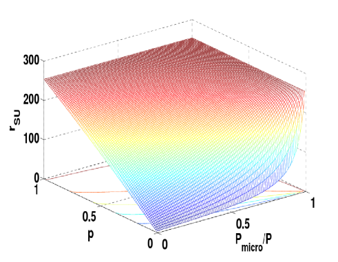
Figure 4: Variation of $r_{SU}$ with $p$ and $\frac{P_{micro}}{P}$ for system parameters chosen in Section IV-C. When $p$ and $P_{micro}$ are both $0$, there are only micro base stations with $0$ transmit power. Hence, all users get zero data rate. This situation is excluded from this plot.

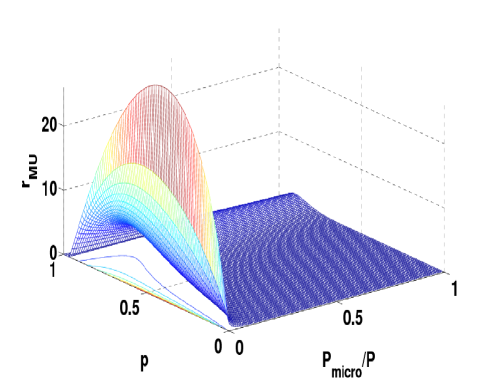
Figure 5: Variation of $r_{MU}$ with $p$ and $\frac{P_{micro}}{P}$ for system parameters chosen in Section IV-C. The situation when $p$ and $P_{micro}$ are both $0$ is not included in the plot.

We consider a networks with $P=1$ unit (the results presented in this section are invariant w.r.t. $P$; the reason is that if we scale the transmit power at each BS by a constant factor, the SIR at any location and the cell structure remain unchanged), $\lambda_{BS}=\frac{1}{2500}/\text{m}^{2}$ (one base station per $50\text{m}\times 50\text{m}$ area), $v=20\text{m}/\text{sec}$ ($72$ kmph), $T_{h}=2$ second (note that, the results in this section will remain unchanged if we vary $v$ and $T_{h}$ while keeping their product constant), $\lambda_{SU}=\frac{1}{400}/\text{m}^{2}$ (one static user per $20\text{m}\times 20\text{m}$ area), $\lambda_{MU}=\frac{1}{20}/\text{m}$ (one MU per $20$ m distance) and $\lambda_{L}=\frac{\sqrt{2}}{50}/\text{m}$ (equivalent to the length of the diagonal in a $50\text{m}\times 50\text{m}$ square).

The variation of $r_{SU}$ and $r_{MU}$ with $p$ and $\frac{P_{micro}}{P}$ are shown in Figure 4 and 5 respectively. Several observations can be made from these plots as discussed below:

• As $p$ or $P_{micro}$ increases, the network becomes more and more homogeneous, and $r_{SU}$ increases.

• As $P_{micro}$ increases for a fixed $p$, the throughput $r_{MU}$ decreases because $P_{macro}$ decreases and interference from micro BSs increases.

• As $p$ increases keeping $P_{micro}$ fixed, $r_{MU}$ first increases and then decreases. Initially $r_{MU}$ increases because more macro BSs are added that can serve the MUs. But beyond certain value of $p$, the throughput loss due to frequent handoff starts dominating, and hence $r_{MU}$ decreases with $p$.

• The performance of MUs is very sensitive to the value of $P_{micro}$; $r_{MU}$ drops rapidly as $P_{micro}$ increases from $0$. Hence, the value of $P_{micro}$ should be small if we want high $r_{MU}$, and the value of $p$ has to be chosen optimally as shown in Figure 4 and 5.

$\xi$	$p^{*}$	$\frac{P_{micro}^{*}}{P}$	$\frac{P_{macro}^{*}}{P}$	$r_{SU}^{*}(\xi)$	$r_{MU}^{*}(\xi)$
				(bits/sec/Hz)	(bits/sec/Hz)
0.001	0.4	0	4.9704	107.0036	33.2543
0.01	0.41	0	4.7602	109.5806	33.2408
0.1	0.5	0	3.3636	132.5683	31.9570
0.2	0.62	0	2.3084	162.6537	27.3609
0.29	0.73	0	1.7345	189.6808	20.6754
0.3	0.9	1	1	253.8792	1.4436
0.4	0.9	1	1	253.8792	1.4436
0.5	0.9	1	1	253.8792	1.4436
1	0.9	1	1	253.8792	1.4436

TABLE I: Effect of $\xi$ on the optimal heterogeneous network design under the equivalent network condition

Now we focus on numerical solution to the problem (10). Let us recall that the optimal solution of (10) is denoted by $p^{*}(\xi)$, $P_{micro}^{*}(\xi)$ and $P_{macro}^{*}(\xi)$, and the corresponding optimal rates are denoted by $r_{MU}^{*}(\xi)$ and $r_{SU}^{*}(\xi)$. From the numerical results in Table I, we observe that $p^{*}<1$, $P_{macro}^{*}>P$ and $P_{micro}^{*}=0$ for small values of $\xi$, whereas $p^{*}<1$, $P_{macro}^{*}=P_{micro}^{*}=P$ above certain value of $\xi$. This is explained by the fact that small $\xi$ puts more weightage on the throughput of mobile users, and hence micro base stations (which cause interference to MU downlink) are shut down, and a fraction of BSs are used as macro BSs with high power. On the other hand, large value of $\xi$ puts more weightage on the throughput of static users, thereby resulting in a homogeneous network design with $P_{macro}^{*}=P_{micro}^{*}=P$. The results also demonstrate that using macro BSs can improve the rate of MUs in practice (which is not intuitive since macro BSs reduce handoff rate, but at the same time a typical MU is co-served with more SUs and MUs, and the macro cell size increases). The interesting part of the observation is that the network should always be homogeneous in both cases; this is a consequence of the sensitivity of $r_{MU}$ with $p$ and $P_{micro}$ as discussed in the previous paragraph. Of course, the optimal design will depend on parameters such as $\lambda_{BS}$, $v$, $T_{h}$, $\lambda_{MU}$ and $\lambda_{L}$, and also the choice of $\xi$; hence, choice of the optimal fraction and power levels of macro and micro base stations will depend on the estimates of user densities and user velocity estimates. The choice will also depend on the physicals constraints of the system designer (e.g., availability and cost for macro and micro BSs, maximum transmit power available at macro BSs etc.) For example, for large $v$, the macro BSs may need very high power, but the commercially available BSs may not be able to meet this power requirement.

From Table I, we can solve the constrained problem (11) by choosing appropriate $\xi^{*}$ as described in Theorem 11.

V Conclusion

In this paper, we have explored the design (or cell planning) of heterogeneous cellular networks to combat throughput loss due to handoff. Analytical results and numerical exploration demonstrate the performance and tradeoffs.

Even though we have solved the basic problem in this paper, there are many possible extensions as well as numerous issues to improve upon: (i) We assumed full interference from all base stations, but it would be of interest to consider the effect of frequency reuse (e.g., in wireless standards such as LTE-A) on the design and resource allocation problems addressed in this paper, (ii) An interesting problem will be cell planning for other models of user mobility such as random waypoint model ([26]), (iii) In practice, there can be multiple possible values of user velocity (generally the network operator will classify user velocities into a discrete set). Hence, a multi-tier network architecture needs to be developed. However, our numerical work has left the open question about the choice of design parameters in such multi-tier networks, since the numerical work with formulation (10) proposes a homogeneous network whereas that formulation cannot achieve all feasible tuples of $(r_{MU},r_{SU})$ (and a solution suboptimal to this formulation has to be adopted), (iv) Extension to the realistic situation where (random) shadowing variation over space modulates the path-loss function is a challenging problem, since this will result in unpredictable behaviour of handoff request generation process due to lack of an accurate statistical characterization of the variation of shadowing over space, (v) Cooperative transmission by multiple base stations to the mobile users can also be explored as a potential solution for throughput loss due to handoff, (vi) Extension to future 5G network models is very challenging, since the association of the mobile users to the densely deployed base stations are supposed to change rapidly over time, resulting in an unprecedented amount of handoff traffic, (vii) In this paper, we have assumed that macro base stations serve SUs and MUs, while micro BSs serve only SUs. There can be other service disciplines, such as macro base stations serving only MUs and micro base stations serving only SUs, or a fraction of macro BSs serving only MUs and some other fraction serving SUs and MUs; performance of such service disciplines needs to be investigated. (viii) The results in this paper do not guarantee a minimum throughput for the users all the time; if a user is located where there is no BS close to it, it will experience poor throughput. A grid-like base station process may be able to solve this issue, but the optimal design procedure of such networks needs to be explored. (ix) A simple way to address the problem of handoff failure due to overload in the target cell would be to multiply the throughput of MUs by the probability that the target macro BS rejects a handoff request (this probability has to be averaged over all macro BSs), and solve the same optimization as in this paper. However, in practice, this probability will be a function of the network design parameters and user densities; hence, the numerical optimization will be more complicated than that solved in this paper. We propose to pursue some of these topics in our future research endeavours.

Arpan Chattopadhyay obtained his B.E. in Electronics and Telecommunication Engineering from Jadavpur University, Kolkata, India in the year 2008, and M.E. and Ph.D in Telecommunication Engineering from Indian Institute of Science, Bangalore, India in the year 2010 and 2015, respectively. He is currently working in INRIA, Paris as a postdoctoral researcher. His research interests include networks, machine learning, information theory and control.

Bartlomiej Blaszczyszyn received his PhD degree and Habilitation qualification in applied mathematics from University of Wrocław (Poland) in 1995 and 2008, respectively. He is now a Senior Researcher at Inria (France), and a member of the Computer Science Department of Ecole Normale Supérieure in Paris. His professional interests are in applied probability, in particular in stochastic modeling and performance evaluation of communication networks. He coauthored several publications on this subject in major international journals and conferences, as well as a two-volume book on Stochastic Geometry and Wireless Networks NoW Publishers, jointly with F. Baccelli.

Eitan Altman received the B.Sc. degree in electrical engineering (1984), the B.A. degree in physics (1984) and the Ph.D. degree in electrical engineering (1990), all from the Technion-Israel Institute, Haifa. In (1990) he further received his B.Mus. degree in music composition in Tel-Aviv University. Since 1990, he has been with INRIA (National research institute in informatics and control) in Sophia-Antipolis, France. His current research interests include performance evaluation and control of telecommunication networks and in particular congestion control, wireless communications and networking games. He is in the editorial board of several scientific journals: JEDC, COMNET, DEDS and WICON. He has been the (co)chairman of the program committee of several international conferences and workshops on game theory, networking games and mobile networks.

Appendix A

A Expression for $\mathcal{J}_{n,\beta}(\cdot)$ function

The function $\mathcal{J}_{n,\beta}(x_{1},x_{2},\cdots,x_{n})$ is defined as follows:

$$\frac{(1+\sum_{j=1}^{n}x_{j})}{n}\int_{[0,1]^{n-1}}\frac{\Pi_{i=1}^{n-1}v_{i}^{i(\frac{2}{\beta}+1)-1}(1-v_{i})^{\frac{2}{\beta}}}{\Pi_{i=1}^{n}(x_{i}+\eta_{i})}dv_{1}dv_{2}\ldots dv_{n-1}$$

where

$$\eta_{1} = v_{1}v_{2}\ldots v_{n-1}$$

$$\eta_{2} = (1-v_{1})v_{2}\ldots v_{n-1}$$

$$\eta_{3} = (1-v_{2})v_{3}\ldots v_{n-1}$$

$$\cdots$$

$$\eta_{n} = 1-v_{n-1}$$

The function $\mathcal{J}_{n,\beta}(x)$ is calculated by substituting $x_{1}=x_{2}=\cdots=x_{n}=x$ in the expression for $\mathcal{J}_{n,\beta}(x_{1},x_{2},\cdots,x_{n})$.

B Proof of Theorem 1

Denote $\text{SIR}=\text{SIR}_{macro}(0)$ and denote the interference at the origin by the base stations belonging to $\Phi_{micro}$ by $I_{micro}$. For a given realization of $I_{micro}$, using [22, Corollary $19$]), we can write that, $\mathbf{P}(\text{SIR}>\tau|I_{micro})=\sum_{n=1}^{\lceil{\frac{1}{\tau}}\rceil}(-1)^{n-1}\tau_{n}^{-\frac{2n}{\beta}}\mathcal{J}_{n,\beta}(\tau_{n})\mathcal{I}_{n,\beta}(I_{micro}a^{-\frac{\beta}{2}})$, where $\tau_{n}:=\frac{\tau}{1-(n-1)\tau}$, $a=\frac{\pi\lambda_{BS}pP_{macro}^{\frac{2}{\beta}}}{A^{2}}$, and the function $\mathcal{I}_{n,\beta}(\cdot)$ is defined in [22, Equation $(13)$]. For completeness, we provide the expression $\mathcal{I}_{n,\beta}(x):=\frac{2^{n}\int_{0}^{\infty}u^{2n-1}e^{-u^{2}-u^{\beta}x\Gamma(1-2/\beta)^{-\beta/2}}du}{\beta^{n-1}(n-1)!\Gamma(1-2/\beta)^{n}\Gamma(1+2/\beta)^{n}}$.

Unconditioning $\mathcal{I}_{n,\beta}(I_{micro}a^{-\frac{\beta}{2}})$ over $I_{micro}$, we obtain:

$$\mathbf{E}[\mathcal{I}_{n,\beta}(I_{micro}a^{-\frac{\beta}{2}})]$$

$$=\bigg{(}\beta^{n-1}(n-1)!\bigg{)}^{-1}\bigg{(}\frac{2}{\Gamma(1-\frac{2}{\beta})\Gamma(1+\frac{2}{\beta})}\bigg{)}^{n}$$

$$\times\int_{0}^{\infty}u^{2n-1}e^{-u^{2}}\mathbf{E}[e^{-I_{micro}a^{-\frac{\beta}{2}}u^{\beta}\Gamma(1-\frac{2}{\beta})^{-\frac{\beta}{2}}}]du.$$

From [27, Equation $(3.3)$], we can write the Laplace transform

$$\mathbf{E}[e^{-I_{micro}a^{-\frac{\beta}{2}}u^{\beta}\Gamma(1-\frac{2}{\beta})^{-\frac{\beta}{2}}}] =\mathcal{L}_{I_{micro}}(a^{-\frac{\beta}{2}}u^{\beta}\Gamma(1-\frac{2}{\beta})^{-\frac{\beta}{2}})$$

$$=e^{-\lambda_{BS}(1-p)A^{-2}a^{-1}u^{2}\pi P_{micro}^{\frac{2}{\beta}}}$$

$$=e^{-u^{2}(1-p)/p(P_{micro}/P_{macro})^{\frac{2}{\beta}}}.$$

Putting this into the expression of $\mathbf{P}(\text{SIR}>\tau)$ we obtain

$$\mathbf{P}(\text{SIR}>\tau)$$

$$= \sum_{n=1}^{\lceil{\frac{1}{\tau}}\rceil}(-1)^{n-1}\tau_{n}^{-\frac{2n}{\beta}}\mathcal{J}_{n,\beta}(\tau_{n})\times\bigg{(}\beta^{n-1}(n-1)!\bigg{)}^{-1}$$

$$\times\bigg{(}\frac{2}{\Gamma(1-\frac{2}{\beta})\Gamma(1+\frac{2}{\beta})}\bigg{)}^{n}\times\int_{0}^{\infty}u^{2n-1}e^{-u^{2}\bigg{(}1+\frac{(1-p)P_{micro}^{\frac{2}{\beta}}}{pP_{macro}^{\frac{2}{\beta}}}\bigg{)}}du$$

Substituting $v:=u^{2}\bigg{(}1+\frac{(1-p)P_{micro}^{\frac{2}{\beta}}}{pP_{macro}^{\frac{2}{\beta}}}\bigg{)}$ in the above integral and simplifying it further, we prove the lemma. It might be also useful to observe that $2/(\Gamma(1-\frac{2}{\beta})\Gamma(1+\frac{2}{\beta})=\beta/\pi\sin(2\pi/\beta+\pi)$

C Proof of Remark 2

Consider a given directed line $l$ on the plane. Note that the couple $(\Phi_{macro},\Phi_{micro})$ is ergodic (by [28, Proposition $2.6$]) and the $\sigma$-field $\sigma(\Phi_{macro},\Phi_{micro})$ is countably generated. Hence, by [28, Proposition $2.7$], the sample average data rate (average of $R_{macro}(x)$ taken over all points $x$ along line $l$), exists and is almost surely equal to a constant $c_{l}$ for all, except for at most countably many number of lines $l$, with $c_{l}=\mathbf{E}[R_{macro}(x_{l})]$ for arbitrary $x_{l}\in l$. Since the couple $(\Phi_{macro},\Phi_{micro})$ is translation invariant $\mathbf{E}[R_{macro}(x_{l})]=\mathbf{E}[R_{macro}(0)]$. Finally, probability that the Poisson line process $\mathcal{L}$ places some of its lines in the at most countable subset of lines $l$ is null.

D Proof of Lemma 1

Recall that $\lambda_{c}$ is the density of handoffs (macro cell boundary crossings) on every line of $\mathcal{L}$. Observe that $vT_{h}$ is the length of the segment corresponding to each handoff event. If the segments corresponding to different handoffs on a given line were disjoint the fraction of the line where mobiles are not in handoff would be equal to $1-\lambda_{c}vT_{h}$. The inequality results from the fact that two different handoff events may have overlapping segments on the line, or, in other words, that (in case of crossing small cells) a MU may not recover from the previous handoff before going into the next one.

E Proof of Theorem 2

Under $\mathbf{E}_{MU}^{0}$ the typical MU is located at the origin, while other MUs form a Poisson process of intensity $\lambda_{MU}$ on lines of the original, independent $\mathcal{L}$ appended with one extra line, crossing the origin and independently, uniformly oriented. This is the line along which moves the typical user. Denote by $L_{macro}(0)$ the intersection of this extra line with $V_{macro}(0)$ and by $|V_{macro}(0)|$ and $|L_{macro}(0)|$ the respective area and length. Knowing that the expected total length of intersection of $\mathcal{L}$ with any given set is equal to $\lambda_{L}$ times the surface of this set we have:

$$\overline{N}_{MU,macro}=1+(\lambda_{L}\mathbf{E}[|V_{macro}(0)|+\mathbf{E}_{MU}^{0}[|L_{macro}(0)|])\lambda_{MU},$$ (12)

where we replaced $\mathbf{E}_{MU}^{0}$[…] by $\mathbf{E}[...]$ in the first term due to independence of $\mathcal{L}$ and $\Phi$. By the inverse formula of Palm calculus, cf. [29, Theorem 4.1 and Corollary 4.4], we have $\mathbf{E}[|V_{macro}(0)|]=\frac{\mathbf{E}_{macro}^{0}[|V_{macro}(0)|^{2}]}{\mathbf{E}_{macro}^{0}[|V_{macro}(0)|]},$ where $\mathbf{E}_{macro}^{0}$ corresponds to Palm distribution for $\Phi_{macro}$ (i.e. given a macro BS at the origin). Now, $\mathbf{E}_{macro}^{0}[|V_{macro}(0)|]=1/(\lambda_{BS}p)$, (cf  [29, Corollary 4.3]) and the variance $\mathbf{Var}_{macro}^{0}(|V_{macro}(0)|)=\frac{0.2802}{(\lambda_{BS}p)^{2}}$ (cf [24, Table $9.5$]) Hence, $\mathbf{E}_{macro}^{0}[|V_{macro}(0)|^{2}]=\mathbf{Var}_{macro}^{0}(|V_{macro}(0)|)+(\mathbf{E}_{macro}^{0}[|V_{macro}(0)|]^{2}=\frac{1.2802}{(\lambda_{BS}p)^{2}}$ and consequently $\mathbf{E}[|V_{macro}(0)|]=\frac{1.2802}{\lambda_{BS}p}$.

Regarding the length of $L_{macro}(0)$ under $\mathbf{E}_{MU}^{0}$, we can observe that it has the same distribution as the length of the interval $\tilde{L}(0)$ between two consecutive handoffs (crossings of the macro cell boundary) of, say, $x$ axis, which covers the origin. $\tilde{L}(0)$ is hence the zero interval (the one covering the origin) of the point process of macro cell boundary crossings with the $x$ axis. This process has intensity $\lambda_{c}=\frac{4\sqrt{\lambda_{BS}p}}{\pi}$ cf [25, Equations $5.7.4$ with $m=2$]. Using the same inverse formula (this time in one dimension) we obtain:

$$\mathbf{E}_{MU}^{0}[|L_{macro}(0)|]=\mathbf{E}[|\tilde{L}(0)|]=\lambda_{c}\mathbf{E}_{cross}^{0}[|\tilde{L}(0)|^{2}]\,$$

where $\mathbf{E}_{cross}^{0}$ corresponds to the Palm probability of the point process of the macro cell boundary crossings by the horizontal $x$ axis. By [25, Table $5.7.2$], $\mathbf{E}_{cross}^{0}[|\tilde{L}_{macro}(0)|]^{2}=\frac{0.804}{\lambda_{BS}p}$. Hence,

$$\mathbf{E}_{MU}^{0}[|L_{macro}(0|]=\frac{0.804\times 4}{\pi\times\sqrt{\lambda_{BS}p}}=\frac{3.216}{\pi\sqrt{\lambda_{BS}p}}.$$

Plugging in the expression (12) we prove the theorem.

F Proof of Theorem 3

Let $\mathbf{E}_{macro}^{0}$ denote expectation w.r.t. the Palm probability distribution $\mathbf{P}_{macro}^{0}$ (probability given that a macro BS is located at the origin). Similarly as in the proof of Theorem 2:

$$\overline{N}_{SU,macro} = \lambda_{SU}\mathbf{E}[|V_{het}(X^{*})|]$$ (13)

$$= \lambda_{SU}\frac{\mathbf{E}_{macro}^{0}[|V_{het}(0)|\times|V_{macro}(0)|]}{\mathbf{E}_{macro}^{0}[|V_{macro}(0)|]}$$

$$= \lambda_{SU}\lambda_{BS}p\mathbf{E}_{macro}^{0}[|V_{het}(0)|\times|V_{macro}(0)|]$$

where the first equality is by the independence between $\mathcal{U}_{static}$ and $\Phi$ and the second by the inverse formula of Palm calculus. Now,

$$\mathbf{E}_{macro}^{0}[|V_{het}(0)|\times|V_{macro}(0)|]$$ (14)

$$= \mathbf{E}_{macro}^{0}\bigg{(}\int_{(x_{1},x_{2})\in\mathbb{R}^{2}}\mathbf{1}\{(x_{1},x_{2})\in V_{macro}(0)\}dx_{1}dx_{2}$$

$$\times\int_{(y_{1},y_{2})\in\mathbb{R}^{2}}\mathbf{1}\{(y_{1},y_{2})\in V_{het}(0)\}dy_{1}dy_{2}\bigg{)}$$

$$= \mathbf{E}_{macro}^{0}\bigg{(}\int_{(x_{1},x_{2})}\int_{(y_{1},y_{2})}\mathbf{1}\{(x_{1},x_{2})\in V_{macro}(0),$$

$$\hskip 40.00008pt(y_{1},y_{2})\in V_{het}(0)\}dx_{1}dx_{2}dy_{1}dy_{2}\bigg{)}$$

$$= \int_{(x_{1},x_{2})}\int_{(y_{1},y_{2})}\mathbf{P}_{macro}^{0}\{(x_{1},x_{2})\in V_{macro}(0),$$

$$\hskip 40.00008pt(y_{1},y_{2})\in V_{het}(0)\}dx_{1}dx_{2}dy_{1}dy_{2}$$

Given that there is a macro BS at the origin, $(x_{1},x_{2})\in V_{macro}(0)$ and $(y_{1},y_{2})\in V_{het}(0)$ if and only if these three conditions are satisfied: (i) there is no other macro BS in a circle centered at $(x_{1},x_{2})$ and having radius $\sqrt{x_{1}^{2}+x_{2}^{2}}$, (ii) there is no other macro BS in a circle centered at $(y_{1},y_{2})$ and having radius $\sqrt{y_{1}^{2}+y_{2}^{2}}$, and (iii) there is no other micro BS inside a circle centered at $(y_{1},y_{2})$ and having radius $r_{0}$ where $P_{macro}(\sqrt{y_{1}^{2}+y_{2}^{2}})^{-\beta}=P_{micro}r_{0}^{-\beta}$, i.e., $r_{0}=(\frac{P_{micro}}{P_{macro}})^{\frac{1}{\beta}}\sqrt{y_{1}^{2}+y_{2}^{2}}$.

Hence,

$$\mathbf{P}_{macro}^{0}\{(x_{1},x_{2})\in V_{macro}(0),(y_{1},y_{2})\in V_{het}(0)\}$$

$$=e^{-\lambda_{BS}p\mathcal{A}((x_{1},x_{2}),(y_{1},y_{2}))-\lambda_{BS}(1-p)\pi r_{0}^{2}}\,,$$

where $r_{0}=(\frac{P_{micro}}{P_{macro}})^{\frac{1}{\beta}}\sqrt{y_{1}^{2}+y_{2}^{2}}$. This, combined with (13) and (14), proves the theorem.

G Proof of Theorem 4

Let us assume that the macro BS closest to the origin is located at a distance $r$ from the origin. Then, the origin will be served by the macro BS if and only if there is no micro BS in a circle centered at origin with radius $R$, where $P_{micro}R^{-\beta}=P_{macro}r^{-\beta}$, i.e., $R=(\frac{P_{micro}}{P_{macro}})^{1/\beta}r$. The probability that the nearest macro BS to the origin is located at a distance between $r$ and $r+dr$ is given by $f(r)dr$ where $f(r)=e^{-\lambda_{BS}p\pi r^{2}}\lambda_{BS}p\times 2\pi r$. Hence, the probability that a static user located at the origin is served by a macro BS is given by $\int_{0}^{\infty}e^{-\lambda_{BS}(1-p)\pi(P_{micro}/P_{macro})^{2/\beta}r^{2}}f(r)dr$, which, after simplification, yields that the probability that a typical static user located at the origin is served by a macro BS is given by $\frac{pP_{macro}^{2/\beta}}{pP_{macro}^{2/\beta}+(1-p)P_{micro}^{2/\beta}}$. This is also the fraction of area over $\mathbb{R}^{2}$ where SUs are served by macro BSs.

Now, by the inverse formula of Palm calculus, $\mathbf{E}_{macro}^{0}[|V_{het}(0)|]=\frac{pP_{macro}^{2/\beta}}{pP_{macro}^{2/\beta}+(1-p)P_{micro}^{2/\beta}}\times\frac{1}{\lambda_{BS}p}$, from which the proof follows.

H Proof of Theorem 5

Let us recall the expression for $\overline{N}_{SU,macro}$ from Theorem 3. Note that, $\mathcal{A}((x_{1},x_{2}),(y_{1},y_{2}))\leq\pi(x_{1}^{2}+x_{2}^{2})+\pi(y_{1}^{2}+y_{2}^{2})$. Hence,

$$\overline{N}_{SU,macro}$$

$$\geq \lambda_{SU}\lambda_{BS}p\int_{(x_{1},x_{2})\in\mathbb{R}^{2}}\int_{(y_{1},y_{2})\in\mathbb{R}^{2}}$$

$$e^{-\lambda_{BS}p\pi(x_{1}^{2}+x_{2}^{2})-\lambda_{BS}p\pi(y_{1}^{2}+y_{2}^{2})-\lambda_{BS}(1-p)\pi r_{0}^{2}}$$

$$dx_{1}dx_{2}dy_{1}dy_{2}$$

Now, $\int_{(x_{1},x_{2})\in\mathbb{R}^{2}}e^{-\lambda_{BS}p\pi(x_{1}^{2}+x_{2}^{2})}dx_{1}dx_{2}=\mathbf{E}_{macro}^{0}(|V_{macro}(0)|)=\frac{1}{\lambda_{BS}p}$ and $\int_{(y_{1},y_{2})\in\mathbb{R}^{2}}e^{-\lambda_{BS}p\pi(y_{1}^{2}+y_{2}^{2})-\lambda_{BS}(1-p)\pi r_{0}^{2}}dy_{1}dy_{2}=\mathbf{E}_{macro}^{0}(|V_{het}(0)|)$. Hence, $\overline{N}_{SU,macro}\geq\lambda_{SU}\mathbf{E}_{macro}^{0}(|V_{het}(0)|):=\hat{N}_{SU,macro}$.

I Proof of Theorem 6

Note that, $\overline{N}_{SU,macro}=\lambda_{SU}\mathbf{E}_{MU}^{0}[|V_{het}(X^{*})|]$. But $V_{het}(X^{*})$ is a subset of macro cell $V_{macro}(0)$ containing the origin, and $\mathbf{E}_{MU}^{0}[|V_{macro}(0)|]=\mathbf{E}[|V_{macro}(0)|]=\frac{1.2802}{\lambda_{BS}p}$ (as shown in the proof of Theorem 2). Hence, $\overline{N}_{SU,macro}\leq\frac{1.2802\lambda_{SU}}{\lambda_{BS}p}$.

J Proof of Theorem 7

We consider now the typical SU located at the origin under $\mathbf{E}_{SU}^{0}$. Using the similar arguments as in the proof of Theorem 3, we obtain:

$$\overline{N}_{SU,het} = 1+\lambda_{SU}\mathbf{E}[|V_{het}(0)|]$$ (15)

$$= 1+\lambda_{SU}\frac{\mathbf{E}_{het}^{0}[|V_{het}(0)|^{2}]}{\mathbf{E}_{het}^{0}[|V_{het}(0)|]}\,,$$

where $\mathbf{E}_{het}^{0}$ denotes the expectation under the Palm probability given that there is one (macro or micro) BS at the origin. Let $\mathbf{E}_{macro}^{0}$ (resp., $\mathbf{E}_{micro}^{0}$) be the expectation under the Palm probability distribution given that there is one macro (resp., micro) BS at the origin. Note that, the fraction of the macro base stations is $p$, and the rest of base stations are micro base stations. Using this fact and using similar arguments as in the proof of Theorem 3, we can write:

$$\mathbf{E}_{het}^{0}[|V_{het}(0)|^{2}]$$ (16)

$$= p\int_{(x_{1},x_{2})\in\mathbb{R}^{2}}\int_{(y_{1},y_{2})\in\mathbb{R}^{2}}$$

$$\mathbf{P}_{macro}^{0}\{(x_{1},x_{2})\in V_{het}(0),(y_{1},y_{2})\in V_{het}(0)\}dx_{1}dx_{2}dy_{1}dy_{2}$$

$$+(1-p)\int_{(x_{1},x_{2})\in\mathbb{R}^{2}}\int_{(y_{1},y_{2})\in\mathbb{R}^{2}}$$

$$\mathbf{P}_{micro}^{0}\{(x_{1},x_{2})\in V_{het}(0),(y_{1},y_{2})\in V_{het}(0)\}dx_{1}dx_{2}dy_{1}dy_{2}$$

$$= p\int_{(x_{1},x_{2})\in\mathbb{R}^{2}}\int_{(y_{1},y_{2})\in\mathbb{R}^{2}}e^{-\lambda_{BS}p\mathcal{A}((x_{1},x_{2}),(y_{1},y_{2}))}$$

$$e^{-\lambda_{BS}(1-p)\mathcal{B}((x_{1},x_{2}),(y_{1},y_{2}))}dx_{1}dx_{2}dy_{1}dy_{2}$$

$$+(1-p)\int_{(x_{1},x_{2})\in\mathbb{R}^{2}}\int_{(y_{1},y_{2})\in\mathbb{R}^{2}}e^{-\lambda_{BS}(1-p)\mathcal{A}((x_{1},x_{2}),(y_{1},y_{2}))}$$

$$e^{-\lambda_{BS}p\mathcal{D}((x_{1},x_{2}),(y_{1},y_{2}))}dx_{1}dx_{2}dy_{1}dy_{2}$$

Now, note that $\mathbf{E}_{het}^{0}[|V_{het}(0)|]=1/\lambda_{BS}$. This, combined with (15) and (16) proves the theorem.

K Proof of Theorem 9

As in the proof of Theorem 4, $\mathbf{P}\{V_{het}(X^{*})=V_{het}(0)\}=\frac{pP_{macro}^{2/\beta}}{pP_{macro}^{2/\beta}+(1-p)P_{micro}^{2/\beta}}$. The mean volume of the zero macro cell (the macro cell containing the origin) is $\mathbf{E}(|V_{macro}(0)|)=\frac{1.2802}{\lambda_{BS}p}$ as in the proof of Theorem 2, and $\mathbf{E}(|\mathcal{U}_{mobile}(V_{macro}(0))|)=\lambda_{MU}\lambda_{L}\mathbf{E}(|V_{macro}(0)|)$. Hence, the proof follows.

L Proof of Theorem 10

As in the proof of Theorem 4, $\mathbf{P}\{V_{het}(X^{*})=V_{het}(0)\}=\frac{pP_{macro}^{2/\beta}}{pP_{macro}^{2/\beta}+(1-p)P_{micro}^{2/\beta}}$. Now, $\mathbf{P}\{V_{het}(X^{*})\neq V_{het}(0)\}=1-\mathbf{P}\{V_{het}(X^{*})=V_{het}(0)\}$.

Similar to the proof of Theorem 4, the mean area of a hetnet cell served by a typical macro BS is given by $\mathbf{E}_{macro}^{0}[|V_{het}(0)|]=\frac{pP_{macro}^{2/\beta}}{pP_{macro}^{2/\beta}+(1-p)P_{micro}^{2/\beta}}\times\frac{1}{\lambda_{BS}p}$, and similarly $\mathbf{E}_{micro}^{0}[|V_{het}(0)|]=\frac{(1-p)P_{micro}^{2/\beta}}{pP_{macro}^{2/\beta}+(1-p)P_{micro}^{2/\beta}}\times\frac{1}{\lambda_{BS}(1-p)}$.

Combining the above results, we prove the theorem.

M Proof of Lemma 2

Note that, for given values of $p$, $P_{micro}$ and $P_{macro}$, the function $(r_{MU}+\xi r_{SU})$ is an affine, increasing function of $\xi$. This proves the lemma since pointwise supremum of affine, increasing functions is convex, increasing.

N Proof of Lemma 3

Consider any $\kappa>0$. By optimality of $p^{*}(\xi)$, $P_{micro}^{*}(\xi)$ and $P_{macro}^{*}(\xi)$, we obtain:

$$r_{MU}(p^{*}(\xi),P_{micro}^{*}(\xi),P_{macro}^{*}(\xi))$$

$$+\xi r_{SU}(p^{*}(\xi),P_{micro}^{*}(\xi),P_{macro}^{*}(\xi))$$

$$\geq r_{MU}(p^{*}(\xi+\kappa),P_{micro}^{*}(\xi+\kappa),P_{macro}^{*}(\xi+\kappa))$$

$$+\xi r_{SU}(p^{*}(\xi+\kappa),P_{micro}^{*}(\xi+\kappa),P_{macro}^{*}(\xi+\kappa))$$

and

$$r_{MU}(p^{*}(\xi+\kappa),P_{micro}^{*}(\xi+\kappa),P_{macro}^{*}(\xi+\kappa))$$

$$+(\xi+\kappa)r_{SU}(p^{*}(\xi+\kappa),P_{micro}^{*}(\xi+\kappa),P_{macro}^{*}(\xi+\kappa))$$

$$\geq r_{MU}(p^{*}(\xi),P_{micro}^{*}(\xi),P_{macro}^{*}(\xi))$$

$$+(\xi+\kappa)r_{SU}(p^{*}(\xi),P_{micro}^{*}(\xi),P_{macro}^{*}(\xi))$$

Adding the above inequalities and cancelling common terms, we obtain $r_{SU}(p^{*}(\xi+\kappa),P_{micro}^{*}(\xi+\kappa),P_{macro}^{*}(\xi+\kappa))\geq r_{SU}(p^{*}(\xi),P_{micro}^{*}(\xi),P_{macro}^{*}(\xi))$, i.e., $r_{SU}^{*}(\xi)$ is increasing in $\xi$. We can prove the other part in a similar way.

References

- [1] H.S. Dhillon, R.K. Ganti, F. Baccelli, and J.G. Andrews. Modeling and analysis of K-tier downlink heterogeneous cellular networks. Selected Areas in Communications, IEEE Journal on, 30(3):550–560, april 2012.
- [2] B. Błaszczyszyn and Holger Paul Keeler. Equivalence and comparison of heterogeneous cellular networks. In Proc. of PIMRC/WDN-CN, 2013.
- [3] J. Andrews, H. Claussen, M. Dohler, S. Rangan, and M. Reed. Femtocells: Past, present and future. IEEE Journal on Selected Areas in Communications, 30(3):497–508, 2012.
- [4] V. Pauli, J. Diego Naranjo, and E. Seidel. Heterogeneous LTE networks and inter-cell interference coordination. http://nomor.de/home/technology/white-papers/lte-hetnet-and-icic, 2010. Nomor Research White Paper.
- [5] O. Stanze and A. Weber. Heterogeneous networks with lte-advanced technologies. Bell Labs Technical Journal, 18(1):41—58, 2013.
- [6] T. Nakamura, S. Nagata, A. Benjebbour, Y. Kishiyama, T. Hai, S. Xiaodong, Y. Ning, and L. Nan. Trends in small cell enhancements in lte advanced. IEEE Communications Magazine, 51(2):98–105, 2013.
- [7] H. Ishii, Y. Kishiyama, and H. Takahashi. A novel architecture for lte-b c-plane/u-plane split and phantom cell concept. In IEEE Globecom Workshops, pages 624–630, 2012.
- [8] T. Camp, J. Boleng, and V. Davies. A survey of mobility models for ad hoc network research. Wireless Communication and Mobile Computing (WCMC): Special Issue on Mobile Ad Hoc Networking: Research, Trends and Applications, 2:483–502, 2002.
- [9] E. Halepovic and C. Williamson. Characterizing and modeling user mobility in a cellular data network. In Proc. 2nd ACM international workshop on Performance evaluation of wireless ad hoc, sensor and ubiquitous networks, pages 71—78. ACM, 2005.
- [10] I. F. Akyildiz, J. McNair, J. S. Ho, H. Uzunalioglu, and W. Wang. Mobility management in next-generation wireless systems. Proceedings of the IEEE, 87(8):1347–1384, August 1999.
- [11] V. Kavitha, S. Ramanath, and E. Altman. Spatial queueing for analysis, design and dimensioning of picocell networks with mobile users. Performance Evaluation, 68:710–727, 2011.
- [12] Z. Ye, L.K. Law, S.V. Krishnamurthy, Z. Xu, S. Dhirakaosal, S.K. Tripathi, and M. Molle. Predictive channel reservation for handoff prioritization in wireless cellular networks. Computer Networks, 51(3):798–822, 2007.
- [13] M. Grossglauser and D.N.C. Tse. Mobility increases the capacity of ad hoc wireless networks. IEEE/ACM Transactions on Networking, 10(4):477–486, 2002.
- [14] N. Bansal and Z. Liu. Capacity, delay and mobility in wireless ad-hoc networks. In Twenty-Second Annual Joint Conference of the IEEE Computer and Communications (INFOCOM), Vol. 2, pages 1553—1563. IEEE, 2003.
- [15] T. Bonald, S. Borst, N. Hegde, M. Jonckheere, and A. Proutiere. Flow-level performance and capacity of wireless networks with user mobility. Queueing Systems: Theory and Applications, 63:131–164, 2009.
- [16] T. Bonald, S.C. Borst, and A. Proutiere. How mobility impacts the flow-level performance of wireless data systems. In Twenty-third Annual Joint Conference of the IEEE Computer and Communications Societies (INFOCOM), Vol. 3, pages 1872—1881. IEEE, 2004.
- [17] S. Borst, A. Proutiere, and N. Hegde. Capacity of wireless data networks with intra- and inter-cell mobility. In 25th IEEE International Conference on Computer Communications (INFOCOM), pages 1—12. IEEE, 2006.
- [18] P.V. Orlik and S.S. Rappaport. On the handoff arrival process in cellular communications. Wireless Networks, 7:147–157, 2001.
- [19] S. Ramanath, V. Kavitha, and E. Altman. Spatial queueing analysis for mobility in pico cell networks. In Proceedings of the 8th International Symposium on Modeling and Optimization in Mobile, Ad Hoc and Wireless Networks (WiOpt), pages 152—159. IEEE, 2010.
- [20] S. Ramanath, V. Kavitha, and E. Altman. Impact of mobility on call block, call drops and optimal cell size in small cell networks. In IEEE 21st International Symposium on Personal, Indoor and Mobile Radio Communications Workshops (PIMRC Workshops), pages 157—162. IEEE, 2010.
- [21] C.H. Lee and Z.S. Syu. Handover analysis of macro-assisted small cell networks. In 2014 IEEE International Conference on Internet of Things (iThings 2014), Green Computing and Communications (GreenCom 2014) and Cyber-Physical-Social Computing (CPSCom 2014), pages 604—609. IEEE, 2014.
- [22] B. Blaszczyszyn and H.K. Keeler. Studying the sinr process of the typical user in poisson networks using its factorial moment measures. IEEE Transactions on Information Theory, 61(12):6774–6794, 2015.
- [23] Homepage of H.P. Keeler. https://www.wias-berlin.de/people/keeler/?lang=1.
- [24] S.N. Chiu, D. Stoyan, W.S. Kendall, and J. Mecke. Stochastic Geometry and its Applications. Wiley, 2013.
- [25] A. Okabe, B. Boots, K. Sugihara, and S.N. Chiu. Spatial Tessellations, Second Edition. Wiley, 1999.
- [26] E. Hyytia and J. Virtamo. Random waypoint mobility model in cellular networks. Wireless Networks, 13:177—188, 2007.
- [27] Bartlomiej Blaszczyszyn and Paul Muhlethaler. Interference and SINR coverage in spatial non-slotted Aloha networks. Annales des telecommunications–annals of telecommunications, 70(7):345–358, 2015. Publised online 19 February 2015.
- [28] R. Meester and R. Roy. Continuum Percolation. Cambridge University Press, 1996.
- [29] F. Baccelli and B. Błaszczyszyn. Stochastic Geometry and Wireless Networks, Volume I — Theory, volume 3, No 3–4 of Foundations and Trends in Networking. NoW Publishers, 2009.