Quantized gravitoelectromagnetism theory at finite temperature

Abstract

The Gravitoelectromagnetism (GEM) theory is considered in a lagrangian formulation using the Weyl tensor components. A perturbative approach to calculate processes at zero temperature has been used. Here the GEM at finite temperature is analyzed using Thermo Field Dynamics, real time finite temperature quantum field theory. Transition amplitudes involving gravitons, fermions and photons are calculated for various processes. These amplitudes are likely of interest in astrophysics.

I Introduction

The unified theory for particle physics includes strong, weak and electromagnetic interactions. Experiments upto $\sim 2\,TeV$ are consistent with such as theory. The similarity between Newton’s law and Coulomb’s law lead Maxwell Maxwell to formulate a theory of gravitation. In similar vein Heaviside Heaviside1 Heaviside2 developed equations for gravity. Based on these ideas the theory of Gravitoelectromagnetism (GEM) Thirring ; Matte ; Campbell1 ; Campbell2 ; Campbell3 ; Campbell4 ; Braginsky was developed. GEM with group theoretical methods has been studied Jair1 ; Jair2 . The effects of the gravitomagnetic field on test particles in orbital motion in the slow-rotation regime have been analysed Lense . There are numerous experiments to detect the gravitomagnetic contribution even though it is small Wheeler ; Nordtvedt ; Soffel ; Everitt . GEM has been analyzed with three different viewpoints: (i) the first is based on the similarity between the linearized Einstein and Maxwell equations Mashhon ; (ii) the second is based on the tidal tensors of the two theories Filipe and (iii) the third is based on the Weyl tensor that is split into two parts Maartens : electric and magnetic components. In this paper we will use the Weyl tensor approach with the Weyl tensor components ($C_{ijkl}$) being: ${\cal E}_{ij}=-C_{0i0j}$ (gravitoelectric field) and ${\cal B}_{ij}=\frac{1}{2}\epsilon_{ikl}C^{kl}_{0j}$ (gravitomagnetic field). The field equations for the components of the Weyl tensor have a structure similar to Maxwell equations.

Considering a symmetric gravitoelectromagnetic tensor potential $A_{\mu\nu}$, as the fundamental field which describes the gravitational interaction, a lagrangian formulation for GEM is constructed Khanna . Using this formulation the interaction of gravitons with fermions and photons has been studied. Here the lagrangian, a real time quantum field theory, for GEM is considered at finite temperature using the Thermo Field Dynamics (TFD) formalism Umezawa1 ; Umezawa2 ; Umezawa22 ; Khanna1 ; Khanna2 . Its basic elements are the doubling of the original Fock space and using the Bogoliubov transformation. This doubling consists of Fock space composed of the original and a fictitious space (tilde space). The original and tilde space are related by a mapping, tilde conjugation rules. The Bogoliubov transformation is a rotation involving these two spaces. As a consequence the propagator is written in two parts: $T=0$ and $T\neq 0$ components.

This paper is organized as follows. In section II, the lagrangian formulation of GEM is given. In section III, some characteristics of TFD are discussed. In section IV, the lagrangian formulation of GEM with TFD is analyzed and propagators for photon, fermions and graviton at finite temperature are presented. In section V, transition amplitudes of various processes at $T\neq 0$ are calculated. In section VI, some concluding remarks are made.

II Lagrangian formulation of GEM

Here a brief introduction of the lagrangian formulation of GEM Khanna is presented. This formulation is based on Maxwell-like equations

$$\partial^{i}{\cal E}^{ij} = -4\pi G\rho^{j},$$ (1)

$$\partial^{i}{\cal B}^{ij} = 0,$$ (2)

$$\epsilon^{\langle ikl}\partial^{k}{\cal B}^{lj\rangle}+\frac{1}{c}\frac{\partial{\cal E}^{ij}}{\partial t} = -\frac{4\pi G}{c}J^{ij},$$ (3)

$$\epsilon^{\langle ikl}\partial^{k}{\cal E}^{lj\rangle}+\frac{1}{c}\frac{\partial{\cal B}^{ij}}{\partial t} = 0,$$ (4)

where $G$ is the gravitational constant, $\epsilon^{ikl}$ is the Levi-Civita symbol, $\rho^{j}$ is the vector mass density, $J^{ij}$ is the mass current density and $c$ is the speed of light. The gravitoelectric field ${\cal E}^{ij}$, the gravitomagnetic field ${\cal B}^{ij}$ and the mass current density $J^{ij}$ are symmetric traceless tensors of rank two. The symbol $\langle\cdots\rangle$ denotes symmetrization of the first and last indices i.e. $i$ and $j$.

The fields ${\cal E}^{ij}$ and ${\cal B}^{ij}$ are expressed in terms of a symmetric rank-2 tensor field, $\tilde{\cal A}$, with components ${\cal A}^{ij}$, such that

$${\cal B}=\textrm{curl}\,\tilde{\cal A},$$ (5)

with ${\cal B}^{ij}=\epsilon^{\langle ikl}\partial^{k}{\cal A}^{lj\rangle}$. To satisfy eq. (2), $\textrm{div}\,\textrm{curl}\,\tilde{\cal A}=\frac{1}{2}\mathrm{curl}\,\mathrm{div}\,\tilde{\cal A}$ has been used and $\tilde{\cal A}$ is such that $\mathrm{div}\,\tilde{\cal A}=0$. With $\mathrm{curl}\,{\cal E}=\epsilon^{\langle ikl}\partial^{k}{\cal E}^{lj\rangle}$ it is possible to rewrite eq. (4) as

$$\mathrm{curl}\left({\cal E}+\frac{1}{c}\frac{\partial\tilde{\cal A}}{\partial t}\right)=0.$$ (6)

Then the gravitoelectric field is

$${\cal E}+\frac{1}{c}\frac{\partial\tilde{\cal A}}{\partial t}=-\mathrm{grad}\,\varphi.$$ (7)

Here $\varphi$ is the GEM counterpart of the electromagnetic (EM) scalar potential $\phi$. Thus the GEM fields ${\cal E}$ and ${\cal B}$ are defined as

$${\cal E} = -\mathrm{grad}\,\varphi-\frac{1}{c}\frac{\partial\tilde{\cal A}}{\partial t},$$ (8)

$${\cal B} = \mathrm{curl}\,\tilde{\cal A}.$$ (9)

The GEM fields are elements of a rank-3 tensor, gravitoelectromagnetic tensor ${\cal F}^{\mu\nu\alpha}$,

$${\cal F}^{\mu\nu\alpha}=\partial^{\mu}{\cal A}^{\nu\alpha}-\partial^{\nu}{\cal A}^{\mu\alpha},$$ (10)

where $\mu,\nu,\alpha=0,1,2,3$. The non-zero components of ${\cal F}^{\mu\nu\alpha}$ are

$${\cal F}^{0ij} = {\cal E}^{ij},$$ (11)

$${\cal F}^{ijk} = \epsilon^{ijl}{\cal B}^{lk}.$$ (12)

The dual GEM tensor is

$${\cal G}^{\mu\nu\alpha}=\frac{1}{2}\epsilon^{\mu\nu\gamma\sigma}\eta^{\alpha\beta}{\cal F}_{\gamma\sigma\beta},$$ (13)

where ${\cal F}_{\gamma\sigma\beta}=\eta_{\gamma\mu}\eta_{\sigma\nu}\eta_{\beta\alpha}{\cal F}^{\mu\nu\alpha}$ and $\eta_{\mu\nu}=(+,-,-,-)$.

The Maxwell-like equations are written as

$$\partial_{\mu}{\cal F}^{\mu\nu\alpha} = \frac{4\pi G}{c}{\cal J}^{\nu\alpha},$$ (14)

$$\partial_{\mu}{\cal G}^{\mu\langle\nu\alpha\rangle} = 0,$$ (15)

where ${\cal J}^{\nu\alpha}$ is a rank-2 tensor that depends on the mass density $\rho^{i}$ and the current density $J^{ij}$. With these ingredients the GEM lagrangian density is written as

$${\cal L}_{G}=-\frac{1}{16\pi}{\cal F}_{\mu\nu\alpha}{\cal F}^{\mu\nu\alpha}-\frac{G}{c}\,{\cal J}^{\nu\alpha}{\cal A}_{\nu\alpha}.$$ (16)

The quantisation of GEM with the symmetric tensor ${\cal A}_{\nu\alpha}$ leads to spin-2 gravitons Khanna , in analogy to the electromagnetism field where the vector potential $A^{\mu}$ yields spin-1 photons.

The lagrangian density of GEM Khanna including interactions of gravitons with photons and fermions is given as

$${\cal L}={\cal L}_{G}+{\cal L}_{F}+{\cal L}_{A}+{\cal L}_{FA}+{\cal L}_{GF}+{\cal L}_{GA}+{\cal L}_{GFA},$$ (17)

where ${\cal L}_{G}$ is given in eq. (16). The fermion field is described by

$${\cal L}_{F}=-\frac{i\hbar c}{2}\left(\bar{\psi}\gamma^{\mu}\partial_{\mu}\psi-\partial_{\mu}\bar{\psi}\gamma^{\mu}\psi\right)+mc^{2}\bar{\psi}\psi,$$ (18)

with $\psi$ being the fermion field and $\bar{\psi}=\psi^{\dagger}\gamma_{0}$. For the EM field the lagrangian is

$${\cal L}_{A}=-\frac{1}{16\pi}F_{\mu\nu}F^{\mu\nu},$$ (19)

where $F_{\mu\nu}=\partial_{\mu}A_{\nu}-\partial_{\nu}A_{\mu}$ and $A_{\mu}$ is the vector potential. The interaction between the fermion field and $A_{\mu}$ is given by

$${\cal L}_{FA}=e\bar{\psi}\gamma^{\mu}\psi A_{\mu},$$ (20)

where $e$ is the coupling constant. The interaction between ${\cal A}_{\mu\nu}$ and the fermion field is described by

$${\cal L}_{GF}=-\frac{i\hbar c\kappa}{4}{\cal A}_{\mu\nu}\left(\bar{\psi}\gamma^{\mu}\partial^{\nu}\psi-\partial^{\mu}\bar{\psi}\gamma^{\nu}\psi\right),$$ (21)

with $\kappa=\frac{\sqrt{8\pi G}}{c^{2}}$ being the coupling constant. Now the interaction between photon and graviton is given by

$${\cal L}_{GA}=\frac{\kappa}{4\pi}{\cal A}_{\mu\nu}\left(F^{\mu}_{\alpha}F^{\nu\alpha}-\frac{1}{4}\eta^{\mu\nu}F^{\alpha\rho}F_{\alpha\rho}\right),$$ (22)

and the interaction between the photon, graviton and fermion is

$${\cal L}_{GFA}=\frac{1}{2}e\kappa\bar{\psi}\gamma^{\mu}\psi A^{\nu}{\cal A}_{\mu\nu}.$$ (23)

Our aim here is to describe this theory at finite temperature using the TFD formalism. Details such as gauge invariance and equations of motion are given earlier Khanna .

III Thermo Field Dynamics - TFD

TFD is a formalism where the thermal average of an observable is given by the vacuum expectation value in an extended Fock space. This is obtained when a thermal ground state $|0(\beta)\rangle$ is constructed, where $\beta=\frac{1}{k_{B}T}$, $k_{B}$ is the Boltzmann constant and T is the temperature. This formalism is constructed with basic two ingredients: (a) a doubling of the Fock space, ${\cal S}$, of the original field system, giving rise to ${\cal S}_{T}={\cal S}\otimes\tilde{\cal S}$, applicable to systems in a thermal equilibrium state. This doubling is defined by the tilde conjugation rules, associating each operator say $a$, in ${\cal S}$ to two operators in ${\cal S}_{T}$, say

$$A=a\otimes 1,\quad\quad\quad\quad\tilde{A}=1\otimes a,$$ (24)

such that the physical quantities are described by the nontilde operators. (b) A Bogoliubov transformation that introduces a rotation in the tilde and nontilde variables. Then, the thermal quantities are introduced by a Bogoliubov transformation.

III.1 For bosons

Bogoliubov transformations for bosons are given as

$$a(k) = c_{B}(\omega)a(k,\beta)+d_{B}(\omega)\tilde{a}^{\dagger}(k,\beta),$$

$$a^{\dagger}(k) = c_{B}(\omega)a^{\dagger}(k,\beta)+d_{B}(\omega)\tilde{a}(k,\beta),$$

$$\tilde{a}(k) = c_{B}(\omega)\tilde{a}(k,\beta)+d_{B}(\omega)a^{\dagger}(k,\beta),$$

$$\tilde{a}^{\dagger}(k) = c_{B}(\omega)\tilde{a}^{\dagger}(k,\beta)+d_{B}(\omega)a(k,\beta),$$ (25)

where $(a^{\dagger},\tilde{a}^{\dagger})$ are creation operators and $(a,\tilde{a})$ are destruction operators, with

$$c_{B}^{2}(\omega)=1+f_{B}(\omega),\quad\quad d_{B}^{2}(\omega)=f_{B}(\omega),\quad\quad f_{B}(\omega)=\frac{1}{e^{\beta\omega}-1},$$ (26)

where $\omega=\omega(k)$.

Algebraic rules for thermal operators are

$$\left[a(k,\beta),a^{\dagger}(p,\beta)\right]=\delta^{3}(k-p),\quad\quad\quad\left[\tilde{a}(k,\beta),\tilde{a}^{\dagger}(p,\beta)\right]=\delta^{3}(k-p),$$ (27)

and other commutation relations are null.

III.2 For fermions

Bogoliubov transformations for fermions are given as

$$a(k) = c_{F}(\omega)a(k,\beta)+d_{F}(\omega)\tilde{a}^{\dagger}(k,\beta),$$

$$a^{\dagger}(k) = c_{F}(\omega)a^{\dagger}(k,\beta)+d_{F}(\omega)\tilde{a}(k,\beta),$$

$$\tilde{a}(k) = c_{F}(\omega)\tilde{a}(k,\beta)-d_{F}(\omega)a^{\dagger}(k,\beta),$$

$$\tilde{a}^{\dagger}(k) = c_{F}(\omega)\tilde{a}^{\dagger}(k,\beta)-d_{F}(\omega)a(k,\beta),$$ (28)

with

$$c_{F}^{2}(\omega)=1-f_{F}(\omega),\quad\quad d_{F}^{2}(\omega)=f_{F}(\omega),\quad\quad f_{F}(\omega)=\frac{1}{e^{\beta\omega}+1}.$$ (29)

Algebraic rules for thermal operators are

$$\left\{a(k,\beta),a^{\dagger}(p,\beta)\right\}=\delta^{3}(k-p),\quad\quad\quad\left\{\tilde{a}(k,\beta),\tilde{a}^{\dagger}(p,\beta)\right\}=\delta^{3}(k-p),$$ (30)

and other commutation relations are null.

In the next section the TFD formalism is used to write the GEM lagrangian at finite temperature.

IV Quantized GEM at finite temperature

Here the quantized GEM theory at finite temperature is considered. The doubled lagrangian $\hat{\cal L}$ is written as

$$\hat{\cal L}={\cal L}-\tilde{\cal L},$$ (31)

where ${\cal L}$ is the lagrangian of the physical system that includes interactions of gravitons with fermions and photons as given in eq. (17). The lagrangian $\tilde{\cal L}$ describes the tilde ($\thicksim$) system and is given by

$$\tilde{\cal L}=\tilde{\cal L}_{G}+\tilde{\cal L}_{F}+\tilde{\cal L}_{A}+\tilde{\cal L}_{FA}+\tilde{\cal L}_{GF}+\tilde{\cal L}_{GA}+\tilde{\cal L}_{GFA},$$ (32)

where

$$\tilde{\cal L}_{G} = -\frac{1}{16\pi}\tilde{\cal F}_{\mu\nu\alpha}\tilde{\cal F}^{\mu\nu\alpha},$$ (33)

$$\tilde{\cal L}_{F} = -\frac{i\hbar c}{2}\left(\bar{\tilde{\psi}}\gamma^{\mu}\partial_{\mu}\tilde{\psi}-\partial_{\mu}\bar{\tilde{\psi}}\gamma^{\mu}\tilde{\psi}\right)+mc^{2}\bar{\tilde{\psi}}\tilde{\psi},$$ (34)

$$\tilde{\cal L}_{A} = -\frac{1}{16\pi}\tilde{F}_{\mu\nu}\tilde{F}^{\mu\nu},$$ (35)

$$\tilde{\cal L}_{FA} = e\bar{\tilde{\psi}}\gamma^{\mu}\tilde{\psi}\tilde{A}_{\mu},$$ (36)

$$\tilde{\cal L}_{GF} = -\frac{i\hbar c\kappa}{4}\tilde{\cal A}_{\mu\nu}\left(\bar{\tilde{\psi}}\gamma^{\mu}\partial^{\nu}\tilde{\psi}-\partial^{\mu}\bar{\tilde{\psi}}\gamma^{\nu}\tilde{\psi}\right),$$ (37)

$$\tilde{\cal L}_{GA} = \frac{\kappa}{4\pi}\tilde{\cal A}_{\mu\nu}\left(\tilde{F}^{\mu}_{\alpha}\tilde{F}^{\nu\alpha}-\frac{1}{4}\eta^{\mu\nu}\tilde{F}^{\alpha\rho}\tilde{F}_{\alpha\rho}\right),$$ (38)

$$\tilde{\cal L}_{GFA} = \frac{1}{2}e\kappa\bar{\tilde{\psi}}\gamma^{\mu}\tilde{\psi}\tilde{A}^{\nu}\tilde{\cal A}_{\mu\nu}.$$ (39)

Using this formalism the photon, electron and graviton propagator are obtained. The propagator is written in two parts: one describes the flat space-time contribution and the other displays the thermal and/or the topological effect.

IV.1 The Photon Propagator

The photon propagator is Umezawa2

$$i\Delta_{\mu\nu}(x-y) = \langle 0(\beta)|T\,(A_{\mu}(x)A_{\nu}(y))|0(\beta)\rangle$$

$$= \theta(t_{x}-t_{y})\langle 0(\beta)|A_{\mu}(x)A_{\nu}(y)|0(\beta)\rangle+\theta(t_{y}-t_{x})\langle 0(\beta)|A_{\nu}(y)A_{\mu}(x)|0(\beta)\rangle,$$

where the vector $A_{\mu}(x)$ is given by

$$A_{\mu}(x)=\int\frac{d^{3}k}{\sqrt{2\omega_{k}(2\pi)^{3}}}\sum_{\lambda}\epsilon_{\mu}(k,\lambda)\left(a_{k,\lambda}e^{-ik_{\rho}x^{\rho}}+a_{k,\lambda}^{\dagger}e^{ik_{\rho}x^{\rho}}\right),$$ (41)

with $\epsilon_{\mu}(k,\lambda)$ being the polarization vector. This propagator is represented in FIG. 1.

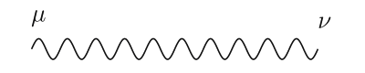
Figure 1: Photon Propagator

The two point function in TFD is a thermal doublet, and has $2\times 2$ matrix structure

$$\left(\begin{array}[]{c}A^{1}_{\mu}\\ A^{2}_{\mu}\end{array}\right)=\left(\begin{array}[]{c}A_{\mu}\\ {\tilde{A}_{\mu}^{\dagger}}\end{array}\right).$$ (46)

Then the photon propagator is

$$i\Delta^{ab}_{\mu\nu}(x-y)=\theta(t_{x}-t_{y})\langle 0(\beta)|A^{a}_{\mu}(x)A^{b}_{\nu}(y)|0(\beta)\rangle+\theta(t_{y}-t_{x})\langle 0(\beta)|A^{b}_{\nu}(y)A^{a}_{\mu}(x)|0(\beta)\rangle,$$ (47)

where $a,b=1,2$ and $\mu,\,\nu$ are tensor indices. Using the Cauchy theorem

$$\int dk^{0}\frac{e^{-ik_{0}(x_{0}-y_{0})}}{k_{0}-(\omega-i\xi)} = -2\pi ie^{-i\omega_{k}(x_{0}-y_{0})}\theta(x_{0}-y_{0}),$$

$$\int dk^{0}\frac{e^{-ik_{0}(x_{0}-y_{0})}}{k_{0}-(-\omega+i\xi)} = 2\pi ie^{i\omega_{k}(x_{0}-y_{0})}\theta(y_{0}-x_{0}),$$ (48)

then for $a=b=1$ eq. (47) becomes

$$\Delta^{11}_{\mu\nu}(x-y)=-\int\frac{d^{4}k}{(2\pi)^{4}}e^{-ik_{\rho}(x^{\rho}-y^{\rho})}\sum_{\lambda}\epsilon_{\mu}(k,\lambda)\epsilon_{\nu}(k,\lambda)\left[\frac{c_{B}^{2}(\omega)}{k_{0}^{2}-(\omega-i\xi)^{2}}-\frac{d_{B}^{2}(\omega)}{k_{0}^{2}-(\omega+i\xi)^{2}}\right].$$ (49)

Here $k_{\rho}(x^{\rho}-y^{\rho})\equiv ik_{0}(t_{x}-t_{y})-\vec{k}\cdot(\vec{x}-\vec{y})$. Calculating other components $\Delta^{12}_{\mu\nu}(x-y)$, $\Delta^{21}_{\mu\nu}(x-y)$ and $\Delta^{22}_{\mu\nu}(x-y)$, the propagator is

$$\Delta^{ab}_{\mu\nu}(x-y)=\frac{i\hbar}{(2\pi)^{4}}\int d^{4}k\,e^{ik\cdot(x-y)-ik_{0}(t_{x}-t_{y})}\Delta^{ab}_{\mu\nu}(k)$$ (50)

and

$$\Delta^{ab}_{\mu\nu}(k)=\left(\begin{array}[]{cc}\frac{c_{B}^{2}(\omega)}{k_{0}^{2}-(\omega-i\xi)^{2}}-\frac{d_{B}^{2}(\omega)}{k_{0}^{2}-(\omega+i\xi)^{2}}&\hskip 5.69046pt\frac{c_{B}(\omega)d_{B}(\omega)}{k_{0}^{2}-(\omega-i\xi)^{2}}-\frac{c_{B}(\omega)d_{B}(\omega)}{k_{0}^{2}-(\omega+i\xi)^{2}}\\ \frac{c_{B}(\omega)d_{B}(\omega)}{k_{0}^{2}-(\omega-i\xi)^{2}}-\frac{c_{B}(\omega)d_{B}(\omega)}{k_{0}^{2}-(\omega+i\xi)^{2}}&\hskip 5.69046pt\frac{d_{B}^{2}(\omega)}{k_{0}^{2}-(\omega-i\xi)^{2}}-\frac{c_{B}^{2}(\omega)}{k_{0}^{2}-(\omega+i\xi)^{2}}\end{array}\right)\eta_{\mu\nu},$$ (53)

with $\omega\equiv\omega(k)$ and $\sum_{\lambda}\epsilon_{\mu}(k,\lambda)\epsilon_{\nu}(k,\lambda)=\eta_{\mu\nu}$. In a simplified form eq. (53) is given as

$$\Delta^{ab}_{\mu\nu}(k)=U_{B}(\omega)\tau\left[k_{0}^{2}-(\omega-i\delta\tau)^{2}\right]^{-1}U_{B}(\omega)\eta_{\mu\nu},$$ (54)

where

$$U_{B}(\omega)=\left(\begin{array}[]{cc}c_{B}(\omega)&d_{B}(\omega)\\ d_{B}(\omega)&c_{B}(\omega)\end{array}\right),\quad\quad\quad\tau=\left(\begin{array}[]{cc}1&0\\ 0&-1\end{array}\right).$$ (59)

The propagator is separated as

$$\Delta_{\mu\nu}(k)=\Delta_{\mu\nu}^{(0)}(k)+\Delta_{\mu\nu}^{(\beta)}(k),$$ (60)

where $\Delta_{\mu\nu}^{(0)}(k)$ and $\Delta_{\mu\nu}^{(\beta)}(k)$ are zero and finite temperature parts respectively. Explicitly

$$\Delta_{\mu\nu}^{(0)}(k) = \frac{\eta_{\mu\nu}}{k^{2}}\tau,$$

$$\Delta_{\mu\nu}^{(\beta)}(k) = -\frac{2\pi i\delta(k^{2})}{e^{\beta k_{0}}-1}\left(\begin{array}[]{cc}1&e^{\beta k_{0}/2}\\ e^{\beta k_{0}/2}&1\end{array}\right)\eta_{\mu\nu}.$$ (63)

IV.2 The Electron Propagator

The electron propagator is given as

$$S^{ab}_{\mu\nu}(x-y)=\hbar\int\frac{d^{4}k}{(2\pi)^{4}}e^{-ik_{\rho}(x^{\rho}-y^{\rho})}S^{ab}_{\mu\nu}(k),$$ (64)

and it is represented in FIG. 2.

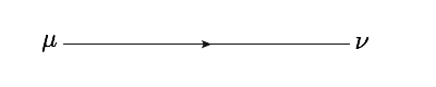
Figure 2: Fermion Propagator

This equation is written as

$$S^{ab}_{\mu\nu}(k)=\frac{1}{\hbar}\int d^{4}z\,e^{ik_{\rho}(x^{\rho}-y^{\rho})}S^{ab}_{\mu\nu}(x-y),$$ (65)

where $z=x-y$ and

$$S^{ab}_{\mu\nu}(x-y)=\theta(t_{x}-t_{y})\langle 0(\beta)|\psi^{a}_{\mu}(x)\bar{\psi}^{b}_{\nu}(y)|0(\beta)\rangle-\theta(t_{y}-t_{x})\langle 0(\beta)|\bar{\psi}^{b}_{\nu}(y)\psi^{a}_{\mu}(x)|0(\beta)\rangle,$$ (66)

with $\bar{\psi}(y)=\psi^{\dagger}(y)\gamma^{0}$ and $\mu,\nu$ being the spinors indices. Using the free Dirac field equation,

$$\psi(x)=\sum_{r}\int d^{3}k\,\left[u^{r}(k)a^{r}(k)e^{i(k\cdot x-\xi_{k}t)}+v^{r}(k)b^{r\dagger}(k)e^{-i(k\cdot x-\xi_{k}t)}\right],$$ (67)

where $a^{r}(k)$ and $b^{r}(k)$ are annihilation operators for electrons and positrons, respectively. $u^{r}(k)$ and $v^{r}(k)$ are Dirac spinors then eq. (66) becomes

$$S^{ab}_{\mu\nu}(k) = \left(\frac{\gamma^{0}\xi-\vec{\gamma}\cdot\vec{k}+m}{2\xi}\right)_{\mu\nu}\left[U_{F}(\xi)(k_{0}-\xi+i\delta\tau)^{-1}U_{F}^{\dagger}(\xi)\right]^{ab}$$ (68)

$$+ \left(\frac{\gamma^{0}\xi+\vec{\gamma}\cdot\vec{k}-m}{2\xi}\right)_{\mu\nu}\left[U_{F}(-\xi)(k_{0}+\xi+i\delta\tau)^{-1}U_{F}^{\dagger}(-\xi)\right]^{ab},$$

where Bogoliubov transformations, eq. (28), are used. Here $\xi\equiv\xi(k)$,

$$U_{F}(\xi)=\left(\begin{array}[]{cc}c_{F}(\xi)&d_{F}(\xi)\\ -d_{F}(\xi)&c_{F}(\xi)\end{array}\right),$$ (71)

and $c_{F}(\xi)$ and $d_{F}(\xi)$ are given by eq. (29).

This propagator is separated into two parts as

$$S_{\mu\nu}(k)=S_{\mu\nu}^{(0)}(k)+S_{\mu\nu}^{(\beta)}(k),$$ (72)

where

$$S_{\mu\nu}^{(0)}(k) = \frac{\not{k}+m}{k^{2}-m^{2}},$$

$$S_{\mu\nu}^{(\beta)}(k) = \frac{2\pi i}{e^{\beta k_{0}}+1}\Biggl{[}\frac{\gamma^{0}\epsilon-\vec{\gamma}\cdot\vec{k}+m}{2\epsilon}\left(\begin{array}[]{cc}1&e^{\beta k_{0}/2}\\ e^{\beta k_{0}/2}&-1\end{array}\right)\delta(k_{0}-\epsilon)$$ (75)

$$+ \frac{\gamma^{0}\epsilon+\vec{\gamma}\cdot\vec{k}-m}{2\epsilon}\left(\begin{array}[]{cc}-1&e^{\beta k_{0}/2}\\ e^{\beta k_{0}/2}&1\end{array}\right)\delta(k_{0}+\epsilon)\Biggl{]}.$$ (78)

Here $S_{\mu\nu}^{(0)}(k)$ and $S_{\mu\nu}^{(\beta)}(k)$ are zero and finite temperature parts respectively.

IV.3 The Graviton Propagator

The graviton propagator, represented in FIG. 3,

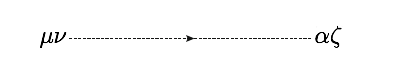
Figure 3: Graviton Propagator

is written as

$$iD^{ab}_{\mu\nu\alpha\zeta}(x-y)=\theta(t_{x}-t_{y})\langle 0(\beta)|A^{a}_{\mu\nu}(x)A^{b}_{\alpha\zeta}(y)|0(\beta)\rangle+\theta(t_{y}-t_{x})\langle 0(\beta)|A^{b}_{\alpha\zeta}(y)A^{a}_{\mu\nu}(x)|0(\beta)\rangle,$$ (79)

where $a,b=1,2$ and $\mu,\,\nu,\,\alpha,\,\zeta$ are tensor indices. The tensor $A_{\mu\nu}(x)$ is given by

$$A_{\mu\nu}(x)=\int\frac{d^{3}k}{\sqrt{2\omega_{k}(2\pi)^{3}}}\sum_{\lambda}\epsilon_{\mu\nu}(k,\lambda)\left(a_{k,\lambda}e^{-ik_{\rho}x^{\rho}}+a_{k,\lambda}^{\dagger}e^{ik_{\rho}x^{\rho}}\right),$$ (80)

with $\epsilon_{\mu\nu}(k,\lambda)$ being the polarization tensor. Using the thermal doublet,

$$\left(\begin{array}[]{c}A^{1}_{\mu\nu}\\ A^{2}_{\mu\nu}\end{array}\right)=\left(\begin{array}[]{c}A_{\mu\nu}\\ {\tilde{A}_{\mu\nu}^{\dagger}}\end{array}\right),$$ (85)

the component $a=b=1$ is given as

$$iD^{11}_{\mu\nu\alpha\zeta}(x-y) = \theta(t_{x}-t_{y})\iint\!\!\!\!\!\!\!\!\hbox{$\sum$}dp\,dk\,\epsilon_{\mu\nu}(k,\lambda)\epsilon_{\alpha\zeta}(p,\lambda^{\prime})\times$$ (86)

$$\times \langle 0(\beta)|\left(a_{k,\lambda}e^{-ik_{\rho}x^{\rho}}+a_{k,\lambda}^{\dagger}e^{ik_{\rho}x^{\rho}}\right)\left(a_{p,\lambda}e^{-ip_{\rho}y^{\rho}}+a_{p,\lambda}^{\dagger}e^{ip_{\rho}y^{\rho}}\right)|0(\beta)\rangle$$

$$+ \theta(t_{y}-t_{x})\iint\!\!\!\!\!\!\!\!\hbox{$\sum$}dp\,dk\,\epsilon_{\alpha\zeta}(p,\lambda^{\prime})\epsilon_{\mu\nu}(k,\lambda)\times$$

$$\times \langle 0(\beta)|\left(a_{p,\lambda}e^{-ip_{\rho}y^{\rho}}+a_{p,\lambda}^{\dagger}e^{ip_{\rho}y^{\rho}}\right)\left(a_{k,\lambda}e^{-ik_{\rho}x^{\rho}}+a_{k,\lambda}^{\dagger}e^{ik_{\rho}x^{\rho}}\right)|0(\beta)\rangle,$$

where $\iint\!\!\!\!\!\!\!\!\hbox{$\sum$}dp\,dk\equiv\int\frac{d^{3}k}{\sqrt{2\omega_{k}(2\pi)^{3}}}\int\frac{d^{3}p}{\sqrt{2\omega_{p}(2\pi)^{3}}}\sum_{\lambda,\lambda^{\prime}}$ has been used. Using Bogoliubov transformations, eq. (25), and commutation relations, eq. (27), the propagator is

$$iD^{11}_{\mu\nu\alpha\zeta}(x-y) = -\theta(t_{x}-t_{y})\iint\!\!\!\!\!\!\!\!\hbox{$\sum$}dp\,dk\,\epsilon_{\mu\nu}(k,\lambda)\epsilon_{\alpha\zeta}(p,\lambda^{\prime})\times$$ (87)

$$\times \left[c_{B}^{2}(\omega)\delta^{3}(k-p)e^{-ik_{\rho}x^{\rho}+ip_{\rho}y^{\rho}}+d_{B}^{2}(\omega)\delta^{3}(k-p)e^{ik_{\rho}x^{\rho}-ip_{\rho}y^{\rho}}\right]$$

$$- \theta(t_{y}-t_{x})\iint\!\!\!\!\!\!\!\!\hbox{$\sum$}dp\,dk\,\epsilon_{\alpha\zeta}(p,\lambda^{\prime})\times$$

$$\times \left[c_{B}^{2}(\omega)\delta^{3}(p-k)e^{-ip_{\rho}y^{\rho}+ik_{\rho}x^{\rho}}+d_{B}^{2}(\omega)\delta^{3}(p-k)e^{ip_{\rho}y^{\rho}-ik_{\rho}x^{\rho}}\right].$$

Applying the Cauchy theorem, eq. (48), we get

$$D^{11}_{\mu\nu\alpha\zeta}(x-y)=-\int\frac{d^{4}k}{(2\pi)^{4}}e^{-ik_{\rho}(x^{\rho}-y^{\rho})}\left[\frac{c_{B}^{2}(\omega)}{k_{0}^{2}-(\omega-i\xi)^{2}}-\frac{d_{B}^{2}(\omega)}{k_{0}^{2}-(\omega+i\xi)^{2}}\right]\varepsilon_{\mu\nu\alpha\zeta},$$ (88)

with

$$\sum_{\lambda}\epsilon_{\mu\nu}(k,\lambda)\epsilon_{\alpha\zeta}(k,\lambda)=\frac{1}{2}\left(\eta_{\mu\alpha}\eta_{\nu\zeta}+\eta_{\mu\zeta}\eta_{\nu\alpha}-\eta_{\mu\nu}\eta_{\alpha\zeta}\right)\equiv\varepsilon_{\mu\nu\alpha\zeta}.$$ (89)

The component with $a=1,\,b=2$ is written as

$$iD^{12}_{\mu\nu\alpha\zeta}(x-y)=\theta(t_{x}-t_{y})\langle 0(\beta)|A_{\mu\nu}(x)\tilde{A}_{\alpha\zeta}^{\dagger}(y)|0(\beta)\rangle+\theta(t_{y}-t_{x})\langle 0(\beta)|\tilde{A}_{\alpha\zeta}^{\dagger}(y)A_{\mu\nu}(x)|0(\beta)\rangle,$$ (90)

where the doublet notation is used. This component is written as

$$D^{12}_{\mu\nu\alpha\zeta}(x-y)=-\int\frac{d^{4}k}{(2\pi)^{4}}e^{-ik_{\rho}(x^{\rho}-y^{\rho})}\left[\frac{c_{B}(\omega)d_{B}(\omega)}{k_{0}^{2}-(\omega-i\xi)^{2}}-\frac{c_{B}(\omega)d_{B}(\omega)}{k_{0}^{2}-(\omega+i\xi)^{2}}\right]\varepsilon_{\mu\nu\alpha\zeta}.$$ (91)

In addition we have

$$D^{21}_{\mu\nu\alpha\zeta}(x-y)=D^{12}_{\mu\nu\alpha\zeta}(x-y).$$ (92)

For the component $a=b=2$, we get

$$iD^{22}_{\mu\nu\alpha\zeta}(x-y) = \theta(t_{x}-t_{y})\langle 0(\beta)|\tilde{A}_{\mu\nu}^{\dagger}(x)\tilde{A}_{\alpha\zeta}^{\dagger}(y)|0(\beta)\rangle+\theta(t_{y}-t_{x})\langle 0(\beta)|\tilde{A}_{\alpha\zeta}^{\dagger}(y)\tilde{A}_{\mu\nu}^{\dagger}(x)|0(\beta)\rangle,$$ (93)

$$= -\int\frac{d^{4}k}{(2\pi)^{4}}e^{-ik_{\rho}(x^{\rho}-y^{\rho})}\left[\frac{d_{B}^{2}(\omega)}{k_{0}^{2}-(\omega-i\xi)^{2}}-\frac{c_{B}^{2}(\omega)}{k_{0}^{2}-(\omega+i\xi)^{2}}\right]\varepsilon_{\mu\nu\alpha\zeta}.$$

Combining eqs. (88), (91), (92) and (93) the graviton propagator is

$$D^{ab}_{\mu\nu\alpha\zeta}(x-y)=-\int\frac{d^{4}k}{(2\pi)^{4}}e^{-ik_{\rho}(x^{\rho}-y^{\rho})}\,D^{ab}_{\mu\nu\alpha\zeta}(k),$$ (94)

where

$$D^{ab}_{\mu\nu\alpha\zeta}(k)=\left(\begin{array}[]{cc}\frac{c_{B}^{2}(\omega)}{k_{0}^{2}-(\omega-i\xi)^{2}}-\frac{d_{B}^{2}(\omega)}{k_{0}^{2}-(\omega+i\xi)^{2}}&\hskip 5.69046pt\frac{c_{B}(\omega)d_{B}(\omega)}{k_{0}^{2}-(\omega-i\xi)^{2}}-\frac{c_{B}(\omega)d_{B}(\omega)}{k_{0}^{2}-(\omega+i\xi)^{2}}\\ \frac{c_{B}(\omega)d_{B}(\omega)}{k_{0}^{2}-(\omega-i\xi)^{2}}-\frac{c_{B}(\omega)d_{B}(\omega)}{k_{0}^{2}-(\omega+i\xi)^{2}}&\hskip 5.69046pt\frac{d_{B}^{2}(\omega)}{k_{0}^{2}-(\omega-i\xi)^{2}}-\frac{c_{B}^{2}(\omega)}{k_{0}^{2}-(\omega+i\xi)^{2}}\end{array}\right)\,\varepsilon_{\mu\nu\alpha\zeta}.$$ (97)

Then eq. (97) is written in the following form:

$$D^{ab}_{\mu\nu\alpha\zeta}(k)=U_{B}(\omega)\tau\left[k_{0}^{2}-(\omega-i\delta\tau)^{2}\right]^{-1}U_{B}(\omega)\varepsilon_{\mu\nu\alpha\zeta},$$ (98)

where $U_{B}(\omega)$ and $\tau$ are given in eq. (59).

The graviton propagator is written as

$$D_{\mu\nu\alpha\zeta}(k)=D_{\mu\nu\alpha\zeta}^{(0)}(k)+D_{\mu\nu\alpha\zeta}^{(\beta)}(k),$$ (99)

with

$$D_{\mu\nu\alpha\zeta}^{(0)}(k) = \frac{\eta_{\mu\alpha}\eta_{\nu\zeta}+\eta_{\mu\zeta}\eta_{\nu\alpha}-\eta_{\mu\nu}\eta_{\alpha\zeta}}{2k^{2}}\,\tau,$$

$$D_{\mu\nu\alpha\zeta}^{(\beta)}(k) = -\frac{\pi i\delta(k^{2})}{e^{\beta k_{0}}-1}\left(\begin{array}[]{cc}1&e^{\beta k_{0}/2}\\ e^{\beta k_{0}/2}&1\end{array}\right)(\eta_{\mu\alpha}\eta_{\nu\zeta}+\eta_{\mu\zeta}\eta_{\nu\alpha}-\eta_{\mu\nu}\eta_{\alpha\zeta}),$$ (102)

where $D_{\mu\nu\alpha\zeta}^{(0)}(k)$ and $D_{\mu\nu\alpha\zeta}^{(\beta)}(k)$ are zero and finite temperature parts respectively.

V Gravitation interacting with photons and fermions at finite temperature

Transition amplitudes, ${\cal M}$, of various scattering processes involving gravitons, photons and fermions at finite temperature are calculated. The vertex factors are:

1. Graviton-Photon vertex factor

   

2. Fermion-Photon vertex factor

   

3. Graviton-Fermion vertex factor

   

4. Graviton-Fermion-Photon vertex factor

   

V.1 Gravitational M$\varnothing$ller scattering

The diagrams are similar to the traditional M$\varnothing$ller scattering, where the photon is replaced by a graviton. The two diagrams that describe this scattering are given in FIG. 4.

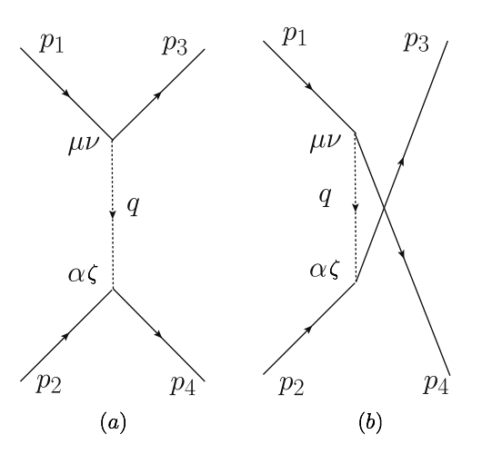
Figure 4: Feynman diagram for M$\varnothing$ller scattering

The total transition amplitude is given by

$${\cal M}={\cal M}_{1}+{\cal M}_{2},$$ (103)

where ${\cal M}_{1}$ and ${\cal M}_{2}$ are scattering amplitudes for processes given in FIG. 4 (a) and (b) respectively. These contributions are

$${\cal M}_{1} = {\cal M}_{01}+{\cal M}_{\beta 1},$$ (104)

$${\cal M}_{2} = {\cal M}_{02}+{\cal M}_{\beta 2},$$ (105)

where ${\cal M}_{0i}$ and ${\cal M}_{\beta i}$ are zero and finite temperature parts of the amplitude respectively. Thus

$${\cal M}_{1}=\bar{u}_{3}\left[-\frac{i\hbar c\kappa}{4}(\gamma^{\mu}p_{1}^{\nu}+p_{3}^{\mu}\gamma^{\nu})\right]{u}_{1}\,D_{\mu\nu\alpha\zeta}(q)\,\bar{u}_{4}\left[-\frac{i\hbar c\kappa}{4}(\gamma^{\alpha}p_{2}^{\zeta}+p_{4}^{\alpha}\gamma^{\zeta})\right]{u}_{2},$$ (106)

where $D_{\mu\nu\alpha\zeta}(q)$ is the graviton propagator given in eq. (99). Zero temperature transition amplitude is

$${\cal M}_{01}=-\frac{\hbar^{2}c^{2}\kappa^{2}}{32(p_{1}-p_{3})^{2}}\left[\bar{u}_{3}(\gamma^{\mu}p_{1}^{\nu}+p_{3}^{\mu}\gamma^{\nu})u_{1}\right]\tau\{\bar{u}_{4}[\gamma_{\mu}(p_{2}+p_{4})_{\nu}+\gamma_{\nu}(p_{2}+p_{4})_{\mu}-\eta_{\mu\nu}(\not{p}_{2}+\not{p}_{4})]u_{2}\},$$ (107)

and finite temperature transition amplitude is

$${\cal M}_{\beta 1} = \frac{\hbar^{2}c^{2}\kappa^{2}}{16}\left[\bar{u}_{3}(\gamma^{\mu}p_{1}^{\nu}+p_{3}^{\mu}\gamma^{\nu})u_{1}\right]\frac{i\pi\delta(q^{2})}{e^{\beta q_{0}}-1}\left(\begin{array}[]{cc}1&e^{\beta q_{0}/2}\\ e^{\beta q_{0}/2}&1\end{array}\right)\times$$ (110)

$$\times \{\bar{u}_{4}[\gamma_{\mu}(p_{2}+p_{4})_{\nu}+\gamma_{\nu}(p_{2}+p_{4})_{\mu}-\eta_{\mu\nu}(\not{p}_{2}+\not{p}_{4})]u_{2}\}.$$ (111)

Then eq. (104) is written as

$${\cal M}_{1} = -\frac{\hbar^{2}c^{2}\kappa^{2}}{16}\left[\bar{u}_{3}(\gamma^{\mu}p_{1}^{\nu}+p_{3}^{\mu}\gamma^{\nu})u_{1}\right]\{\bar{u}_{4}[\gamma_{\mu}(p_{2}+p_{4})_{\nu}+\gamma_{\nu}(p_{2}+p_{4})_{\mu}-\eta_{\mu\nu}(\not{p}_{2}+\not{p}_{4})]u_{2}\}\times$$ (114)

$$\times \left[\frac{\tau}{2(p_{1}-p_{3})^{2}}-\frac{i\pi\delta(q^{2})}{e^{\beta q_{0}}-1}\left(\begin{array}[]{cc}1&e^{\beta q_{0}/2}\\ e^{\beta q_{0}/2}&1\end{array}\right)\right].$$

And eq. (105) is

$${\cal M}_{2} = -\frac{\hbar^{2}c^{2}\kappa^{2}}{16}\left[\bar{u}_{4}(\gamma^{\mu}p_{1}^{\nu}+p_{4}^{\mu}\gamma^{\nu})u_{1}\right]\{\bar{u}_{3}[\gamma_{\mu}(p_{2}+p_{3})_{\nu}+\gamma_{\nu}(p_{2}+p_{3})_{\mu}-\eta_{\mu\nu}(\not{p}_{2}+\not{p}_{3})]u_{2}\}\times$$ (117)

$$\times \left[\frac{\tau}{2(p_{1}-p_{4})^{2}}-\frac{i\pi\delta(q^{2})}{e^{\beta q_{0}}-1}\left(\begin{array}[]{cc}1&e^{\beta q_{0}/2}\\ e^{\beta q_{0}/2}&1\end{array}\right)\right].$$

V.2 Gravitational Compton scattering

The gravitational Compton scattering is analyzed and following diagrams are considered.

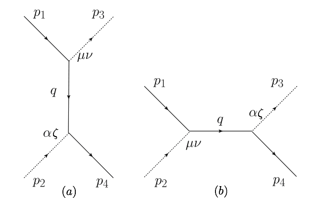
Figure 5: Feynman diagram for Compton scattering

The transition amplitude of the gravitational Compton scattering is

$${\cal M}={\cal M}_{1}+{\cal M}_{2},$$ (118)

where ${\cal M}_{1}$ and ${\cal M}_{2}$ are scattering amplitudes for processes given in FIG. 5 (a) and (b) respectively.

$${\cal M}_{1} = \bar{u}_{4}\xi^{*}_{3\mu\nu}\left[-\frac{i\hbar c\kappa}{4}(\gamma^{\mu}p_{1}^{\nu}+(p_{1}-p_{3})^{\mu}\gamma^{\nu})\right]\,S(q)\,\left[-\frac{i\hbar c\kappa}{4}(\gamma^{\alpha}(p_{4}-p_{2})^{\zeta}+p_{4}^{\alpha}\gamma^{\zeta})\right]u_{1}\xi_{2\alpha\zeta},$$ (119)

$${\cal M}_{2} = \bar{u}_{4}\xi^{*}_{3\mu\nu}\left[-\frac{i\hbar c\kappa}{4}(\gamma^{\mu}p_{1}^{\nu}+(p_{1}+p_{2})^{\mu}\gamma^{\nu})\right]\,S(q)\,\left[-\frac{i\hbar c\kappa}{4}(\gamma^{\alpha}(p_{3}+p_{4})^{\zeta}+p_{4}^{\alpha}\gamma^{\zeta})\right]u_{1}\xi_{2\alpha\zeta},$$ (120)

where $S(q)$ is the fermion propagator given in eq. (72). Thus transition amplitude are

$${\cal M}_{1} = -\frac{\hbar^{2}c^{2}\kappa^{2}}{16}\left[\bar{u}_{4}(2\vec{p}_{4}-\vec{p}_{2})\cdot\vec{\xi}_{2}\not{\xi}_{2}\right]\left[\not{\xi}_{3}^{*}\vec{\xi}_{3}^{*}\cdot(2\vec{p}_{1}-\vec{p}_{3})u_{1}\right]\left[\frac{(\not{p}_{1}-\not{p}_{3}+m)}{(p_{1}-p_{3})^{2}-m^{2}}-{\cal F}(\beta)\right],$$ (121)

and

$${\cal M}_{2} = -\frac{\hbar^{2}c^{2}\kappa^{2}}{16}\left[\bar{u}_{4}(2\vec{p}_{4}+\vec{p}_{3})\cdot\vec{\xi}_{3}^{*}\not{\xi}_{3}^{*}\right]\left[\not{\xi}_{2}\vec{\xi}_{2}\cdot(2\vec{p}_{1}+\vec{p}_{2})u_{1}\right]\left[\frac{(\not{p}_{1}+\not{p}_{2}+m)}{(p_{1}+p_{2})^{2}-m^{2}}-{\cal F}(\beta)\right],$$ (122)

where

$${\cal F}(\beta) \equiv \frac{2\pi i}{e^{\beta q_{0}}+1}\Biggl{[}\frac{\gamma^{0}\epsilon-\vec{\gamma}\cdot\vec{q}+m}{2\epsilon}\left(\begin{array}[]{cc}1&e^{\beta q_{0}/2}\\ e^{\beta q_{0}/2}&-1\end{array}\right)\delta(q_{0}-\epsilon)$$ (125)

$$+ \frac{\gamma^{0}\epsilon+\vec{\gamma}\cdot\vec{q}+m}{2\epsilon}\left(\begin{array}[]{cc}-1&e^{\beta q_{0}/2}\\ e^{\beta q_{0}/2}&1\end{array}\right)\delta(q_{0}+\epsilon)\Biggl{]}.$$ (128)

The graviton polarization tensor $\epsilon_{\mu\nu}$ is taken as the product of two spin-1 polarization vectors $\epsilon_{\mu}$ and $\epsilon_{\nu}$, i.e., $\epsilon_{\mu\nu}=\epsilon_{\mu}\epsilon_{\nu}$.

V.3 Graviton photoproduction amplitudes

The photoproduction of gravitons, such as Born and four-point interaction diagrams, are considered.

V.3.1 Born diagram

The Feynman diagram that describes this process is given as follows.

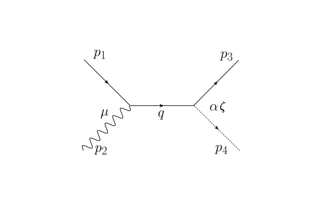
Figure 6: Graviton photoproduction: Born diagram

The transition amplitude is written as

$${\cal M}=\bar{u}_{3}\,\xi^{*}_{4\alpha\zeta}\left[ie\gamma^{\mu}\right]\xi_{2\mu}\,S(q)\,\left[-\frac{i\hbar c\kappa}{4}(\gamma^{\alpha}(p_{1}+p_{2})^{\zeta}+p_{3}^{\alpha}\gamma^{\zeta})\right]u_{1}.$$ (129)

Using the fermion propagator $S(q)$ given in eq. (72) we get

$${\cal M}=\frac{e\hbar c\kappa}{4}\left[\bar{u}_{3}(\vec{p}_{1}+\vec{p}_{2}+\vec{p}_{3})\cdot\vec{\xi}^{*}_{4}\not{\xi}_{4}\right]\left[\not{\xi}_{2}u_{1}\right]\left[\frac{(\not{p}_{1}+\not{p}_{2}+m)}{(p_{1}+p_{2})^{2}-m^{2}}+{\cal F}(\beta)\right],$$ (130)

where ${\cal F}(\beta)$ is given in eq. (128).

V.3.2 Four-point interaction diagram

The second process which describes graviton photoproduction is represented by

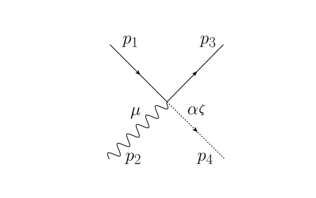
Figure 7: Graviton photoproduction: four-point interaction

The transition amplitude for this scattering is

$${\cal M} = \bar{u}_{3}\,\xi^{*}_{4\alpha\zeta}\left[\frac{ie\kappa}{2}\gamma^{\zeta}\eta^{\alpha\mu}\right]\xi_{2\mu}u_{1}$$ (131)

$$= \frac{ie\kappa}{2}\left[\bar{u}_{3}\not{\xi}^{*}_{4}\vec{\xi}^{*}_{4}\cdot\vec{\xi}_{2}u_{1}\right].$$

In this process, there is no temperature contribution, i.e., the temperature does not affect this interaction.

VI Conclusions

The theory of gravitoelectromagnetism arises from comparisons between the Newtonian gravity and the Coulomb law. A possible theory for GEM, a gravity theory similar to electromagnetic theory, emerges when the Weyl tensor is considered. The Weyl tensor is divided into two parts, gravitoelectric and gravitomagnetic fields, and the field equations are similar to Maxwell equations. A gravitoelectromagnetic tensor potential leads to a lagrangian formalism. The graviton field is described analogous to electromagnetism and thus provides us with an alternative way to study the interaction of the graviton with fermions and photons in flat space-time. It leads to a perturbation series and transition amplitudes for various scattering processes are considered. GEM at finite temperature using TFD formalism is established.

The graviton, fermion and photon propagators in the TFD formalism are written in two parts, one at T=0 and the other at finite temperature. Transition amplitudes for the gravitational M$\varnothing$ller and Compton scattering and graviton photoproduction at finite temperature are calculated. The transition amplitudes are consist of two parts. These results will have implications for astrophysical processes.

References

- (1) J. C. Maxwell, Phil. Trans. Soc. Lond. 155, 492 (1865).
- (2) O. Heaviside, Electrician 31, 259 (1893).
- (3) O. Heaviside, Electrician 31, 281 (1893).
- (4) H. Thirring, Physikalische Zeitschrift 19, 204 (1918).
- (5) A. Matte, Can. J. Math 5, 1 (1953).
- (6) W. B. Campbell and T. A. Morgan, Physica 53, 264 (1971).
- (7) W. B. Campbell, Gen. Relativ. Gravit. 4, 137 (1973).
- (8) W. B. Campbell and T. A. Morgan, Am. J. Phys. 44, 356 (1976).
- (9) W. B. Campbell, J. Macek and T. A. Morgan, Phys. Rev. D 15, 2156 (1977).
- (10) V. B. Braginsky, C. M. Caves and K. S. Thorne, Phys. Rev. D 15, 2047 (1977).
- (11) J. Ramos and R. Gilmore, Int. J. Mod. Phys. D 15, 505 (2006).
- (12) J. Ramos, Gen. Relativ. Gravit. 38, 773 (2006).
- (13) J. Lense and H. Thirring, Physikalische Zeitschrift 19, 156 (1918).
- (14) I. Ciufolini and J. A. Wheeler, Gravitation and Inertia, Princeton University Press, Princeton, (1951).
- (15) K. Nordtvedt, Rev. Phys. Lett. 61, 2647 (1988).
- (16) M. Soffel, S. Klioner, J. Muller and L. Biskupek, Phys. Rev. D 78, 024033 (2008).
- (17) C. W. F. Everitt et al., Phys. Rev. Lett. 106, 221101 (2011).
- (18) B. Mashhoon Gravitoelectromagnetism: A Brief Review, [arXiv:gr-qc/0311030].
- (19) L. Filipe Costa and Carlos A. R. Herdeiro, Phys. Rev. D 78, 024021 (2008).
- (20) R. Maartens and B. A. Bassett, Class. Quant. Grav. 15, 705 (1998).
- (21) J. Ramos, M. de Montigny and F. C. Khanna, Gen. Rel. Grav. 42, 2403 (2010).
- (22) Y. Takahashi and H. Umezawa, Coll. Phenomena 2, 55 (1975); Int. Jour. Mod. Phys. B 10, 1755 (1996).
- (23) Y. Takahashi, H. Umezawa and H. Matsumoto, Thermofield Dynamics and Condensed States, North-Holland, Amsterdan, (1982); F. C. Khanna, A. P. C. Malbouisson, J. M. C. Malboiusson and A. E. Santana, Themal quantum field theory: Algebraic aspects and applications, World Scientific, Singapore, (2009).
- (24) H. Umezawa, Advanced Field Theory: Micro, Macro and Thermal Physics, AIP, New York, (1993).
- (25) A. E. Santana and F. C. Khanna, Phys. Lett. A 203, 68 (1995).
- (26) A. E. Santana, F. C. Khanna, H. Chu, and C. Chang, Ann. Phys. 249, 481 (1996).