Fairness in Learning: Classic and Contextual Bandits

Abstract

We introduce the study of fairness in multi-armed bandit problems. Our fairness definition can be interpreted as demanding that given a pool of applicants (say, for college admission or mortgages), a worse applicant is never favored over a better one, despite a learning algorithm’s uncertainty over the true payoffs. We prove results of two types:

First, in the important special case of the classic stochastic bandits problem (i.e. in which there are no contexts), we provide a provably fair algorithm based on “chained” confidence intervals, and prove a cumulative regret bound with a cubic dependence on the number of arms. We further show that any fair algorithm must have such a dependence. When combined with regret bounds for standard non-fair algorithms such as UCB, this proves a strong separation between fair and unfair learning, which extends to the general contextual case.

In the general contextual case, we prove a tight connection between fairness and the KWIK (Knows What It Knows) learning model: a KWIK algorithm for a class of functions can be transformed into a provably fair contextual bandit algorithm, and conversely any fair contextual bandit algorithm can be transformed into a KWIK learning algorithm. This tight connection allows us to provide a provably fair algorithm for the linear contextual bandit problem with a polynomial dependence on the dimension, and to show (for a different class of functions) a worst-case exponential gap in regret between fair and non-fair learning algorithms.

1 Introduction

Automated techniques from statistics and machine learning are increasingly being used to make decisions that have important consequences on people’s lives, including hiring (Miller, 2015), lending (Byrnes, 2016), policing (Rudin, 2013), and even criminal sentencing (Barry-Jester et al., 2015). These high stakes uses of machine learning have led to increasing concern in law and policy circles about the potential for (often opaque) machine learning techniques to be discriminatory or unfair (Coglianese and Lehr, 2016; Barocas and Selbst, 2016). Moreover, these concerns are not merely hypothetical: Sweeney (2013) observed that contextual ads for public record services shown in response to Google searches for stereotypically African American names were more likely to contain text referring to arrest records, compared to comparable ads shown in response to searches for stereotypically Caucasian names, which showed more neutral text. She confirmed that this was not because of stated preferences of the advertisers, but rather the automated outcome of Google’s targeting algorithms. Despite the recognized importance of this problem, very little is known about technical solutions to the problem of “unfairness”, or the extent to which “fairness” is in conflict with the goals of learning.

In this paper, we consider the extent to which a natural fairness notion is compatible with learning in a general setting (the contextual bandit setting), which can be used to model many of the applications mentioned above in which machine learning is currently employed. In this model, the learner is a sequential decision maker, which must choose at each time step $t$ which decision to make, out of a finite set of $k$ choices (for example, which of $k$ loan applicants – potentially from different populations or racial groups – to give a loan to). Before the learner makes its decision at round $t$, it observes some context $x_{j}^{t}$ for each choice of arm $j$ ($x_{j}^{t}$ could, for example, represent the contents of the loan application of an individual from population $j$ at round $t$). When the learner chooses arm $j$ at time $t$, it obtains a stochastic reward $r_{j}^{t}$ whose expectation is determined by some unknown function of the context: $\mathbb{E}\left[r_{j}^{t}\right]=f_{j}(x_{j}^{t})$. The goal of the learning algorithm is to maximize its expected reward – i.e. to approximate the optimal policy, which at each round, chooses arm $j$ to maximize $\mathbb{E}\left[r_{j}^{t}\right]$. The difficulty in this task stems from the unknown functions $f_{j}$ which map contexts to rewards; these functions must be learned. Despite this, there are many known algorithms for learning the optimal policy (in the absence of any fairness constraint).

1.1 Fairness and Learning

Our notion of individual fairness is very simple: it states that it is unfair to preferentially choose one individual (e.g. for a loan, a job, admission to college, etc.) over another if he or she is not as qualified as the other individual. This definition of fairness is apt for our setting, since in contextual learning, the quality of an arm is clear: its expected reward. We view different arms $j$ as representing different populations (e.g. different ethnic groups, cultures, or other divisions within society), and view the context $x_{j}^{t}$ at round $t$ as representing information about a particular individual from that population. Each population has its own underlying function $f_{j}$ which maps contexts to expected payoff. At each time step $t$, the algorithm is asked to choose between specific members of each population, represented by the contexts $x_{j}^{t}$. The quality of an individual is thus exactly $\mathbb{E}\left[r_{j}^{t}\right]=f_{j}(x_{j}^{t})$. Our fairness condition translates thus: for any pair of arms $j,j^{\prime}$ at time $t$, if $f_{j}(x_{j}^{t})\geq f_{j^{\prime}}(x_{j^{\prime}}^{t})$, then an algorithm is said to be discriminatory if it preferentially chooses the lower quality arm $j^{\prime}$. Said another way, an algorithm is fair if it guarantees the following: with high probability, over all rounds $t$, and for all pairs of arms $j,j^{\prime}$, whenever $f_{j}(x_{j}^{t})\geq f_{j^{\prime}}(x_{j^{\prime}}^{t})$, the algorithm chooses arm $j$ with probability at least that with which it chooses arm $j^{\prime}$.

It is worth noting that this definition of fairness (formalized in the preliminaries) is entirely consistent with the optimal policy, which can simply choose at each round to play uniformly at random from the arms $\operatorname*{arg\,max}_{j}\left(\mathbb{E}\left[r_{j}^{t}\right]\right)$ which maximize the expected reward. This is because – it seems – the goal of fairness as enunciated above is entirely consistent with the goal of maximizing expected reward. Indeed, the fairness constraint exactly states that the algorithm cannot favor low reward arms!

Our main conceptual result is that this intuition is incorrect in the face of unknown reward functions. Even though the constraint of fairness is consistent with implementing the optimal policy, it is not necessarily consistent with learning the optimal policy. We show that fairness always has a cost, in terms of the achievable learning rate of the algorithm. For some problems, the cost is mild, but for others, the cost is large.

1.2 Our Results

We divide our results into two parts. First, we study the classic stochastic multi-armed bandit problem (Lai and Robbins, 1985; Katehakis and Robbins, 1995). In this case, there are no contexts, and each arm $i$ has a fixed but unknown average reward $\mu_{i}$. Note that this is a special case of the contextual bandit problem in which the contexts are the same every day. In this setting, our fairness constraint specializes to require that with probability $1-\delta$, for any pair of arms $i,j$ for which $\mu_{i}\geq\mu_{j}$, at no round $t$ does the algorithm play arm $j$ with probability higher than that with which it plays arm $i$. Note that even this special case models interesting scenarios from the point of view of fairness in learning. It models, for example, the case in which choices are made by a loan officer after applicants have been categorized into $k$ internally indistinguishable equivalence classes based on their applications.

Without a fairness constraint, it is known that it is possible to guarantee non-trivial regret to the optimal policy after only $T=O(k)$ many rounds (Auer et al., 2002). In Section 3, we give an algorithm that satisfies our fairness constraint and is able to guarantee non-trivial regret after $T=O(k^{3})$ rounds. We then show in Section 4 that it is not possible to do better – any fair learning algorithm can be forced to endure constant per-round regret for $T=\Omega(k^{3})$ rounds. Thus, we tightly characterize the optimal regret attainable by fair algorithms in this setting, and formally separate it from the regret attainable by algorithms absent a fairness constraint. Note that this already shows a separation between the best possible learning rates for contextual bandit learning with and without the fairness constraint – the stochastic multi-armed bandit problem is a special case of every contextual bandit problem, and for general contextual bandit problems, it is also known how to get non-trivial regret after only $T=O(k)$ many rounds  (Agarwal et al., 2014; Beygelzimer et al., 2011; Chu et al., 2011).

We then move on to the general contextual bandit setting and prove a broad characterization result, relating fair contextual bandit learning to KWIK learning (Li et al., 2011). The KWIK model, which stands for Knows What it Knows and has a close relationship with reinforcement learning, is a model of sequential supervised classification in which the learning algorithm must be confident in its predictions. Informally, a KWIK learning algorithm receives a sequence of unlabeled examples, whose true labels are defined by some unknown function in a class $C$. For each example, the algorithm may either predict a label, or announce “I Don’t Know”. The KWIK requirement is that with high probability, for each example, if the algorithm predicts a label, then its prediction must be very close to the true label. The quality of a KWIK learning algorithm is characterized by its “KWIK bound”, which provides an upper bound on the maximum number of times the algorithm can be forced to announce “I Don’t Know”. For any contextual bandit problem (defined by the set of functions $C$ from which the payoff functions $f_{j}$ may be selected), we show that the optimal learning rate of any fair algorithm is determined by the best KWIK bound for the class $C$. We prove this constructively – we give a reduction showing how to convert a KWIK learning algorithm into a fair contextual bandit algorithm in Section 5, and vice versa in Section 6. Both reductions show that the KWIK bound of the KWIK algorithm is polynomially related to the regret of the fair algorithm.

This general connection has immediate implications, because it allows us to import known results for KWIK learning (Li et al., 2011). For example, it implies that some fair contextual bandit problems are easy, in that there are fair algorithms which can obtain non-trivial regret guarantees after polynomially many rounds. This is the case, for example, for the important linear special case in which the contexts $x_{j}^{t}\in\mathbb{R}^{d}$ are real valued vectors and the unknown functions $f_{j}$ are linear: $f_{j}(x_{j}^{t})=\langle\theta^{j},x_{j}^{t}\rangle$. In this case, the KWIK-learnability of noisy linear regression problems (Strehl and Littman, 2008; Li et al., 2011) implies that we can construct a fair contextual bandit algorithm whose per-round regret is polynomial in $d$. Conversely, it also implies that some contextual bandit problems which are easy without the fairness constraint become hard once we impose the fairness constraint, in that any fair algorithm must suffer constant per-round regret for exponentially many rounds. This is the case, for example, when the context consists of boolean vectors $x_{j}^{t}\in\{0,1\}^{d}$, and the unknown functions $f_{j}:\{0,1\}^{d}\rightarrow\{0,1\}$ are conjunctions – the “and”s of some unknown set of features. The impossibility of non-trivial KWIK-learning of conjunctions (Li, 2009; Li et al., 2011) implies that no fair learner in the contextual bandit setting can achieve non-trivial regret before exponentially many (in $d$) rounds.

1.3 Other Related Work

Several papers study the problem of fairness in machine learning. One line of work aims to give algorithms for batch classification which achieve group fairness otherwise known as equality of outcomes, statistical parity – or algorithms that avoid disparate impact (see e.g. Calders and Verwer (2010); Luong et al. (2011); Kamishima et al. (2011); Feldman et al. (2015); Fish et al. (2016) and Adler et al. (2016) for a study of auditing existing algorithms for disparate impact). While statistical parity is sometimes a desirable goal – indeed, it is sometimes required by law – as observed by Dwork et al. (2012) and others, it suffers from two problems. First, if different populations indeed have different statistical properties, then it can be at odds with accurate classification. Second, even in cases when statistical parity is attainable with an optimal classifier, it does not prevent discrimination at an individual level – see Dwork et al. (2012) for a catalog of ways in which statistical parity can be insufficient from the perspective of fairness. In contrast, we study a notion aimed at guaranteeing fairness at the individual level.

Our definition of fairness is most closely related to that of Dwork et al. (2012), who proposed and explored the basic properties of a technical definition of individual fairness formalizing the idea that “similar individuals should be treated similarly”. Specifically, their work presupposes the existence of a task-specific metric on individuals, and proposes that fair algorithms should satisfy a Lipschitz condition with respect to this metric. Our definition of fairness is similar, in that the expected reward of each arm is a natural metric through which we define fairness. The main conceptual distinction between our work and Dwork et al. (2012) is that their work operates under the assumption that the metric is known to the algorithm designer, and hence in their setting, the fairness constraint binds only insofar as it is in conflict with the desired outcome of the algorithm designer. The most challenging aspect of this approach (as they acknowledge) is that it requires that some third party design a “fair” metric on individuals, which in a sense encodes much of the relevant challenge. The question of how to design such a metric was considered by Zemel et al. (2013), who study methods to learn representations that encode the data, while obscuring protected attributes. Our fairness constraint, conversely, is entirely aligned with the goal of the algorithm designer in that it is satisfied by the optimal policy; nevertheless, it affects the space of feasible learning algorithms, because it interferes with learning an optimal policy, which depends on the unknown reward functions.

At a technical level, our work is related to Amin et al. (2012) and Amin et al. (2013), which also relate KWIK learning to bandit learning in a different context, unrelated to fairness (when the arm space is very large).

2 Preliminaries

We study the contextual bandit setting, which is defined by a domain $\mathcal{X}$, a set of “arms” $[k]:=\{1,\ldots,k\}$ and a class $C$ of functions of the form $f:\mathcal{X}\rightarrow[0,1]$. For each arm $j$ there is some function $f_{j}\in C$, unknown to the learner. In rounds $t=1,\ldots,T$, an adversary reveals to the algorithm a context $x_{j}^{t}$ for each arm. An algorithm $\mathcal{A}$ then chooses an arm $i_{t}$, and observes stochastic reward $r^{t}_{i_{t}}$ for the arm it chose. We assume $r^{t}_{j}\sim\mathcal{D}^{t}_{j}$, $\mathbb{E}\left[r^{t}_{j}\right]=f_{j}(x^{t}_{j})$, for some distribution $\mathcal{D}^{t}_{j}$ over $[0,1]$.

Let $\Pi$ be the set of policies mapping contexts to distributions over arms $X^{k}\to\Delta^{k}$, and $\pi^{*}$ the optimal policy which selects a distribution over arms as a function of contexts to maximize the expected reward of those arms. The pseudo-regret of an algorithm $\mathcal{A}$ on contexts $x^{1},\ldots,x^{T}$ is defined as follows, where $\pi^{t}$ represents $\mathcal{A}$’s distribution on arms at round $t$:

$$\sum_{t}\mathbb{E}_{i^{t}_{*}\sim\pi^{*}(x^{t})}\left[f_{i^{t}_{*}}(x^{t}_{i^{t}_{*}})\right]-\mathbb{E}_{i^{t}\sim\pi^{t}}\left[\sum_{t}f_{i^{t}}(x^{t}_{i^{t}})\right]=\textrm{Regret}(x^{1},\ldots,x^{T}).$$

We hereafter refer to this as the regret of $\mathcal{A}$. The optimal policy $\pi^{*}$ pulls arms with highest expectation at each round, so:

$$\textrm{Regret}(x^{1},\ldots,x^{T})=\sum_{t}\max_{j}\left(f_{j}(x_{j}^{t})\right)-\mathbb{E}_{i^{t}\sim\pi^{t}}\left[\sum_{t}f_{i^{t}}(x^{t}_{i^{t}})\right].$$

We say that $\mathcal{A}$ satisfies regret bound $R(T)$ if $\max_{x^{1},\ldots,x^{T}}\textrm{Regret}(x^{1},\ldots,x^{t})\leq R(T)$.

Let the history $h^{t}\in\left(\mathcal{X}^{k}\times[k]\times[0,1]\right)^{t-1}$ be a record of $t-1$ rounds experienced by $\mathcal{A}$, $t-1$ 3-tuples which encode for each $t$ the realization of the contexts, arm chosen, and reward observed. We write $\pi^{t}_{j|h^{t}}$ to denote the probability that $\mathcal{A}$ chooses arm $j$ after observing contexts $x^{t}$, given $h^{t}$. For notational simplicity, we will often drop the superscript $t$ on the history when referring to the distribution over arms: $\pi^{t}_{j|h}\coloneqq\pi^{t}_{j|h^{t}}$.

We now define what it means for a contextual bandit algorithm to be $\delta$-fair with respect to its arms. Informally, this will mean that $\mathcal{A}$ will play arm $i$ with higher probability than arm $j$ in round $t$ only if $i$ has higher mean than $j$ in round $t$, for all $i,j\in[k]$, and in all rounds $t$.

Definition 1 ($\delta$-fair).

$\mathcal{A}$ is $\delta$-fair if, for all sequences of contexts $x^{1},\ldots,x^{t}$ and all payoff distributions $\mathcal{D}^{t}_{1},\ldots,\mathcal{D}^{t}_{k}$, with probability at least $1-\delta$ over the realization of the history $h$, for all rounds $t\in[T]$ and all pairs of arms $j,j^{\prime}\in[k]$,

$$\pi^{t}_{j|h}>\pi^{t}_{j^{\prime}|h}\ \textrm{only if}\ f_{j}(x^{t}_{j})>f_{j^{\prime}}(x^{t}_{j^{\prime}}).$$

Remark 1.

Definition 1 prohibits favoring lower payoff arms over higher payoff arms. One relaxed definition only requires that $\pi^{t}_{j|h}=\pi^{t}_{j^{\prime}|h}$ when $f_{j}(x^{t}_{j})=f_{j^{\prime}}(x^{t}_{j^{\prime}})$ – requiring only identical individuals (concerning expected payoff) be treated identically. This relaxation is a special case of Dwork et al. (2012)’s proposed family of definitions, which require that “similar individuals be treated similarly”. We use Definition 1 as it is better motivated in its implications for fair treatment of individuals, but all of our results – including our lower bounds – apply also to this relaxation.

KWIK learning

Let $\mathcal{B}$ be an algorithm which takes as input a sequence of examples $x^{1},\ldots,x^{T}$, and when given some $x^{t}\in\mathcal{X}$, outputs either a prediction $\hat{y}^{t}\in[0,1]$ or else outputs $\hat{y}^{t}=\bot$, representing “I don’t know”. When $\hat{y}^{t}=\bot$, $\mathcal{B}$ receives feedback $y^{t}$ such that $\mathbb{E}\left[y^{t}\right]=f(x^{t})$. $\mathcal{B}$ is an $(\epsilon,\delta)$-KWIK learning algorithm for $C:\mathcal{X}\to[0,1]$, with KWIK bound $m(\epsilon,\delta)$ if for any sequence of examples $x^{1},x^{2},\ldots$ and any target $f\in C$, with probability at least $1-\delta$, both:

1. Its numerical predictions are accurate: for all $t$, $\hat{y}^{t}\in\{\bot\}\cup[f(x^{t})-\epsilon,f(x^{t})+\epsilon]$, and

2. $\mathcal{B}$ rarely outputs “I Don’t Know”: $\sum_{t=1}^{\infty}\mathbb{I}\left[\hat{y}^{t}=\bot\right]\leq m(\epsilon,\delta)$.

2.1 Specializing to Classic Stochastic Bandits

In Sections 3 and 4, we study the classic stochastic bandit problem, an important special case of the contextual bandit setting described above. Here we specialize our notation to this setting, in which there are no contexts. For each arm $j\in[k]$, there is an unknown distribution $\mathcal{D}_{j}$ over $[0,1]$ with unknown mean $\mu_{j}$. A learning algorithm $\mathcal{A}$ chooses an arm $i_{t}$ in round $t$, and observes the reward $r^{t}_{i_{t}}\sim\mathcal{D}_{i_{t}}$ for the arm that it chose. Let $i^{*}\in[k]$ be the arm with highest expected reward: $i^{*}\in\operatorname*{arg\,max}_{i\in[k]}\mu_{i}$. The pseudo-regret of an algorithm $\mathcal{A}$ on $\mathcal{D}_{1},\ldots,\mathcal{D}_{k}$ is now just:

$$T\cdot\mu_{i^{*}}-\mathbb{E}_{i^{t}\sim\pi^{t}}\left[\sum_{0\leq t\leq T}\mu_{i^{t}}\right]=\textrm{Regret}(T,\mathcal{D}_{1},\ldots,\mathcal{D}_{k})$$

Let $h^{t}\in\left([k]\times[0,1]\right)^{t-1}$ denote a record of the $t-1$ rounds experienced by the algorithm so far, represented by $t-1$ 2-tuples encoding the previous arms chosen and rewards observed. We write $\pi^{t}_{j|h^{t}}$ to denote the probability that $\mathcal{A}$ chooses arm $j$ given history $h^{t}$. Again, we will often drop the superscript $t$ on the history when referring to the distribution over arms: $\pi^{t}_{j|h}\coloneqq\pi^{t}_{j|h^{t}}$.

$\delta$-fairness in the classic bandit setting specializes as follows:

Definition 2 ($\delta$-fairness in the classic bandits setting).

$\mathcal{A}$ is $\delta$-fair if, for all distributions $\mathcal{D}_{1},\ldots,\mathcal{D}_{k}$, with probability at least $1-\delta$ over the history $h$, for all $t\in[T]$ and all $j,j^{\prime}\in[k]$:

$$\pi^{t}_{j|h}>\pi^{t}_{j^{\prime}|h}\ \textrm{only if}\ \mu_{j}>\mu_{j^{\prime}}.$$

3 Fair Classic Stochastic Bandits: An Algorithm

In this section, we describe a simple and intuitive modification of the standard UCB algorithm (Auer et al., 2002), called FairBandits, prove that it is fair, and analyze its regret bound. The algorithm and its analysis highlight a key idea that is important to the design of fair algorithms in this setting: that of chaining confidence intervals. Intuitively, as a $\delta$-fair algorithm explores different arms it must play two arms $j_{1}$ and $j_{2}$ with equal probability until it has sufficient data to deduce, with confidence $1-\delta$, either that $\mu_{j_{1}}>\mu_{j_{2}}$ or vice versa. FairBandits does this by maintaining empirical estimates of the means of both arms, together with confidence intervals around those means. To be safe, the algorithm must play the arms with equal probability while their confidence intervals overlap. The same reasoning applies simultaneously to every pair of arms. Thus, if the confidence intervals of each pair of arms $j_{i}$ and $j_{i+1}$ overlap for each $i\in[k]$, the algorithm is forced to play all arms $j$ with equal probability. This is the case even if the confidence intervals around arm $j_{k}$ and arm $j_{1}$ are far from overlapping – i.e. when the algorithm can be confident that $\mu_{j_{1}}>\mu_{j_{k}}$.

This approach initially seems naive: in an attempt to achieve fairness, it seems overly conservative when ruling out arms, and can be forced to play arms uniformly at random for long periods of time. This is reflected in its regret bound, which is only non-trivial after $T\gg k^{3}$, whereas the UCB algorithm (Auer et al., 2002) achieves non-trivial regret after $T=O(k)$ rounds. However, our lower bound in Section 4 shows that any fair algorithm must suffer constant per-round regret for $T\gg k^{3}$ rounds on some instances.

We now give an overview of the behavior of FairBandits. At every round $t$, FairBandits identifies the arm $i_{*}^{t}=\operatorname*{arg\,max}_{i}u_{i}^{t}$ that has the largest upper confidence interval amongst the active arms. At each round $t$, we say $i$ is linked to $j$ if $[\ell_{i}^{t},u_{i}^{t}]\cap[\ell_{j}^{t},u_{j}^{t}]\neq\emptyset$, and $i$ is chained to $j$ if $i$ and $j$ are in the same component of the transitive closure of the linked relation. FairBandits plays uniformly at random among all active arms chained to arm $i_{*}^{t}$.

Initially, the active set contains all arms. The active set of arms at each subsequent round is defined to be the set of arms that are chained to the arm with highest upper confidence bound at the previous round. The algorithm can be confident that arms that have become unchained to the arm with the highest upper confidence bound at any round have means that are lower than the means of any chained arms, and hence such arms can be safely removed from the active set, never to be played again. This has the useful property that the active set of arms can only shrink: at any round $t$, $S_{t}\subseteq S_{t-1}$; see Figure 1 for an example of active set evolution over time.

1:procedure FairBandits($\delta$)

2:     $S^{0}\leftarrow\{1,\ldots,k\}$ $\triangleright$ Initialize the active set

3:     for $i=1,\ldots k$ do

4:         $\hat{\mu}_{i}^{0}\leftarrow\frac{1}{2}$, $u_{i}^{0}\leftarrow 1$, $\ell_{i}^{0}\leftarrow 0$, $n_{i}^{0}\leftarrow 0$ $\triangleright$ Initialize each arm      

5:     for $t=1$ to $T$ do

6:         $i_{*}^{t}\leftarrow\arg\max_{i\in S^{t-1}}u_{i}^{t}$ $\triangleright$ Find arm with highest ucb

7:         $S^{t}\leftarrow\{j\mid$ $j$ chains to $i_{*}^{t}$, $j\in S^{t-1}\}$ $\triangleright$ Update active set

8:         $j^{*}\leftarrow(x\in_{R}S^{t})$ $\triangleright$ Select active arm at random

9:         $n_{j^{*}}^{t+1}\leftarrow n_{j^{*}}^{t}+1$

10:         $\hat{\mu}_{j^{*}}^{t+1}\leftarrow\frac{1}{n_{j^{*}}^{t+1}}(\hat{\mu}_{j^{*}}^{t}\cdot n_{j^{*}}^{t}+r^{t}_{j^{*}})$ $\triangleright$ Pull arm $j^{*}$, update its mean estimate

11:         $B\leftarrow\sqrt{\frac{\ln((\pi\cdot(t+1))^{2}/3\delta)}{2n_{j^{*}}^{t+1}}}$

12:         $\left[\ell_{j^{*}}^{t+1},u_{j^{*}}^{t+1}\right]\leftarrow\left[\hat{\mu}_{j^{*}}^{t+1}-B,\hat{\mu}_{j^{*}}^{t+1}+B\right]$ $\triangleright$ Update interval for pulled arm

13:         for $j\in S^{t},j\neq j^{*}$ do

14:              $\hat{\mu}_{j}^{t+1}\leftarrow\hat{\mu}_{j}^{t}$, $n_{j}^{t+1}\leftarrow n_{j}^{t}$, $u_{j}^{t+1}\leftarrow u_{j}^{t},\ell_{j}^{t+1}\leftarrow\ell_{j}^{t}$               

We first observe that with probability $1-\delta$, all of the confidence intervals maintained by FairBandits $(\delta)$ contain the true means of their respective arms over all rounds. We prove this claim, along with all other claims in this section without proofs, in Appendix  A.

Lemma 1.

With probability at least $1-\delta$, for every arm $i$ and round $t$ $\ell_{i}^{t}\leq\mu_{i}\leq u_{i}^{t}$.

The fairness of FairBandits follows almost immediately from this guarantee.

Theorem 1.

FairBandits $(\delta)$ is $\delta$-fair.

Proof.

By Lemma 1, with probability at least $1-\delta$ all confidence intervals contain their true means across all rounds. Thus, with probability $1-\delta$, at every round $t$, for every $i\in S^{t},j\notin S^{t}$, it must be that $\mu_{j}<\mu_{i}$ – the arms not in the active set have strictly smaller means than those in the active set; if not, $u_{j}^{t}\geq\mu_{j}\geq\mu_{i}\geq\ell_{i}^{t}$ implies $j$ would be chained to $i_{*}^{t}$ if $i$ is. Finally, all arms in $S^{t}$ are played uniformly at random – but since all such arms are played with the same probability, this does not cause the fairness constraint to bind for any pair $i,i^{\prime}\in S^{t}$, for any realization of $\mu_{i},\mu_{i}^{\prime}$ which lie within their confidence intervals. ∎

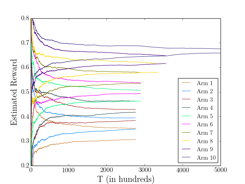
Figure 1: Confidence intervals over time for the lower bound instance outlined in Section 4 for $k=10$. Lines correspond to upper and lower confidence bounds for each arm and cut off at the round in which the arm leaves the active set.

Next, we upper bound the regret of FairBandits.

Theorem 2.

If $\delta<1/\sqrt{T}$, then FairBandits has regret

$$R(T)=O\left(\sqrt{k^{3}T\ln\frac{Tk}{\delta}}\right).$$

Remark 2.

Before proving Theorem 2, we highlight two points. First, this bound becomes non-trivial (i.e. the average per-round regret is $\ll 1$) for $T=\Omega(k^{3})$. As we show in the next section, it is not possible to improve on this. Second, the bound may appear to have suboptimal dependence on $T$ when compared to unconstrained regret bounds (where the dependence on $T$ is often described as logarithmic). However, it is known that $\Omega\left(\sqrt{kT}\right)$ regret is necessary even in the unrestricted setting (without fairness) if one does not make data-specific assumptions on an instance (Bubeck and Cesa-Bianchi, 2012) (e.g. that there is a lower bound on the gap between the best and second best arm). It would be possible to state a logarithmic dependence on $T$ in our setting as well while making assumptions on the gaps between arms, but since our fairness constraint manifests itself as a cost that depends on $k$, we choose for clarity to avoid such assumptions. Without such assumptions, our dependence on $T$ is also optimal.

We now prove Theorem 2. Lemma 2 upper bounds the probability any arm $i$ active in round $t$ has been pulled substantially fewer times than its expectation, i.e. $n_{i}^{t}\ll\frac{t}{k}$. Lemma 3 upper bounds the width of any confidence interval used by FairBandits in round $t$ by $\eta(t)$, conditioned on $i$ being pulled the number of times guaranteed by Lemma 2. Finally, we stitch this together to prove Theorem 2 by upper bounding the total regret incurred for $T$ rounds by noticing that the regret of any arm active in round $t$ is at most $k\eta(t)$.

We begin by lower bounding the probability that any arm active in round $t$ has been pulled substantially fewer times than its expectation.

Lemma 2.

With probability at least $1-\frac{\delta}{2t^{2}}$,

$$n_{i}^{t}\geq\frac{t}{k}-\sqrt{\frac{t}{2}\ln\left(\frac{2k\cdot t^{2}}{\delta}\right)}$$

for all $i\in S^{t}$ (for all active arms in round $t$).

We now use this lower bound on the number of pulls of active arm $i$ in round $t$ to upper-bound $\eta(t)$, an upper bound on the confidence interval width FairBandits uses for any active arm $i$ in round $t$.

Lemma 3.

Consider any round $t$ and any arm $i\in S^{t}$. Condition on $n_{i}^{t}\geq\frac{t}{k}-\sqrt{\frac{t\ln(\frac{2kt^{2}}{\delta})}{2}}$. Then,

$$u_{i}^{t}-\ell_{i}^{t}\leq 2\sqrt{\frac{\ln\left(\left(\pi\cdot t\right)^{2}/3\delta\right)}{2\cdot\frac{t}{k}-\sqrt{\frac{t\ln(\frac{2kt^{2}}{\delta})}{2}}}}=\eta(t).$$

Finally, we prove the bound on the total regret of the algorithm, using the bound on the width of any active arm’s confidence interval in round $t$ provided by Lemma 3.

Proof of Theorem 2.

We condition on $\mu_{i}\in[\ell_{i}^{t},u_{i}^{t}]$ for all $i,t$. This occurs with probability at least $1-\delta$, by Lemma 1. We claim that this implies that arm $i_{*}$ with highest expected reward is always in the active set. This follows from the fact that $\mu_{i_{*}}\in[\ell_{i_{*}}^{t},u_{i_{*}}^{t}]$ and $\mu_{j}\in[\ell_{j}^{t},u_{j}^{t}]$ for all $j,t$; thus, if $\mu_{i_{*}}>\mu_{j}$, it must be that $u_{i_{*}}^{t}\geq\ell_{j}^{t}$. Thus, this holds for $i_{*}^{t}$, the arm with highest upper confidence bound in round $t$, so $i_{*}$ must be chained to $i_{*}^{t}$ in round $t$ for all $t$.

We further condition on the event that for all $j,t$,

$$n_{j}^{t}\geq\frac{t}{k}-\sqrt{\frac{t}{2}\ln\left(\frac{2kt^{2}}{\delta}\right)},$$

which holds with probability at least $1-\frac{\pi\delta}{2}$ by Lemma 2 and a union bound over all times $t$. This implies that, for all rounds $t$, for every active arm $j\in S^{t}$, Lemma 3 applies, and therefore

$$u_{j}^{t}-\ell_{j}^{t}\leq\eta(t).$$

Finally, we upper-bound the per-round regret of pulling any active arm $i\in S^{t}$ at round $t$. Since $i_{*}$ is active, any $i\in S^{t}$ is chained to arm $i_{*}$. Since all active arms have confidence interval width at most $\eta(t)$ and $i$ must be chained using at most $k$ arms’ confidence intervals, we have that

$$\ell_{i}^{t}\geq u_{i_{*}}^{t}-k\cdot\eta(t).$$

Since $\mu_{i}\geq\ell_{i}^{t}$ and $u_{i_{*}}^{t}\geq\mu_{i_{*}}$, it follows that $|\mu_{i}-\mu_{i_{*}}|\leq k\cdot\eta(t)$ for any $i\in S^{t}$. Finally, summing up over all rounds $t\in T$, we know that

$$R(T) \leq\sum_{t:0}^{T}\min(1,k\cdot\eta(t))+\left(1+\frac{\pi}{2}\right)\delta T$$

$$\leq k\left(\sum_{t:\frac{t}{k}>2\sqrt{t\ln\frac{2tk}{\delta}}}^{T}\sqrt{\frac{\ln\frac{t}{\delta}}{\frac{t}{2k}}}+\sum_{t:\frac{t}{k}\leq 2\sqrt{t\ln\frac{2tk}{\delta}}}^{T}1\right)+\left(1+\frac{\pi}{2}\right)\delta T=\tilde{O}(k^{\frac{3}{2}}\sqrt{T\ln\frac{kT}{\delta}}+k^{3})$$

where this bound is derived in Appendix A.1. ∎

4 Fair Classic Stochastic Bandits: A Lower Bound

We now show that the regret bound for FairBandits has an optimal dependence on $k$: no fair algorithm has diminishing regret before $T=\Omega(k^{3})$ rounds. All missing proofs are in Appendix B. The main result of this section is the following.

Theorem 3.

There is a distribution $P$ over $k$-arm instances of the stochastic multi-armed bandit problem such that any fair algorithm run on $P$ experiences constant per-round regret for at least

$$T=\Omega\left(k^{3}\ln\frac{1}{\delta}\right)$$

rounds.

Despite the fact that regret is defined in a prior-free way, the proof of Theorem 3 proceeds via Bayesian reasoning. We construct a family of lower bound instances such that arms have payoffs drawn from Bernoulli distributions, denoted $B(\mu)$ for mean $\mu$. So, to specify a problem instance, it suffices to specify a mean for each of $k$ arms: $\mu_{1},\ldots,\mu_{k}$. The proof formalizes the following outline.

1. We define an instance distribution $P=P_{1}\times\ldots\times P_{k}$ over means $\mu_{i}$ (Definition 3). $P$ will have two important properties. First, we will draw means from $P$ such that for any $i\in[k-1]$, $\mu_{i}=\mu_{i+1}$ with probability at least $1/4$. Second, for any realization of means drawn from $P$, if an algorithm plays uniformly at random over $[k]$, it will suffer constant per-round regret.

2. We treat $P_{i}$ as a prior distribution over mean $\mu_{i}$, and analyze the posterior distribution $P_{i}(r^{1}_{i},,\ldots,r^{t}_{i})$ over means that results after applying Bayes’ rule to the payoff observations $r^{1}_{i},\ldots,r^{t}_{i}$ made by the algorithm. Bayes’ rule implies (Lemma 4) the joint distribution over rewards and means drawn from $P$ is identical to the distribution which first draws means according to $P$, then draws rewards conditioned on those means, and finally resamples the means from the posterior distribution on means. Thus, we can reason about fairness (a frequentist quantity) by analyzing the Bayesian posterior distribution on means conditioned on the observed rewards.

3. A $\delta$-fair algorithm, for any set of means realized from the instance (prior) distribution, must not play arm $i+1$ with lower probability than arm $i$ if $\mu_{i}=\mu_{i+1}$, except with probability $\delta$. By the above change of perspective, therefore, any $\delta$-fair algorithm must play arms $i$ and $i+1$ with equal probability until the posterior distribution on means given observed rewards, satisfies $\mathbb{P}\left[\mu_{i}=\mu_{i+1}|h\right]<\delta$ (Lemmas 5 and 6).

4. We finally lower bound the number of reward observations necessary before the posterior distribution on means given payoffs is such that $\mathbb{P}\left[\mu_{i}=\mu_{i+1}|h\right]<\delta$ for any pair of adjacent arms $i,i+1$. We show that this is $\Omega(k^{2})$ (Lemma 7). Since fair algorithms must play from among the $k$ arms uniformly at random until this point, with high probability, no arm accumulates sufficiently many reward observations until $T=\Omega(k^{3})$ rounds of play.

We begin by describing our distribution over instances. Each arm $i$’s payoff distribution will be Bernoulli with mean $\mu_{i}\sim P_{i}$ independently of each other arm.

Definition 3 (Prior Distribution over $\mu_{i}$).

For each arm $i$, $\mu_{i}$ is distributed according to the distribution with the following probability mass function:

$$P_{i}(x)=\begin{cases}\hfill\frac{1}{2}\hfill&\text{ if $x=\frac{1}{3}+\frac{i}{3k}$}\\ \hfill\frac{1}{2}\hfill&\text{ if $x=\frac{1}{3}+\frac{i+1}{3k}$}.\\ \end{cases}$$

Let $P=\prod_{i}P_{i}$ denote the joint distribution on arms’ expected payoffs.

We treat $P$ as a prior distribution over instances, and analyze the posterior distribution on instances given the realized rewards. Lemma 4 justifies this reasoning.

Lemma 4.

Consider the following two experiments: In the first, let $\mu_{i}\sim P_{i}$ and $r^{1}_{i},\ldots,r^{t}_{i}\sim B(\mu_{i})$, and $W$ denote the joint distribution on $(\mu_{i},r^{1}_{i},\ldots,r^{t}_{i})$. In the second, let $\mu_{i}\sim P_{i}$, and $r^{1}_{i},\ldots,r^{t}_{i}\sim B(\mu_{i})$, and then re-draw the mean $\mu^{\prime}_{i}\sim P_{i}(r^{1}_{i},\ldots,r^{t}_{i})$ from its posterior distribution given the rewards. Let $(\mu^{\prime}_{i},r^{1}_{i},\ldots,r^{t}_{i})\sim W^{\prime}$. Then, $W$ and $W^{\prime}$ are identical distributions.

Next, we lower-bound the number of reward observations necessary such that for some $i\in[k]$: $\mathbb{P}\left[\mu_{i}=\mu_{i+1}|h^{t}\right]<\delta$ with respect to the posterior. It will be useful to refer to an algorithm’s histories as distinguishing the mean of an arm given that history with high probability.

Definition 4 ($\delta$-distinguishing).

We will say $h^{t}$ $\delta$-distinguishes arm $i$ for $\mathcal{A}$ if, for some $\alpha\in[0,1]$,

$$\mathbb{P}_{\mu^{\prime}_{i}\sim P_{i}(h^{t})}\left[\mu^{\prime}_{i}=\alpha\right]\geq 1-\delta.$$

The next lemma shows that if no arm is $\sqrt{\delta}$-distinguished by a history, all pairs of arms $i,i+1$ have posterior probability strictly greater than $\delta$ of having equal means.

Lemma 5.

Suppose $\mathcal{A}$ has history $h^{t}$, and that $h^{t}$ does not $\sqrt{\delta}$-distinguish any arm $i$. Then, for all arms $i,i+1$,

$$\mathbb{P}\left[\mu_{i}=\mu_{i+1}|h^{t}\right]>\delta.$$

Now, we prove that for any fair algorithm, with probability $\geq\tfrac{1}{2}$ over the draw of histories $h^{t}$, $h^{t}$ must $\sqrt{2\delta}$-distinguish some arm, or the algorithm must play uniformly across all $k$ arms conditioned on $h^{t}$.

Lemma 6.

Suppose an algorithm $\mathcal{A}$ is $\delta$-fair. Then:

$$\mathbb{P}_{h^{t}\sim\mathcal{A}}\left[h^{t}\textrm{ does not $\sqrt{2\delta}$-distinguish any $i$}\wedge\exists t^{\prime}\leq t,i\in[k]:\pi^{t^{\prime}}_{i^{\prime}|h^{t^{\prime}}}\neq\frac{1}{k}\right]\leq\frac{1}{2}.$$

We now lower-bound the number of observations from arm $i$ which are required to $\delta$-distinguish it.

Lemma 7.

Fix any $\delta<\frac{1}{8}$. Let $\mu_{i}\sim P_{i}$ as in Definition 3. Then, arm $i$ is $\sqrt{2\delta}$-distinguishable by $h^{t}$ only if $T_{i}=\Omega(k^{2}\ln\frac{1}{\delta})$, where $T_{i}=|\{t^{\prime}:h^{t^{\prime}}_{2}=i,t^{\prime}\leq t\}|$ is the number of times arm $i$ is played.

Proof.

Write $p,p+\frac{1}{3k}$ to represent the two possible realizations that $\mu_{i}$ might take, when drawn from the distribution over instances given in Definition 3. Let $A$ represent the event that $\mu_{i}=p$ and $B$ the event that $\mu_{i}=p+\frac{1}{3k}$. Let $\delta^{\prime}=\sqrt{2\delta}$ throughout.

Fix a history $h^{t}$, and let $m=T_{i}$ represent the number of observations of arm $i$’s reward. We will abuse notation and use $h^{t}_{i}$ to refer to the payoff sequence of arm $i$ observed in history $h^{t}$. $h^{t}_{i}$ is therefore a binary sequence of length $m$; let $||h^{t}_{i}||_{0}=s$ denote the number of $1$s in the sequence. We will calculate conditions under which $h^{t}_{i},m,s$ will imply that either $\frac{1-\delta^{\prime}}{\delta^{\prime}}\leq\frac{\mathbb{P}\left[B|h^{t}_{i}\right]}{\mathbb{P}\left[A|h^{t}_{i}\right]}$ or $\frac{\mathbb{P}\left[B|h^{t}_{i}\right]}{\mathbb{P}\left[A|h^{t}_{i}\right]}\leq\frac{\delta^{\prime}}{1-\delta^{\prime}}$ holds, implying that one of $A$ or $B$ has posterior probability at least $1-\delta^{\prime}$, conditioned on the observed rewards. If neither of these is the case, $i$ is not $\delta^{\prime}$-distinguished by $h^{t}$.

We begin by rearranging our definition of this ratio $X=\frac{\mathbb{P}\left[B|h^{t}_{i}\right]}{\mathbb{P}\left[A|h^{t}_{i}\right]}=\frac{\mathbb{P}\left[h^{t}_{i}|B\right]}{\mathbb{P}\left[h^{t}_{i}|A\right]}$,which follows from Bayes’ rule and the fact that $\mathbb{P}\left[A\right]=\mathbb{P}\left[B\right]$. We wish to upper and lower bound $X$ in terms of $h^{t}_{i}$’s value. By definition of the Bernoulli distribution, we have that

$$X=\frac{\mathbb{P}\left[h^{t}_{i}|B\right]}{\mathbb{P}\left[h^{t}_{i}|A\right]}=\frac{\left(p+\frac{1}{3k}\right)^{s}\left(1-p-\frac{1}{3k}\right)^{m-s}}{\left(p\right)^{s}\left(1-p\right)^{m-s}}=\left(1+\frac{1}{3kp}\right)^{s}\left(1-\frac{1}{3k(1-p)}\right)^{m-s}.$$

We now calculate under what conditions either (a) $X\leq\frac{\delta^{\prime}}{1-\delta^{\prime}}$, or (b) $X\geq\frac{1-\delta^{\prime}}{\delta^{\prime}}$. One of these must hold if $i$ is $\delta^{\prime}$-distinguished. Before we do so, we mention that a Chernoff bound implies that with probability $1-\delta^{\prime}$, for events $A$ and $B$, Equations 1 and 2, respectively:

$$|s-mp|\leq\sqrt{2m\ln\frac{2}{\delta^{\prime}}}$$ (1)

$$|s-mp-\frac{m}{3k}|\leq\sqrt{2m\ln\frac{2}{\delta^{\prime}}}$$ (2)

since the mean of $m$ Bernoulli trials with mean $p$ ( or $p+\frac{1}{3k}$) is $mp$ (or $mp+\frac{m}{3k}$).

We begin by analyzing case (a), where $\delta^{\prime}=\sqrt{2\delta}<1/2$ implies

$$2\delta^{\prime}>\frac{\delta^{\prime}}{1-\delta^{\prime}}\geq X=\left(1+\frac{1}{3kp}\right)^{s}\left(1-\frac{1}{3k(1-p)}\right)^{m-s}.$$

Taking logarithms on both sides, we have that

$$\ln(2\delta^{\prime})>s\ln\left(1+\frac{1}{3kp}\right)+(m-s)\ln\left(1-\frac{1}{3k(1-p)}\right)\geq s\frac{1}{3kp+1}-(m-s)\frac{1}{3k(1-p)-1}$$

where the inequality follows from $\ln(1+x)\geq\frac{x}{x+1}$ for $x\in[-1,\infty]$. Then, this implies that

$$(3kp+1)(3k(1-p)-1)\ln(2\delta^{\prime}) >s(3k(1-p)-1)-(m-s)(3kp+1) =3ks-3kpm-m.$$

Multiplying both sides by $-1$, this implies that

$$(3kp+1)(3k(1-p)-1)\ln\frac{1}{2\delta^{\prime}}<m+3kpm-3ks.$$

Equation 1 implies $|3ks-3kmp-m|\leq m+3k\sqrt{2m\ln\frac{2}{\delta^{\prime}}}$, which with the previous line implies

$$(3kp+1)(3k(1-p)-1)\ln\frac{1}{2\delta^{\prime}}<m+3k\sqrt{2m\ln\frac{2}{\delta^{\prime}}}.$$

Since $p,1-p\in[1/3,2/3]$ and $\delta^{\prime}=\sqrt{2\delta}$, solving for $m$ implies that $m=\Omega(k^{2}\ln\frac{1}{\delta^{\prime}})$.

In case (b), we have

$$\frac{1}{2\delta^{\prime}}<\frac{1-\delta^{\prime}}{\delta^{\prime}}\leq X=\left(1+\frac{1}{3kp}\right)^{s}\left(1-\frac{1}{3k(1-p)}\right)^{m-s}\leq e^{\frac{s}{3kp}}e^{\frac{-(m-s)}{3k(1-p)}}$$

where we used the fact that $1+x\leq e^{x}$ for all $x$. Taking logarithms, this will imply that

$$\frac{s}{3kp}-\frac{m-s}{3k(1-p)}>\ln\frac{1}{2\delta^{\prime}}\Rightarrow s-mp=s(1-p)-(m-s)p>3kp(1-p)\ln\frac{1}{2\delta^{\prime}}\geq\frac{6k}{9}\ln\frac{1}{2\delta^{\prime}}$$ (3)

whose last inequality comes the range of $p$. Combining this inequality with Equation 2, this implies

$$\sqrt{2m\ln\frac{1}{2\delta^{\prime}}}+\frac{m}{k}>\frac{6k}{9}\ln\frac{1}{2\delta^{\prime}}$$

and solving for $m$ and substituting for $\delta^{\prime}$ gives that $m=\Omega(k^{2}\ln\frac{1}{\delta})$.

Thus, if either $X\geq\frac{1-\delta^{\prime}}{\delta^{\prime}}$ or $X\leq\frac{\delta^{\prime}}{1-\delta^{\prime}}$, it must be that $m=\Omega(k^{2}\ln\frac{1}{\delta})$. ∎

We now have the tools in hand to prove Theorem 3.

Proof of Theorem 3.

Assume $\mathcal{A}$ is some $\delta$-fair algorithm where $\delta<1/8$. Fix $T$; we claim that with probability at least $\frac{1}{2}$, for any $t=o(k^{3}\ln\frac{1}{\delta})$, $t\leq T$, $\pi^{t}_{j|h^{t}}=\frac{1}{k}$ for all $j$. Since the payoff for uniformly random play is $\leq\frac{1}{2}+\frac{1}{k}$, while the best arm has payoff $\geq\frac{2}{3}$, in any round $t$ where $\pi^{t}_{i|h^{t}}=\pi^{t}_{i^{\prime}|h^{t}}$ for all $i,i^{\prime}\in[k]$, the algorithm suffers $\Omega(1)$ regret in that round.

Lemma 6 implies that, with probability at least $\frac{1}{2}$ over the distribution over histories $h^{t}$, either (a) $\pi^{t^{\prime}}_{i|h^{t^{\prime}}}=\pi^{t^{\prime}}_{i^{\prime}|h^{t^{\prime}}}$ for all $i,i^{\prime}\in[k],t^{\prime}\leq t$ or (b) $h^{t}$ must $\sqrt{2\delta}$-distinguish some arm $i$. Case $(a)$ implies our claim. In case (b), Lemma 7 states than an arm $i$ is $\sqrt{2\delta}$-distinguishable only if $T_{i}=\Omega(k^{2}\ln\frac{1}{\delta})$. We now argue that unless $t=\Omega(k^{3}\ln\frac{1}{\delta})$, $T_{i}=o(k^{2}\ln\frac{1}{\delta})$, which will imply our claim for case $(b)$.

Fix some $i,t$. We lower-bound $t$ for which, with probability at least $1-\frac{\delta^{\prime}}{k}$ over histories $h^{t}$, it will be the case that $n_{i}^{t}\geq c\cdot k^{2}\ln\frac{1}{\delta}$ when $\pi^{t^{\prime}}_{i|h^{t^{\prime}}}=\pi^{t^{\prime}}_{i^{\prime}|h^{t^{\prime}}}$ for all $i,i^{\prime}\in[k],t^{\prime}\leq t$. Let $X_{1},\ldots,X_{t}$ be indicator variables of arm $i$ being played in round $t^{\prime}\leq t$. Note that for all $t^{\prime}\leq t$, $E[X_{t^{\prime}}]=\frac{1}{k}$, since in all rounds prior to $t$, we have all arms are played with equal probability. For any $\epsilon\in[0,1]$, as $n_{i}^{t^{\prime}}$ are nondecreasing in $t^{\prime}$, an additive Chernoff bound implies

$$\mathbb{P}\left[\exists t^{\prime}\leq t:n_{i}^{t^{\prime}}\geq\frac{t}{k}+\epsilon t\right]\leq\mathbb{P}\left[\sum_{t^{\prime}\leq t}X_{t^{\prime}}>\frac{t}{k}+\epsilon t\right]\leq e^{-2t\epsilon^{2}}$$

which, for $\epsilon t=\sqrt{\frac{t\ln\frac{2k}{\delta^{\prime}}}{2}}$, becomes $\mathbb{P}\left[\sum_{t^{\prime}\leq t}X_{t^{\prime}}>\frac{t}{k}+\epsilon t\right]\leq\frac{\delta^{\prime}}{k}.$ So, using a union bound over all $k$ arms, with probability $1-\delta^{\prime}$, for some fixed $t$ and all $i$, $n_{i}^{t}\leq\frac{t}{k}+\sqrt{\frac{t\ln\frac{2k}{\delta^{\prime}}}{2}}$. We condition on the event that $n_{i}^{t}$ satisfies this inequality for a fixed $t$ and all $i$. If $n_{i}^{t}\geq c\cdot k^{2}\ln\frac{1}{\delta}$, this implies

$$\frac{t}{k}+\sqrt{\frac{t\ln\frac{2k}{\delta^{\prime}}}{2}}\geq c\cdot k^{2}\ln\frac{1}{\delta}\quad\Rightarrow\quad t\geq-k\sqrt{\frac{t\ln\frac{2k}{\delta^{\prime}}}{2}}+c\cdot k^{3}\ln\frac{1}{\delta}.$$

If $k\sqrt{\frac{t\ln\frac{2k}{\delta^{\prime}}}{2}}\leq\frac{c}{2}\cdot k^{3}\ln\frac{1}{\delta}$, then $t\geq\frac{c}{2}\cdot k^{3}\ln\frac{1}{\delta}$; if not, then $t\geq\frac{\frac{c^{2}}{2}k^{4}\ln^{2}\frac{1}{\delta}}{\ln\frac{2k}{\delta^{\prime}}}$. Thus, $n_{i}^{t}<c\cdot k^{2}\ln\frac{1}{\delta}$ with probability $1-\delta^{\prime}$ for all $i$ unless $t\geq\min\left(\frac{c}{2}\cdot k^{3}\ln\frac{1}{\delta},\frac{\frac{c^{2}}{2}k^{4}\ln^{2}\frac{1}{\delta}}{\ln\frac{2k}{\delta^{\prime}}}\right)=\Omega(k^{3}\ln\frac{1}{\delta})$ for $\delta^{\prime}\in[\frac{1}{2},1]$. ∎

5 KWIK Learnability Implies Fair Bandit Learnability

In this section, we show if a class of functions is KWIK learnable, then there is a fair algorithm for learning the same class of functions in the contextual bandit setting, with a regret bound polynomially related to the function class’ KWIK bound. Intuitively, KWIK-learnability of a class of functions guarantees we can learn the function’s behavior to a high degree of accuracy with a high degree of confidence. As fairness constrains an algorithm most before the algorithm has determined the payoff functions’ behavior accurately, this guarantee enables us to learn fairly without incurring much additional regret. Formally, we prove the following polynomial relationship.

Theorem 4.

For an instance of the contextual multi-armed bandit problem where $f_{j}\in C$ for all $j\in[k]$, if $C$ is $(\epsilon,\delta)$-KWIK learnable with bound $m(\epsilon,\delta)$, KWIKToFair $(\delta,T)$ is $\delta$-fair and achieves regret bound:

$$R(T)=O\left(\max\left(k^{2}\cdot m\left(\epsilon^{*},\frac{\min\left(\delta,1/T\right)}{T^{2}k}\right),k^{3}\ln\frac{k}{\delta}\right)\right)$$

for $\delta\leq\frac{1}{\sqrt{T}}$ where $\epsilon^{*}=\arg\min_{\epsilon}(\max(\epsilon\cdot T,k\cdot m(\epsilon,\frac{\min(\delta,1/T)}{kT^{2}}))).$

First, we construct an algorithm KWIKToFair$(\delta,T)$ that uses the KWIK learning algorithm as a subroutine, and prove that it is $\delta$-fair. A call to KWIKToFair$(\delta,T)$ will initialize a KWIK learner for each arm, and in each of the $T$ rounds will implicitly construct a confidence interval around the prediction of each learner. If a learner makes a numeric valued prediction, we will interpret this as a confidence interval centered at the prediction with width $\epsilon^{*}$. If a learner outputs $\bot$, we interpret this as a trivial confidence interval (covering all of $[0,1]$). We use the same chaining technique that we use in the classic stochastic setting. In every round $t$, KWIKToFair $(\delta,T)$ identifies the arm $i_{*}^{t}=\operatorname*{arg\,max}_{i}u_{i}^{t}$ that has the largest upper confidence bound. At each round $t$, we will say $i$ is linked to $j$ if $[\ell_{i}^{t},u_{i}^{t}]\cap[\ell_{j}^{t},u_{j}^{t}]\neq\emptyset$, and $i$ is chained to $j$ if they are in the same component of the transitive closure of the linked relation. Then, it plays uniformly at random amongst all arms chained to arm $i_{*}^{t}$. Whenever all learners output predictions, they need no feedback. When a learner for $j$ outputs $\bot$, if $j$ is selected then we have feedback $r^{t}_{j}$ to give it; on the other hand, if $j$ isn’t selected, we “roll back” the learning algorithm for $j$ to before this round by not updating the algorithm’s state.

1:procedure KWIKToFair($\delta,T$)

2:     $\delta^{*}\leftarrow\frac{\min(\delta,\frac{1}{T})}{kT^{2}}$, $\epsilon^{*}\leftarrow\arg\min_{\epsilon}(\max(\epsilon\cdot T,k\cdot m(\epsilon,\delta^{*})))$

3:     Initialize KWIK$(\epsilon^{*},\delta^{*})$-learner $L_{i}$, $h_{i}\leftarrow[\,]$ $\forall i\in[k]$

4:     for $1\leq t\leq T$ do

5:         S $\leftarrow\emptyset$ $\triangleright$ Initialize set of predictions $S$

6:         for $i=1,\ldots,k$ do

7:              $s^{t}_{i}\leftarrow L_{i}(x_{i}^{t},h_{i})$

8:              $S\leftarrow S\cup s^{t}_{i}$ $\triangleright$ Store prediction $s^{t}_{i}$          

9:         if $\perp\in S$ then

10:              Pull $j^{*}\leftarrow(x\in_{R}[k])$, receive reward $r^{t}_{j^{*}}$ $\triangleright$ Pick arm at random from all arms

11:         else

12:              $i_{*}^{t}\leftarrow\arg\max_{i}s^{t}_{i}$

13:              $S^{t}\leftarrow\{j\mid(s^{t}_{j}-\epsilon^{*},s^{t}_{j}+\epsilon^{*})\text{ chains to }(s^{t}_{i_{*}^{t}}-\epsilon^{*},s^{t}_{i_{*}^{t}}+\epsilon^{*})\}$

14:              Pull $j^{*}\leftarrow(x\in_{R}S^{t})$, receive reward $r^{t}_{j^{*}}$ $\triangleright$ Pick arm at random from active set $s^{t}_{i^{*}}$          

15:         $h_{j^{*}}\leftarrow h_{j^{*}}::(x_{{j^{*}}}^{t},r^{t}_{j^{*}})$ $\triangleright$ Update the history for $L_{j^{*}}$      

We begin by bounding the probability of certain failures of KWIKToFair in Lemma 8, proven in Appendix C. This in turn lets us prove the fairness of KWIKToFair in Theorem 5.

Lemma 8.

With probability at least $1-\min(\delta,\frac{1}{T})$, for all rounds $t$ and all arms $i$, (a) if $s^{t}_{i}\in\mathbb{R}$ then $|s^{t}_{i}-f_{i}(x^{t}_{i})|\leq\epsilon^{*}$ and (b) $\sum_{t}\mathbb{I}\left[s^{t}_{i}=\bot\text{ and $i$ is pulled}\right]\leq m(\epsilon^{*},\delta^{*})$.

Theorem 5.

KWIKToFair$(\delta,T)$ is $\delta$-fair.

Proof of Theorem 5.

We condition on both (a) and (b) holding for all arms $i$ and rounds $t$ from Lemma 8, which occur with probability $1-\delta$ for all arms and all times $t$. Therefore, we proceed by conditioning on the event that for all arms $i$ and all rounds $t$, if $L_{i}=s^{t}_{i}$ for $s^{t}_{i}\neq\bot$ then $|s^{t}_{i}-f_{i}(x^{t}_{i})|\leq\epsilon^{*}$. Having done so, there are two possibilities for each round $t$.

In case 1, for each $i$ we have that $L_{i}(x^{t}_{i})=s^{t}_{i}\neq\bot$. By the condition above, for any arms $i$ and $j$, $f_{i}(x_{i}^{t})\geq f_{j}(x_{j}^{t})$ implies that $s^{t}_{i}+\epsilon^{*}\geq s^{t}_{j}-\epsilon^{*}$. Since in this case no learner outputs $\bot$, arm $j$ chains to the top arm only if arm $i$ does. Therefore $\pi_{i\mid h}^{t}\geq\pi_{j\mid h}^{t}$. In case 2, there exists some $i$ such that $L_{i}(x^{t}_{i})=\bot$. Then we choose uniformly at random across all arms, so $\pi_{i\mid h}^{t}=\pi_{j\mid h}^{t}$ for all $i$ and $j$.

Thus, with probability at least $1-\delta$, for each round $t$, $f_{i}(x_{i}^{t})\geq f_{j}(x_{j}^{t})$ implies that $\pi_{i\mid h}^{t}\geq\pi_{j\mid h}^{t}$. ∎

We now use the KWIK bounds of the KWIK learners to upper-bound the regret of KWIKToFair$(\delta,T)$.

Lemma 9.

KWIKToFair$(\delta,T)$ achieves regret $O(\max(k^{2}\cdot m(\epsilon^{*},\delta^{*}),k^{3}\ln\frac{Tk}{\delta}))$.

Proof.

We first condition on the event that both (a) and (b) from Lemma 8 hold for all $t,i$, which holds with probability $1-\min(\delta,\frac{1}{T})$, and bound the regret when they both hold. Choose an arbitrary round $t$ in the execution of KWIKToFair$(\delta,T)$. As above, there are two cases. In the first case, $L_{i}(x^{t}_{i})=s^{t}_{i}\neq\bot$ for all $i$ and we choose uniformly at random from the arms chained by $\epsilon^{*}$-intervals to the arm with the highest prediction. Since we have conditioned on the event that all KWIK learners are correct, $i^{*}\in S^{t}$. Furthermore, for any $i,j\in S^{t}$, we have that $|s^{t}_{i}-s^{t}_{j}|\leq 2k\epsilon^{*}$, and in particular that $|s^{t}_{i}-s^{t}_{i^{*}}|\leq 2k\epsilon^{*}$. Thus, the regret is at most $2k\epsilon^{*}$ in such a round. In the second case some arm outputs $\bot$, so we choose randomly from all $k$ arms, and the worst-case regret is 1. Thus, the total regret will be at most $2k\epsilon^{*}T+n+\delta T$ where $n$ is the number of rounds in which some $L_{i}$ outputs $\bot$.

We now upper bound $n_{i}$, the number of rounds in which arm $i$ outputs $\bot$. Fix some arm $i$ which outputs $\bot$ in $n_{i}$ rounds. Arm $i$ is played and therefore receives feedback every time it outputs $\bot$ with probability at least $1/k$. Thus, using a Chernoff bound, with probability $1-\delta^{\prime}$, arm $i$ receives feedback for $n_{i}$ outputs of $\bot$ in at least $\frac{n_{i}}{k}-\sqrt{2n_{i}\ln\frac{2}{\delta^{\prime}}}$ rounds. $L_{i}$ has the guarantee that there can be at most $m(\epsilon^{*},\delta^{*})$ many such rounds (in which it outputs $\bot$ and receives feedback). Thus,

$$m(\epsilon^{*},\delta^{*})\geq\frac{n_{i}}{k}-\sqrt{2n_{i}\ln\frac{2}{\delta^{\prime}}}.$$

If $n_{i}\geq ck\cdot m(\epsilon^{*},\delta^{*})$, this implies

$$m(\epsilon^{*},\delta^{*})\geq c\cdot m(\epsilon^{*},\delta^{*})-\sqrt{2ck\cdot m(\epsilon^{*},\delta^{*})\ln\frac{2}{\delta^{\prime}}}.$$

We now analyze cases in which (1) $k\ln\frac{2}{\delta^{\prime}}\leq m(\epsilon^{*},\delta^{*})$ and (2) $k\ln\frac{2}{\delta^{\prime}}>m(\epsilon^{*},\delta^{*})$.

Case (1) this implies

$$m(\epsilon^{*},\delta^{*})\geq c\cdot m(\epsilon^{*},\delta^{*})-\sqrt{2c}\cdot m(\epsilon^{*},\delta^{*}).$$

For $c>4$, this leads to contradiction. Thus, in this case, if we set $\delta^{\prime}=\frac{\delta}{k}$, we know that with probability $1-\delta$, $n_{i}\leq 4k\cdot m(\epsilon^{*},\delta^{*})$ which summing up over all $i$ implies $\sum_{i}n_{i}\leq 4k^{2}\cdot m(\epsilon^{*},\delta^{*})$, as desired.

In case (2), we have that

$$\ln\frac{2}{\delta^{\prime}}\geq\frac{n_{i}}{k}-\sqrt{2n_{i}\ln\frac{2}{\delta^{\prime}}}$$

which solving for $n_{i}$ implies that $n_{i}=O(k^{2}\ln\frac{1}{\delta^{\prime}})$, so $\sum_{i}n_{i}=O(k^{3}\ln\frac{k}{\delta})$ by setting $\delta^{\prime}=\frac{\delta}{k}$ and taking a union bound. Thus, there are at most $n=O(\max(k^{2}\cdot m(\epsilon,\delta^{*}),k^{3}\ln\frac{k}{\delta}))$ rounds in expectation during the execution of KWIKToFair$(\delta,T)$ in which some arm outputs $\bot$.

Combining both cases, the total regret incurred by KWIKToFair$(\delta,T)$ across all $T$ rounds is

$$R(T)=4k^{2}\cdot m(\epsilon^{*},\delta^{*})+k^{3}\ln\left(\frac{k}{\delta}\right)+T\cdot 2k\epsilon^{*}+T\cdot\min(\delta,\frac{1}{T})=O(\max(k^{2}\cdot m(\epsilon^{*},\delta^{*}),k^{3}\ln\frac{k}{\delta})).$$

∎

Our presentation of KWIKToFair$(\delta,T)$ has a known time horizon $T$. Its guarantees extend to the case in which $T$ is unknown via the standard “doubling trick” to prove Theorem 4 in Appendix C.

An important instance of the contextual bandit problem is the linear case, where $C$ consists of the set of all linear functions of bounded norm in $d$ dimensions. This captures the natural setting in which the rewards of each arm are governed by an underlying linear regression model on a $d$-dimensional real valued feature space. The linear case is well studied, and there are known KWIK algorithms (Strehl and Littman, 2008) for the set of linear functions $C$, which allows us via our reduction to give a fair contextual bandit algorithm for this setting with a polynomial regret bound.

Lemma 10 ((Strehl and Littman, 2008)).

Let $C=\{f_{\theta}|f_{\theta}(x)=\langle\theta,x\rangle,\theta\in\mathbb{R}^{d},||\theta||\leq 1\}$ and $\mathcal{X}=\{x\in\mathbb{R}^{d}:||x||\leq 1\}$. $C$ is KWIK learnable with KWIK bound $m(\epsilon,\delta)=\tilde{O}(d^{3}/\epsilon^{4})$.

Then, an application of Theorem 4 implies that KWIKToFair has a polynomial regret guarantee for the class of linear functions. This proof can be found in Appendix C.

Corollary 1.

Let $C$ and $\mathcal{X}$ be as in Lemma 10, and $f_{j}\in C$ for each $j\in[k]$. Then, KWIKToFair$(T,\delta)$ using the learner from (Strehl and Littman, 2008) has regret:

$$R(T)=\tilde{O}\left(\max\left(T^{4/5}k^{6/5}d^{3/5},k^{3}\ln\frac{k}{\delta}\right)\right).$$

6 Fair Bandit Learnability Implies KWIK Learnability

In this section, we show how to use a fair, no-regret contextual bandit algorithm to construct a KWIK learning algorithm whose KWIK bound has logarithmic dependence on the number of rounds $T$. Intuitively, any fair algorithm which achieves low regret must both be able to find and exploit an optimal arm (since the algorithm is no-regret) and can only exploit that arm once it has a tight understanding of the qualities of all arms (since the algorithm is fair). Thus, any fair no-regret algorithm will ultimately have tight $(1-\delta)$-confidence about each arm’s reward function.

Theorem 6.

Suppose $\mathcal{A}$ is a $\delta$-fair algorithm for the contextual bandit problem over the class of functions $C$, with regret bound $R(T,\delta)$. Suppose also there exists $f\in C,x(\ell)\in\mathcal{X}$ such that for every $\ell\in[\lceil\frac{1}{\epsilon}\rceil]$, $f(x(\ell))=\ell\cdot\epsilon$. Then, FairToKWIK is an $(\epsilon,\delta)$-KWIK algorithm for $C$ with KWIK bound $m(\epsilon,\delta)$, with $m(\epsilon,\delta)$ the solution to $\frac{m(\epsilon,\delta)\epsilon}{4}=R(m(\epsilon,\delta),\frac{\epsilon\delta}{2T})$.

Remark 3.

The condition that $C$ should contain a function that can take on values that are multiples of $\epsilon$ is for technical convenience; $C$ can always be augmented by adding a single such function.

Our aim is to construct a KWIK algorithm $\mathcal{B}$ to predict labels for a sequence of examples labeled with some unknown function $f^{*}\in C$. To do this, we will run our fair contextual bandit algorithm $\mathcal{A}$ on an instance that we construct online as examples $x^{t}$ arrive for $\mathcal{B}$. The idea is to simulate a two arm instance, in which one arm’s rewards are governed by $f^{*}$ (the function to be KWIK learned), and the other arm’s rewards are governed by a function $f$ that we can set to take any value in $\{0,\epsilon,2\epsilon,\ldots,1\}$. For each input $x^{t}$, we perform a thought experiment and consider $\mathcal{A}$’s probability distribution over arms when facing a context which forces arm $2$’s payoff to take each of the values $0,\epsilon^{*},2\epsilon^{*},\ldots,1$. Since $\mathcal{A}$ is fair, $\mathcal{A}$ will play arm $1$ with weakly higher probability than arm $2$ for those $\ell:\ell\epsilon^{*}\leq f(x^{t})$; analogously, $\mathcal{A}$ will play arm $1$ with weakly lower probability than arm $2$ for those $\ell:\ell\epsilon^{*}\geq f(x^{t})$. If there are at least $2$ values of $\ell$ for which arm $1$ and arm $2$ are played with equal probability, one of those contexts will force $\mathcal{A}$ to suffer $\epsilon^{*}$ regret, so we continue the simulation of $\mathcal{A}$ on one of those instances selected at random, forcing at least $\epsilon^{*}/2$ regret in expectation, and at the same time have $\mathcal{B}$ return $\bot$. $\mathcal{B}$ receives $f^{*}(x^{t})$ on such a round, which is used to construct feedback for $\mathcal{A}$. Otherwise, $\mathcal{A}$ must transition from playing arm $1$ with strictly higher probability to playing $2$ with strictly higher probability as $\ell$ increases: the point at which that occurs will “sandwich” the value of $f(x^{t})$, since $\mathcal{A}$’s fairness implies this transition must occur when the expected payoff of arm $2$ exceeds that of arm $1$. $\mathcal{B}$ uses this value to output a numeric prediction.

An important fact we exploit is that we can query $\mathcal{A}$’s behavior on $(x^{t},x(\ell))$, for any $x^{t}$ and $\ell\in\left[\lceil\frac{1}{\epsilon^{*}}\rceil\right]$ without providing it feedback (and instead “roll back” its history to $h^{t}$ not including the query $(x^{t},x(\ell))$). We update $\mathcal{A}$’s history by providing it feedback only in rounds where $\mathcal{B}$ outputs $\bot$.

1:procedure FairToKWIK($\epsilon,\delta,T$)

2:     $\epsilon^{*}\leftarrow\frac{\epsilon}{2}$, $\delta^{*}\leftarrow\frac{\delta\cdot\epsilon^{*}}{T}$, $h\leftarrow[\,]$, initialize fair $\mathcal{A}(\delta^{*},T)$ for class $C$

3:     for $1\leq t\leq T$ do

4:         $h^{t}\leftarrow h$

5:         for $\ell\in\left[\lceil\frac{1}{\epsilon^{*}}\rceil\right]$ do

6:              Let $(p^{t,\ell}_{1},p^{t,\ell}_{2})=(\pi_{1|h^{t}},\pi_{2|h^{t}}))$ be $\mathcal{A}(h^{t},(x^{t},x(\ell)))$’s dist. over arms given $h$          

7:         if $\exists\ell\neq\ell^{\prime}:\ell,\ell^{\prime}\in\left[\lceil\frac{1}{\epsilon^{*}}\rceil\right]$: $p^{t,{\ell}}_{1}=p^{t,{\ell}}_{2}=p^{t,{\ell^{\prime}}}_{1}=p^{t,{\ell^{\prime}}}_{2}$ then

8:

9:              Choose $x(\hat{\ell})\in_{R}\{x(\ell),x(\ell^{\prime})\}$ $\triangleright$ One of $x(\ell),x(\ell^{\prime})$ must cause $\epsilon^{*}$ regret

10:              Select $a^{t}\sim\mathcal{A}(h^{t},(x^{t},x(\hat{\ell})))$ $\triangleright$ Run $\mathcal{A}$ to get a predicted arm

11:              Predict $\hat{y}^{t}\leftarrow\bot$

12:              if $a^{t}=1$ then

13:                  $r^{t}_{1}\leftarrow y^{t}$ and $h\leftarrow h^{t}::((x^{t},x(\hat{\ell})),1,r^{t}_{1})$ $\triangleright$ Use KWIK feedback

14:              else

15:                  $r^{t}_{2}\leftarrow\hat{\ell}\epsilon^{*}$

16:                  $h\leftarrow h^{t}::((x^{t},x(\hat{\ell})),2,r^{t}_{2})$ $\triangleright$ Construct feedback for arm $2$               

17:         else$\triangleright$ $\mathcal{A}$’s history is not updated

18:              if $p^{t,\ell}_{1}\leq p^{t,\ell}_{2}$ for all $\ell\in\left[\lceil\frac{1}{\epsilon^{*}}\rceil\right]$ then

19:                  $\hat{\ell}\leftarrow 0$

20:              else Let $\hat{\ell}$ be the largest index for which $p^{t,\hat{\ell}}_{1}>p^{t,\hat{\ell}}_{2}$               

21:              Predict $\hat{y}^{t}\leftarrow\hat{\ell}\cdot\epsilon^{*}$               

Proof.

For a fixed run of $\mathcal{A}$, we calculate the probability that for all times $t$ and $\ell\in\left[\lceil\frac{1}{\epsilon^{*}}\rceil\right]$, it is the case that $p^{t,\ell}_{1}>p^{t,\ell}_{2}$ only if $f^{*}(x^{t})>\ell\cdot\epsilon^{*}$ and also $p^{t,\ell}_{1}<p^{t,\ell}_{2}$ only if $f^{*}(x^{t})<\ell\cdot\epsilon^{*}$. In this run, $\mathcal{A}$ is queried on $\frac{T}{\epsilon^{*}}$ histories and contexts: prefixes of $h$ along with $(x^{t},x(\ell))$ for each $t\in[T],\ell\in\left[\lceil\frac{1}{\epsilon^{*}}\rceil\right]$. The fairness of $\mathcal{A}$ implies for any fixed $h^{t}$ and fixed $(x^{t},x(\ell))$, with probability $1-\delta^{*}$, $p^{t,\ell}_{1}>p^{t,\ell}_{2}$ only if $f^{*}(x^{t})>\ell\epsilon^{*}$ and $p^{t,\ell}_{1}<p^{t,\ell}_{2}$ only if $f^{*}(x^{t})<\ell\epsilon^{*}$. Then, by a union bound over $t\in[T],\ell\in\left[\lceil\frac{1}{\epsilon^{*}}\rceil\right]$, with probability at least $1-\delta^{*}\frac{T}{\epsilon^{*}}=1-\delta$, $\mathcal{A}(h^{t},x^{t},x(\ell))$ will satisfy this property for all $t\in[T],\ell\in\left[\lceil\frac{1}{\epsilon^{*}}\rceil\right]$. We condition on this holding in the remainder of the proof.

We now argue that the numeric predictions of $\mathcal{B}$ are correct within an additive $\epsilon$. Let:

$$E^{t}=\{\ell:p^{t,\ell}_{1}=p^{t,\ell}_{2}\}.$$

When $\mathcal{B}(x^{t})=y^{t}\in[0,1]$, note that $|E^{t}|\leq 1$, else $\mathcal{B}$ would have output $\bot$.

If $p^{t,\ell}_{1}\leq p^{t,\ell}_{2}$ for all $\ell$, since $|E^{t}|\leq 1$, either $p^{t,0}_{1}<p^{t,0}_{2}$ or $p^{t,1}_{1}<p^{t,1}_{2}$, which we have conditioned on implying that either $f^{*}(x^{t})<f(x(0))=0$ or $f^{*}(x^{t})<f(x(1))=\epsilon^{*}$. Since $f^{*}(x^{t})\geq 0$, this implies $f^{*}(x^{t})\in[0,\epsilon^{*})=[\hat{\ell}\epsilon^{*},\epsilon^{*})=[\hat{y}^{t},\hat{y}^{t}+\epsilon^{*})$.

Otherwise, we have that $p^{t,\hat{\ell}}_{1}>p^{t,\hat{\ell}}_{2}$, and $p^{t,\ell}_{1}\leq p^{t,\ell}_{2}$ for all $\ell>\hat{\ell}$. If $(a)$ $\hat{\ell}=\lceil\frac{1}{\epsilon^{*}}\rceil$, then $f^{*}(x^{t})>1$, a contradiction, so $\hat{\ell}<\lceil\frac{1}{\epsilon^{*}}\rceil$. If $(b)$ $\hat{\ell}=\lceil\frac{1}{\epsilon^{*}}\rceil-1$, then $f^{*}(x^{t})>f(x(\hat{\ell}))=(\lceil\frac{1}{\epsilon^{*}}\rceil-1)\epsilon^{*}$ and so $f^{*}(x^{t})\in((\lceil\frac{1}{\epsilon^{*}}\rceil-1)\epsilon^{*},1]=(\hat{y^{t}},\hat{y}^{t}+\epsilon^{*}]$, so $\hat{y^{t}}$ is $\epsilon^{*}$-accurate. If neither $(a)$ nor $(b)$, then $(c)$ it must be $\hat{\ell}<\lceil\frac{1}{\epsilon^{*}}\rceil-1$. Since $|E^{t}|\leq 1$, for some $\ell\in\{\hat{\ell}+1,\hat{\ell}+2\}$, we know that $p^{t,\ell}_{1}<p^{t,\ell}_{2}$; thus, $f^{*}(x^{t})<f(x(\ell))\leq(\hat{\ell}+2)\epsilon^{*}$ and therefore $f^{*}(x^{t})\in(\hat{\ell}\epsilon^{*},(\hat{\ell}+2)\epsilon^{*})=(\hat{y}^{t},\hat{y}^{t}+2\epsilon^{*})$.

Finally, we upper-bound $m(\epsilon,\delta)$, the number of rounds $t:\mathcal{B}(x^{t})=\bot$. For each such $t$, $\mathcal{A}$ runs on a random draw of one of two contexts, one of whose arms’ payoffs differ by at least $\epsilon^{*}$. Thus, for one of those contexts, either $f^{*}(x^{t})\geq f(x)-\epsilon^{*}$ or $f^{*}(x^{t})\leq f(x)-\epsilon^{*}$. In either case, since $p^{t,\ell}_{1}=p^{t,\ell}_{2}=\frac{1}{2}$ for $x(\ell)=x$, $\mathcal{A}$ suffers expected regret at least $\frac{\epsilon^{*}}{2}$ for that context, and at least $\frac{\epsilon^{*}}{4}$ when faced with one chosen at random. Thus, $m(\epsilon,\delta)\cdot\frac{\epsilon^{*}}{4}=m(\epsilon,\delta)\cdot\frac{\epsilon}{8}<R(m(\epsilon,\delta),\delta^{*})=R(m(\epsilon,\delta),\frac{\epsilon\delta}{2T})$, since $\mathcal{A}$’s regret is upper bounded by this quantity over $m(\epsilon,\delta)$ rounds (which is an upper bound on the number of rounds for which $\mathcal{A}$ is actually run and updated). ∎

6.1 An Exponential Separation Between Fair and Unfair Learning

In this section, we exploit the other direction of the equivalence we have proven between fair contextual bandit algorithms and KWIK learning algorithms to give a simple contextual bandit problem for which fairness imposes an exponential cost in its regret bound. This is in contrast to the case in which the underlying class of functions is linear, for which we gave fair contextual bandit algorithms with regret bounds within a polynomial factor of their unconstrained counterparts. In this problem, the context domain is the $d$-dimensional boolean hypercube: $\mathcal{X}=\{0,1\}^{d}$ – i.e. the context each round for each individual consists of $d$ boolean attributes. Our class of functions $C$ is the class of boolean conjunctions:

$$C=\{f\mid f(x)=x_{i_{1}}\wedge x_{i_{2}}\wedge\ldots\wedge x_{i_{k}}\text{ where }0\leq k\leq d\text{ and }i_{1},\ldots,i_{k}\in[d]\}.$$

We first give a simple but unfair algorithm, ConjunctionBandit, for this problem which obtains a regret bound which is linear in $d$. It maintains a set of candidate variables $C_{j}^{*}$ for each conjunction $f_{j}$; this set shrinks across rounds, while always containing the true set of variables over which $f_{j}$ is defined. We denote the boolean value of variable $m$ in the context for arm $j$ in round $t$ by $x_{j,m}^{t}$.

The formal claim and proof that ConjunctionBandit achieves regret $R(T)=O(k^{2}d)$, as well as ConjunctionBandit’s formal description, can be found in Appendix C. ConjunctionBandit violates the fairness in every round $t$ in which it predicts 0 for arm $i$ but 1 for arm $j$ even though $f_{i}(x^{t})=f_{j}(x^{t})=1$, as $\pi^{t}_{i}{}=0<\frac{1}{k}<\pi^{t}_{j}{}$.

We now show that fair algorithms cannot guarantee subexponential regret in $d$. This relies upon a known lower bound for KWIK learning conjunctions  (Li, 2009):

Lemma 11.

There exists a sequence of examples $(x^{1},\ldots,x^{2^{d}-1})$ such that for $\epsilon,\delta\leq 1/2$, every $(\epsilon,\delta)$-KWIK learning algorithm $\mathcal{B}$ for the class $C$ of conjunctions on $d$ variables must output $\bot$ for $x^{t}$ for each $t\in[2^{d}-1]$. Thus, $\mathcal{B}$ has a KWIK bound of at least $m(\epsilon,\delta)=\Omega(2^{d})$.

We then use the equivalence between fair algorithms and KWIK learning to translate this lower bound on $m(\epsilon,\delta)$ into a minimum worst case regret bound for fair algorithms on conjunctions. We modify Theorem 6 to yield the following lemma, proven in Appendix C.

Lemma 12.

Suppose $\mathcal{A}$ is a $\delta$-fair algorithm for the contextual bandit problem over the class $C$ of conjunctions on $d$ variables. If $\mathcal{A}$ has regret bound $R(T,\delta)$ then for $\delta^{\prime}=2T\delta$, FairToKWIK is an $(0,\delta^{\prime})$-KWIK algorithm for $C$ with KWIK bound $m(0,\delta^{\prime})=4R(m(0,\delta^{\prime}),\delta)$.

Lemma 11 then lets us lower-bound the worst case regret of fair learning algorithms on conjunctions.

Corollary 2.

For $\delta<\frac{1}{2T}$, any $\delta$-fair algorithm for the contextual bandit problem over the class $C$ of conjunctions on $d$ boolean variables has a worst case regret bound of $R(T)=\Omega(2^{d})$.

Proof.

Let $T\leq 2^{d-1}$. We know then that if $\delta^{\prime}<1$, Lemma 11 guarantees the existence of a sequence of contexts $x^{1},\ldots,x^{T}$ for which any $(0,\delta^{\prime})$-KWIK algorithm has KWIK bound $m(T,0,\delta^{\prime})=T$.

Lemma 12 implies $4R(m(T,0,\delta^{\prime}),\delta)$ gives a KWIK bound of $m(T,0,\delta^{\prime})$ when $\delta^{\prime}=2T\delta$. Thus, if $\delta<\frac{1}{2T}$, then $\delta^{\prime}<1$ and so $R(m(T,0,\delta^{\prime}),\delta)=\frac{m(T,0,\delta^{\prime})}{4}=\frac{T}{4}$ . ∎

Together with the analysis of ConjunctionBandit, this demonstrates a strong separation between fair and unfair contextual bandit algorithms: when the underlying functions mapping contexts to payoffs are conjunctions on $d$ variables, there exist a sequence of contexts on which fair algorithms must incur regret exponential in $d$ while unfair algorithms can achieve regret linear in $d$.

Appendix A Missing Proofs for the Classic Stochastic Bandits Upper Bound

We begin by proving Lemma 1, used in Section 3 to prove the fairness of the FairBandits algorithm.

Proof of Lemma 1.

Choose an arbitrary arm $i$ and round $t$ and define indicator variables $X_{1},\ldots,X_{n_{i}(t)}$ where $X_{n}$ takes on the reward of pull $n$ of arm $i$. By a Chernoff bound, for any $a\geq 0$,

$$\mathbb{P}\left[|\hat{\mu}_{i}^{t}-\mu_{i}|\leq\frac{a}{n_{i}^{t}}\right]\leq 2\exp(-2a^{2}/n_{i}^{t}).$$

In particular for $a=\sqrt{n_{i}^{t}\ln((\pi t)^{2}/3\delta)/2}$, it is the case that

$$\mathbb{P}\left[\mu_{i}\not\in\left(\hat{\mu}_{i}^{t}-\sqrt{\frac{\ln((\pi t)^{2}/3\delta)}{2n_{i}^{t}}},\hat{\mu}_{i}^{t}+\sqrt{\frac{\ln((\pi t)^{2}/3\delta)}{2n_{i}^{t}}}\right)\right]$$

$$\leq 2\exp(-2n_{i}^{t}\ln((\pi t)^{2}/3\delta)/2n_{i}^{t})=2\exp(\ln(3\delta/(\pi t)^{2}))=6\delta/(\pi t)^{2}.$$

By a union bound over all rounds $t$, the probability of any true mean ever falling outside of its confidence interval is at most $\delta(\frac{6}{\pi^{2}}\sum_{t=1}^{\infty}\frac{1}{t^{2}})=\delta$. ∎

Next, we prove Lemma 2, which we used in Section 3 to bound the regret of FairBandits in Theorem 2.

Proof of Lemma 2.

Let $X_{1},...,X_{t}$ be indicator variables of whether $i$ was pulled at each time $t^{\prime}\in[t]$. Let $M_{t}=\sum_{t^{\prime}\leq t}X_{t^{\prime}}$, with $\mathbb{E}\left[M_{t}\right]=p_{t}$. For any $\epsilon\in[0,1]$, a standard additive Chernoff bound states that

$$\mathbb{P}\left[M_{t}\leq p_{t}-\epsilon t\right]\leq e^{-2t\epsilon^{2}}.$$

Since $i\in S^{t}$, it must be that $i\in S^{t^{\prime}}$ for all $t^{\prime}\leq t$ and all $i\in S^{t}$, by the definition of FairBandits. Thus, $\mathbb{P}\left[X_{i}=1\right]\geq\frac{1}{k}$ for any $i\in S^{t}$, and therefore $p_{t}\geq\frac{t}{k}$. so this also implies that

$$\mathbb{P}\left[M_{t}\leq\frac{t}{k}-\epsilon t\right]\leq e^{-2t\epsilon^{2}}.$$

Setting $\epsilon t=\sqrt{\frac{t\ln(\frac{2t^{2}k}{\delta})}{2}}$, this bound becomes

$$\mathbb{P}\left[M_{t}\leq\frac{t}{k}-\sqrt{\frac{t\ln(\frac{2t^{2}k}{\delta})}{2}}\right]\leq\frac{\delta}{2kt^{2}}$$

as desired. Then, taking a union bound over all active arms of which there are at most $k$, the claim follows. ∎

Proof of Lemma 3.

This follows from the definition of $\ell_{i}^{t},u_{i}^{t}$ and the lower bound on $n_{i}^{t}$ provided by the assumption of the lemma. ∎

A.1 Missing Derivation of $R(T)$ for Theorem 2

$$R(T) \leq\sum_{t:0}^{T}\min(1,k\cdot\eta(t))+\left(1+\frac{\pi}{2}\right)\delta T$$

$$\leq\sum_{t:0}^{T}k\cdot\min(1,\eta(t))+\left(1+\frac{\pi}{2}\right)\delta T$$

$$\leq k\left(\sum_{t:\frac{t}{k}>2\sqrt{t\ln\frac{tk}{\delta}}}^{T}\sqrt{\frac{\ln\frac{t}{\delta}}{\frac{t}{k}-\sqrt{t\ln\frac{tk}{\delta}}}}+\sum_{t:\frac{t}{k}\leq 2\sqrt{t\ln\frac{tk}{\delta}}}^{T}1\right)+O(\delta)T$$

$$\leq k\left(\sum_{t:\frac{t}{k}>2\sqrt{t\ln\frac{tk}{\delta}}}^{T}\sqrt{\frac{\ln\frac{t}{\delta}}{\frac{t}{2k}}}+\sum_{t:\frac{t}{k}\leq 2\sqrt{t\ln\frac{tk}{\delta}}}^{T}1\right)+O(\delta T)$$

$$\leq k\left(\int_{t=0}^{T}\sqrt{\frac{\ln\frac{t}{\delta}}{\frac{t}{2k}}}+\int_{t=1}^{\tilde{O}(k^{2}\ln\frac{k}{\delta})}1\right)+O(\delta T)$$

$$\leq k^{\frac{3}{2}}\int_{t=1}^{T}\sqrt{\frac{\ln\frac{t}{\delta}}{t}}+\tilde{O}(k^{3}\ln\frac{k}{\delta})+O(\delta T)$$

$$=k^{\frac{3}{2}}\sqrt{2T}\sqrt{\ln\frac{kT}{\delta}}+\tilde{O}(k^{3}\ln\frac{k}{\delta})+O(\delta T)$$

$$=\tilde{O}(k^{\frac{3}{2}}\sqrt{T\ln\frac{kT}{\delta}}+k^{3})+O(\delta T)$$

$$=\tilde{O}(k^{\frac{3}{2}}\sqrt{T\ln\frac{kT}{\delta}}+k^{3})$$

where the final step follows from $\delta\leq\frac{1}{\sqrt{T}}$.

Appendix B Missing Proofs for the Classic Stochastic Bandits Lower Bound

All lemmas in this section are used in Section 4 to prove the fair lower bound in Theorem 3. The first, Lemma 4, lets us analyze distributions over payoffs.

Proof of Lemma 4.

Let $R_{i}$ represent the joint distribution on rewards for either experiment: in both cases, the joint distribution on rewards is identical, since the process which generates them is the same.

We will use the notation $m,d^{1},\ldots,d^{t}$ to represent some fixed realization of the random variables $\mu_{i},r^{1}_{i},\ldots,r^{t}_{i}$ and $\mu^{\prime}_{i},r^{1}_{i},\ldots,r^{t}_{i}$. In particular, it suffices to show that

$$\mathbb{P}_{(\mu_{i},r^{1}_{i},\ldots,r^{t}_{i})\sim W}\left[(\mu_{i},r^{1}_{i},\ldots,r^{t}_{i})=(m,d^{1},\ldots,d^{t})\right]=\mathbb{P}_{(\mu^{\prime}_{i},r^{1}_{i},\ldots,r^{t}_{i})\sim W^{\prime}}\left[(\mu^{\prime}_{i},r^{1}_{i},\ldots,r^{t}_{i})=(m,d^{1},\ldots,d^{t})\right].$$

The first experiment which generates $(\mu_{i},r^{1}_{i},\ldots,r^{t}_{i})$ according to $W$ has probability mass on this particular value of its random variables:

$$\mathbb{P}_{(\mu_{i},r^{1}_{i},\ldots,r^{t}_{i})\sim W}\left[(\mu_{i},r^{1}_{i},\ldots,r^{t}_{i})=(m,d^{1},\ldots,d^{t})\right]=\mathbb{P}_{\mu_{i}\sim P_{i}}\left[\mu_{i}=m\right]\cdot\mathbb{P}_{r^{1}_{i},\ldots,r^{t}_{i}\sim B(\mu_{i})}\left[(r^{1}_{i},\ldots,r^{t}_{i})=(d^{1},\ldots,d^{t})\right]$$

The second experiment has joint probability:

$$\mathbb{P}_{(\mu^{\prime}_{i},r^{1}_{i},\ldots,r^{t}_{i})\sim W^{\prime}}\left[(\mu^{\prime}_{i},r^{1}_{i},\ldots,r^{t}_{i})=(m,d^{1},\ldots,d^{t})\right]$$

$$=\mathbb{P}_{\mu^{\prime}_{i}\sim P_{i}(r^{1}_{i},\ldots,r^{t}_{i})}\left[\mu^{\prime}_{i}=m\right]\cdot\mathbb{P}_{(r^{1}_{i},\ldots,r^{1}_{t})\sim R_{i}}\left[(r^{1}_{i},\ldots,r^{1}_{t})=(d^{1},\ldots,d^{t})\right]$$

$$=\mathbb{P}_{(\mu^{\prime}_{i},r^{1}_{i},\ldots,r^{t}_{i})\sim W}\left[(\mu^{\prime}_{i},r^{1}_{i},\ldots,r^{t}_{i})=(m,d^{1},\ldots,d^{t})\right]$$

where equality follows from Bayes’ Rule. ∎

Next, we prove Lemma 5, used to reason about distinguishing between arms.

Proof of Lemma 5.

Since neither $i$ nor $i+1$ is $\sqrt{\delta}$-distinguished by $h^{t}$, for any $\alpha_{i}\in\{\frac{1}{3}+\frac{i}{3k},\frac{1}{3}+\frac{i+1}{3k}\},\alpha_{i+1}\in\{\frac{1}{3}+\frac{i+1}{3k},\frac{1}{3}+\frac{i+2}{3k}\}$, the posterior probability of $\mu_{i}=\alpha_{i}$ is less than $1-\sqrt{\delta}$, and in particular for $\alpha=\frac{1}{3}+\frac{i+1}{3k}$, it must be the case that

$$\mathbb{P}_{\mu_{i}\sim P_{i}(h^{t})}\left[\mu_{i}=\alpha\right]>\sqrt{\delta}\quad\textrm{ and also }\quad\mathbb{P}_{\mu_{i+1}\sim P_{i}(h^{t})}\left[\mu_{i+1}=\alpha\right]>\sqrt{\delta}.$$

Since $P=\prod_{i}P_{i}$, we know that

$$\mathbb{P}_{\mu_{i},\mu_{i+1}\sim P(h^{t})}\left[\mu_{i}=\alpha=\mu_{i+1}\right]=\mathbb{P}_{\mu_{i}\sim P_{i}(h^{t})}\left[\mu_{i}=\alpha\right]\cdot\mathbb{P}_{\mu_{i+1}\sim P_{i+1}(h^{t})}\left[\mu_{i+1}=\alpha\right]>\delta$$

which completes the proof. ∎

Finally, we prove Lemma 6, which lets us reason about how fair algorithm choices depend on histories.

Proof of Lemma 6.

We will define a set of histories which cause $\mathcal{A}$ to play some pair of arms $i$ and $i+1$ with different probabilities when $\mu_{i}=\mu_{i+1}$. Define the set $\textrm{unfair}(\mathcal{A},\mu)$ such that $h^{t}\in\textrm{unfair}(\mathcal{A},\mu)$ if there exist $i\in[k-1],t^{\prime}\in[t]$ such that $\mu_{i}=\mu_{i+1}$ but $\pi^{t^{\prime}}_{i|h^{t^{\prime}}}\neq\pi^{t^{\prime}}_{i+1|h^{t^{\prime}}}$.

Consider some $h^{t}$ which has not $\sqrt{2\delta}$-distinguished any arm, such that there exists some $i,t^{\prime}$ for which $\pi^{t^{\prime}}_{i|h^{t^{\prime}}}\neq\frac{1}{k}$. Then, in particular, there exists some $i\in[k-1]$ such that $\pi^{t^{\prime}}_{i|h^{t^{\prime}}}\neq\pi^{t^{\prime}}_{i+1|h^{t^{\prime}}}$. By Lemma 5, for all $i$ and in particular this $i$, it is the case that $2\delta<\mathbb{P}_{\mu^{\prime}\sim P|h^{t}}\left[\mu^{\prime}_{i}=\mu^{\prime}_{i+1}\right]=X$ and so

$$2\delta<X=\mathbb{P}_{\mu^{\prime}\sim P|h^{t}}\left[\mu^{\prime}_{i}=\mu^{\prime}_{i+1}\cap\pi^{t^{\prime}}_{i|h^{t}}\neq\pi^{t^{\prime}}_{i+1|h^{t}}\right]\leq\mathbb{P}_{\mu^{\prime}\sim P|h^{t}}\left[h^{t}\in\textrm{unfair}(\mathcal{A},\mu^{\prime})\right]$$ (4)

where the first equality comes from the fact that $h^{t}$ is a history for which $\pi^{t^{\prime}}_{i|h^{t}}\neq\pi^{t^{\prime}}_{i+1|h^{t}}$ and the second equality from the definition of the set unfair.

We will show that Equation 4 cannot hold with probability more than $\frac{1}{2}$ over the draw of $\mu,h^{t}$ from the underlying distribution, or else $A$ would not satisfy $\delta$-fairness. Since $A$ is $\delta$-fair, for any fixed $\mu$

$$\delta\geq\mathbb{P}_{h^{t}\sim A|\mu}\left[h^{t}\in\textrm{unfair}(\mathcal{A},\mu)\right]$$

and therefore for any distribution $P$ over $\mu$ that

$$\delta\geq\mathbb{P}_{\mu\sim P,h^{t}\sim A|\mu}\left[h^{t}\in\textrm{unfair}(\mathcal{A},\mu)\right].$$

Lemma 4 implies also $\delta\geq\mathbb{P}_{\mu\sim P,h^{t}\sim A|\mu,\mu^{\prime}\sim P|h^{t}}\left[h^{t}\in\textrm{unfair}(\mathcal{A},\mu^{\prime})\right]$, so by Markov’s inequality

$$\frac{1}{2}\geq\mathbb{P}_{\mu\sim P,h^{t}\sim A|\mu}\left[\mathbb{P}_{\mu^{\prime}\sim P|h^{t}}\left[h^{t}\in\textrm{unfair}(\mathcal{A},\mu^{\prime})\right]\geq 2\delta\right].$$

Thus, with probability at least $\frac{1}{2}$ over the distribution over histories and means,

$$\mathbb{P}_{\mu^{\prime}\sim P|h^{t}}\left[h^{t}\in\textrm{unfair}(\mathcal{A},\mu^{\prime})\right]\leq 2\delta.$$

However, Equation 4 shows this does not hold for any $h^{t}$ which does not $\sqrt{2\delta}$-distinguish any arm but for which $\pi^{t^{\prime}}_{i|h^{t^{\prime}}}\neq\frac{1}{k}$ for some $i\in[k],t^{\prime}\leq t$. Thus, for at least $\frac{1}{2}$ of all probability mass over histories, either $\pi^{t^{\prime}}_{i|h^{t^{\prime}}}=\frac{1}{k}$ for all $i,t^{\prime}\leq t$, or $h^{t}$ must $\sqrt{2\delta}$-distinguish some arm. ∎

Appendix C Missing Proofs for the Contextual Bandit Setting

We begin by proving two results related to KWIKToFair. The first, Lemma 8, was used in Section 5 to prove that KWIKToFair is $\delta$-fair in Theorem 5.

Proof of Lemma 8.

We will refer to a violation of either (a) or (b) as a failure of learner $L_{i}$. For each $L_{i}$, the set of queries asked of it are pairs $(h_{i},x^{t}_{i})$, histories along with new contexts. There are at most $T$ contexts queried, and at most $T$ histories on which $L_{i}$ is queried for a fixed run of our algorithm (namely, prefixes of $L_{i}$’s final history). Thus, there are at most $T^{2}$ queries for $L_{i}$. Thus, by a union bound over these $T^{2}$ queries for learner $L_{i}$, by the KWIK guarantee, $\mathbb{P}\left[L_{i}\text{ fails in some round}\right]$ $\leq T^{2}\delta^{*}=\min(\delta,\frac{1}{T})/k$, and by a union bound over $k$ arms, $\mathbb{P}\left[\text{A learner fails in a round}\right]\leq\min(\delta,\frac{1}{T})$. ∎

We proceed to Theorem 4, used in Section 5 to construct a $\delta$-fair algorithm with quantified regret from KWIK learners.

Proof of Theorem 4.

We use repeated calls to KWIKToFair $(\delta,T)$ to run for an indefinite number of rounds. Specifically, we will make calls $E=1,2,\ldots$ to KWIKToFair $(6\delta/\pi(\log(T)^{2},2^{E})$. We will refer to each such call to KWIKToFair by its epoch $E$. By Lemma 8, each epoch $E$ is $6\delta/\pi E^{2}k$-fair, i.e. has a $6\delta/\pi E^{2}k$ probability of violating fairness. Therefore by a union bound across epochs, the probability of ever violating fairness through repeated calls to KWIKToFair is bounded above by $\sum_{E=1}^{\infty}\frac{6\delta}{(\pi E)^{2}}=\frac{6\delta}{\pi^{2}}\sum_{E=1}^{\infty}\frac{1}{E^{2}}=\delta$, so the overall algorithm is $\delta$-fair.

Next, by Lemma 9 each epoch $E$ contributes at most regret $3\cdot 2^{E}k\epsilon^{*}_{E}$ where $\epsilon^{*}_{E}$ denotes the value of $\epsilon^{*}$ used in epoch $E$, i.e. $\epsilon^{*}_{E}$ satisfying $\epsilon^{*}_{E}=k\cdot m(\epsilon^{*}_{E},6\delta/\pi E^{2},2^{E})$. Then since each epoch $E$ covers $2^{E}$ rounds, through round $T$ the algorithm has used fewer than $\log(T)$ epochs, and by the doubling trick achieves regret $R(T)<\sum_{E=1}^{\log(T)}3\cdot 2^{E}k\epsilon^{*}_{E}=O(Tk\epsilon^{*})=O(k^{2}\cdot m(\epsilon^{*},\delta^{*}))$. ∎

Next, we address the special subcase of KWIKToFair for linear functions outlined in Corollary 1.

Proof of Corollary 1.

By Lemma 10, for each arm $j$ the associated learner $L_{j}$ has mistake bound $m(\epsilon,\delta)=\tilde{O}(d^{3}/\epsilon^{4})$. Since $\epsilon^{*}$ satisfies $\epsilon^{*}=k\cdot m(\epsilon^{*},\delta)/T$ we get $\epsilon^{*}=\left(\frac{kd^{3}}{T}\right)^{1/5}$ Substituting this into Theorem 4, the overall regret guarantee satisfies regret $R(T)=O(k^{2}\cdot m(\epsilon^{*},\delta^{*}))=O(Tk\epsilon^{*})=O(T^{4/5}k^{6/5}d^{3/5})$. ∎

This brings us to the formal algorithm description of ConjunctionBandit and its corresponding regret bound, used in Section 6.1 as an example of an unfair learning algorithm for conjunctions.

1:procedure ConjunctionBandit

2:     Let $C_{j}^{*}\leftarrow\{1,2,\ldots,d\}$ for all $j\in[k]$ $\triangleright$ Initialize set of candidate variables for $f_{j}$

3:     for $t=1,2,\ldots$ do

4:         $S^{t}\leftarrow\emptyset$ $\triangleright$ Initialize active set of arms

5:         for $j=1,2,\ldots,k$ do

6:              if $\wedge_{m\in C_{j}^{*}}x_{j,m}^{t}=1$ then

7:                  $S^{t}\leftarrow S^{t}\cup\{j\}$ $\triangleright$ Add arm $j$ to active set                        

8:         if $S^{t}=\emptyset$ then

9:              Pull arm $j^{*}\leftarrow(x\in_{R}[k])$ $\triangleright$ Pull arm at random

10:              if $r^{t}_{j^{*}}=1$ then

11:                  $C_{j^{*}}^{*}\leftarrow C_{j^{*}}^{*}\setminus\{m\mid x_{j,m}^{t}=0\}$               

12:         else

13:              Pull arm $j^{*}\leftarrow(x\in_{R}S^{t})$ $\triangleright$ Pull arm from active set at random               

We can now upper bound the regret achieved by ConjunctionBandit.

Lemma 13.

ConjunctionBandit achieves regret $R(T)=O(k^{2}d)$.

Proof of Lemma 13.

First, we claim that for every $j$, for the duration of the algorithm, that $C_{j}\subseteq C_{j}^{*}$, where $C_{j}$ is the true set of variables corresponding to $f_{j}$. This holds at initialization: $C_{j}\subseteq[d]=C_{j}^{*}$. Suppose the claim holds prior to round $t$: if $C^{*}_{j}$ is updated in this round, then $f_{j}(x^{t}_{j})=1\Rightarrow\forall m\in[d]:x^{t}_{j,m}=0,m\notin C_{j}$. Thus, $C^{*}_{j}=C^{*}_{j}\setminus\{m:x^{t}_{j,m}=0\}=C^{*}_{j}\setminus\{m:x^{t}_{j,m}=0\cap m\notin C_{j}\}\supset C_{j}$.

Therefore, the algorithm never makes false positive mistakes: in any round $t$, $j\in S^{t}\Rightarrow f_{j}(x_{j}^{t})=1$. Therefore ConjunctionBandit only accumulates regret in rounds where it makes false negative mistakes by predicting that all arms have reward 0 when some arm has reward 1.

Then, we have $\textrm{Regret}(x^{1},\ldots,x^{T})=\sum_{t}\max_{j}\left(f_{j}(x_{j}^{t})\right)-\mathbb{E}\left[\sum_{t}f_{i^{t}}(x^{t}_{i^{t}})\right]$. We then rewrite the first term as $\sum_{t}\max_{j}\left(f_{j}(x_{j}^{t})\right)=\sum_{t}\mathbb{I}\{f_{j}(x_{j}^{t})=1\text{ for some }j\in[k]\}$ and the second term as

$$\mathbb{E}\left[\sum_{t}f_{i^{t}}(x^{t}_{i^{t}})\right]= \;T-\mathbb{E}\left[\sum_{t}\mathbb{I}\{S^{t}=\emptyset\wedge f_{j^{*}}(x_{j^{*}}^{t})=0\wedge f_{j}(x_{j}^{t})=1\text{ for some }j\in[k]\}\right]$$

$$\geq \;T-\mathbb{E}\left[\sum_{t}\mathbb{I}\{f_{j^{*}}(x_{j^{*}}^{t})=0\mid S^{t}=\emptyset\wedge f_{j}(x_{j}^{t})=1\text{ for some }j\in[k]\}\right]$$

$$\geq \;T-\sum_{j\in[k]}\mathbb{E}\left[\sum_{t}\mathbb{I}\{f_{j^{*}}(x_{j^{*}}^{t})=0\mid S^{t}=\emptyset\wedge f_{j}(x_{j}^{t})=1\}\right]$$

$$\geq \;T-\sum_{j\in[k]}kd=T-k^{2}d$$

where the last inequality follows from $\mathbb{P}\left[j^{*}=j\mid S^{t}=\emptyset\wedge f_{j}(x_{j}^{t})=1\right]=\frac{1}{k}$ and the fact that if $S^{t}=\emptyset$ and $f_{j^{*}}(x_{j^{*}}^{t})=1$ then $C_{j^{*}}$ loses at least one of $d$ variables, and this loss can therefore occur at most $d$ times for each arm $j$. Substituting this into the original regret expression then yields

$$\textrm{Regret}(x^{1},\ldots,x^{T})\leq \;\sum_{t}\mathbb{I}\{f_{j}(x_{j}^{t})=1\text{ for some }j\in[k]\}-(T-k^{2}d)$$

$$\leq \;T-(T-k^{2}d)\leq k^{2}d.$$

∎

Finally, we prove Lemma 12, which we used in Section 6.1 to translate between fair and KWIK learning on conjunctions.

Proof of Lemma 12.

We mimic the structure of the proof of Theorem 6, once again using FairToKWIK to construct a KWIK learner $\mathcal{B}$ by running the given fair algorithm $\mathcal{A}$ on a constructed bandit instance for each context $x^{t}$.

There are two primary modifications for the specific case of conjunctions: as conjunctions output either 0 or 1 we set $\epsilon=0$, $\epsilon^{*}=1$, and $\delta^{*}=\frac{\delta}{2T}$. $\mathcal{A}$ therefore runs on $2T$ histories and contexts, either of form $(x^{t},x(0)=0)$ or $(x^{t},x(1)=1)$. Since we initialize $\mathcal{A}$ to be $\delta^{*}$-fair, if we fix history $h^{t}$ along with context and arm assignment $(x^{t},x(\ell))$ then, with probability at least $1-\delta^{*}$, $p_{1}^{t,\ell}>p_{2}^{t,\ell}$ implies $f^{*}(x^{t})>\ell/2$ and similarly $p_{2}^{t,\ell}>p_{1}^{t,\ell}$ implies $f^{*}(x^{t})<\ell/2$. Union bounding over all such $t$ and $\ell$ yields that $\mathcal{A}$ satisfies this fairness over all $t$ and $\ell$ with probability at least $1-\delta$, and we condition on this event for the rest of the proof.

We proceed to prove that the resulting KWIK learner $\mathcal{B}$ is $\epsilon$-accurate. Here, as $\epsilon=0$, this requires showing that all of $\mathcal{B}$’s numerical predictions are correct. Assume instead that $\mathcal{B}$ outputs an incorrect prediction on $(x^{t},x(\ell))$. By the construction of FairToKWIK, a prediction from $\mathcal{B}$ implies that at least one of $p_{1}^{t,0},p_{1}^{t,1},p_{2}^{t,0}$ and $p_{2}^{t,1}$ is distinct from the others. We condition on this distinctness to get two cases.

In the first case, $p_{1}^{t,\ell}\leq p_{2}^{t,\ell}$ for both $\ell=0$ and 1. By distinctness, this means that either $p_{1}^{t,0}<p_{2}^{t,0}$ or $p_{1}^{t,1}<p_{2}^{t,1}$. By the fairness assumption, this respectively implies that $f^{*}(x^{t})<f(x(0))=0$ or $f^{*}(x^{t})<f(x(1))=1$. In either event, $f^{*}x(^{t})=0=\hat{y}^{t}$. In the second case, $p_{1}^{t,\ell}>p_{2}^{t,\ell}$ for at least one of $\ell=0$ or 1. $p_{1}^{t,1}>p_{2}^{t,1}$ violates the fairness assumption on $\mathcal{A}$ as $f(x(1))=1$, so it must be that $p_{1}^{t,0}>p_{2}^{t,0}$. Fairness then implies that $f^{*}(x^{t})=1=\hat{y}^{t}$. Therefore $\mathcal{B}$ is $\epsilon$-accurate.

It remains to upper bound $m(\epsilon,\delta)$. Any round where $\mathcal{B}$ outputs $\perp$ means a choice between two contexts, one of which has a difference of 1 between arms. It follows that choosing randomly between both arms and contexts incurs expected regret $1/4$. Therefore $\frac{m(\epsilon,\delta)}{4}<R(m(\epsilon,\delta),\delta^{*},d)=R(m(\epsilon,\delta),\frac{\delta}{2T},d)$. ∎

References

• Adler et al. [2016] Philip Adler, Casey Falk, Sorelle A. Friedler, Gabriel Rybeck, Carlos Scheidegger, Brandon Smith, and Suresh Venkatasubramanian. Auditing black-box models by obscuring features. CoRR, abs/1602.07043, 2016. URL http://arxiv.org/abs/1602.07043.
• Agarwal et al. [2014] Alekh Agarwal, Daniel J. Hsu, Satyen Kale, John Langford, Lihong Li, and Robert E. Schapire. Taming the monster: A fast and simple algorithm for contextual bandits. In Proceedings of the 31th International Conference on Machine Learning, ICML 2014, Beijing, China, 21-26 June 2014, pages 1638–1646, 2014.
• Amin et al. [2012] Kareem Amin, Michael Kearns, and Umar Syed. Graphical models for bandit problems. arXiv preprint arXiv:1202.3782, 2012.
• Amin et al. [2013] Kareem Amin, Michael Kearns, Moez Draief, and Jacob D Abernethy. Large-scale bandit problems and kwik learning. In Proceedings of the 30th International Conference on Machine Learning (ICML-13), pages 588–596, 2013.
• Auer et al. [2002] Peter Auer, Nicolo Cesa-Bianchi, and Paul Fischer. Finite-time analysis of the multiarmed bandit problem. Machine learning, 47(2-3):235–256, 2002.
• Barocas and Selbst [2016] Solon Barocas and Andrew D. Selbst. Big data’s disparate impact. California Law Review, 104, 2016. Available at SSRN: http://ssrn.com/abstract=2477899.
• Barry-Jester et al. [2015] Anna Maria Barry-Jester, Ben Casselman, and Dana Goldstein. The new science of sentencing. The Marshall Project, August 8 2015. URL https://www.themarshallproject.org/2015/08/04/the-new-science-of-sentencing. Retrieved 4/28/2016.
• Beygelzimer et al. [2011] Alina Beygelzimer, John Langford, Lihong Li, Lev Reyzin, and Robert E. Schapire. Contextual bandit algorithms with supervised learning guarantees. In Proceedings of the Fourteenth International Conference on Artificial Intelligence and Statistics, AISTATS 2011, Fort Lauderdale, USA, April 11-13, 2011, pages 19–26, 2011.
• Bubeck and Cesa-Bianchi [2012] Sébastien Bubeck and Nicolo Cesa-Bianchi. Regret analysis of stochastic and nonstochastic multi-armed bandit problems. Machine Learning, 5(1):1–122, 2012.
• Byrnes [2016] Nanette Byrnes. Artificial intolerance. MIT Technology Review, March 28 2016. URL https://www.technologyreview.com/s/600996/artificial-intolerance/. Retrieved 4/28/2016.
• Calders and Verwer [2010] Toon Calders and Sicco Verwer. Three naive bayes approaches for discrimination-free classification. Data Mining and Knowledge Discovery, 21(2):277–292, 2010.
• Chu et al. [2011] Wei Chu, Lihong Li, Lev Reyzin, and Robert E. Schapire. Contextual bandits with linear payoff functions. In Proceedings of the Fourteenth International Conference on Artificial Intelligence and Statistics, AISTATS 2011, Fort Lauderdale, USA, April 11-13, 2011, pages 208–214, 2011.
• Coglianese and Lehr [2016] Cary Coglianese and David Lehr. Regulating by robot: Administrative decision-making in the machine-learning era. Georgetown Law Journal, 2016. Forthcoming.
• Dwork et al. [2012] Cynthia Dwork, Moritz Hardt, Toniann Pitassi, Omer Reingold, and Richard Zemel. Fairness through awareness. In Proceedings of the 3rd Innovations in Theoretical Computer Science Conference, pages 214–226. ACM, 2012.
• Feldman et al. [2015] Michael Feldman, Sorelle A. Friedler, John Moeller, Carlos Scheidegger, and Suresh Venkatasubramanian. Certifying and removing disparate impact. In Proceedings of the 21th ACM SIGKDD International Conference on Knowledge Discovery and Data Mining, Sydney, NSW, Australia, August 10-13, 2015, pages 259–268, 2015.
• Fish et al. [2016] Benjamin Fish, Jeremy Kun, and Ádám D Lelkes. A confidence-based approach for balancing fairness and accuracy. SIAM International Symposium on Data Mining, 2016.
• Julie Brill [2015] FTC Commisioner Julie Brill. Navigating the “trackless ocean”: Fairness in big data research and decision making. Keynote Address at the Columbia University Data Science Institute, April 2015.
• Kamishima et al. [2011] Toshihiro Kamishima, Shotaro Akaho, and Jun Sakuma. Fairness-aware learning through regularization approach. In Data Mining Workshops (ICDMW), 2011 IEEE 11th International Conference on, pages 643–650. IEEE, 2011.
• Katehakis and Robbins [1995] Michael N Katehakis and Herbert Robbins. Sequential choice from several populations. PROCEEDINGS-NATIONAL ACADEMY OF SCIENCES USA, 92:8584–8584, 1995.
• Lai and Robbins [1985] Tze Leung Lai and Herbert Robbins. Asymptotically efficient adaptive allocation rules. Advances in applied mathematics, 6(1):4–22, 1985.
• Li [2009] Lihong Li. A unifying framework for computational reinforcement learning theory. PhD thesis, Rutgers, The State University of New Jersey, 2009.
• Li et al. [2011] Lihong Li, Michael L Littman, Thomas J Walsh, and Alexander L Strehl. Knows what it knows: a framework for self-aware learning. Machine learning, 82(3):399–443, 2011.
• Luong et al. [2011] Binh Thanh Luong, Salvatore Ruggieri, and Franco Turini. k-nn as an implementation of situation testing for discrimination discovery and prevention. In Proceedings of the 17th ACM SIGKDD international conference on Knowledge discovery and data mining, pages 502–510. ACM, 2011.
• Miller [2015] Clair C Miller. Can an algorithm hire better than a human? The New York Times, June 25 2015. URL http://www.nytimes.com/2015/06/26/upshot/can-an-algorithm-hire-better-than-a-human.html. Retrieved 4/28/2016.
• Munoz et al. [2016] Cecilia Munoz, Megan Smith, and DJ Patil. Big data: A report on algorithmic systems, opportunity, and civil rights. Technical report, Executive Office of the President, The White House, 2016.
• Podesta et al. [2014] John Podesta, Penny Pritzker, Ernest J. Moniz, John Holdern, and Jeffrey Zients. Big data: Seizing opportunities, protecting values. Technical report, Executive Office of the President, The White House, 2014.
• Rudin [2013] Cynthia Rudin. Predictive policing using machine learning to detect patterns of crime. Wired Magazine, August 2013. URL http://www.wired.com/insights/2013/08/predictive-policing-using-machine-learning-to-detect-
patterns-of-crime/
.
Retrieved 4/28/2016.
• Strehl and Littman [2008] Alexander L Strehl and Michael L Littman. Online linear regression and its application to model-based reinforcement learning. In Advances in Neural Information Processing Systems, pages 1417–1424, 2008.
• Sweeney [2013] Latanya Sweeney. Discrimination in online ad delivery. Commununications of the ACM, 56(5):44–54, 2013.
• Zemel et al. [2013] Rich Zemel, Yu Wu, Kevin Swersky, Toni Pitassi, and Cynthia Dwork. Learning fair representations. In Proceedings of the 30th International Conference on Machine Learning (ICML-13), pages 325–333, 2013.