Learning and Policy Search in Stochastic
Dynamical Systems with Bayesian
Neural Networks

Abstract

We present an algorithm for policy search in stochastic dynamical systems using model-based reinforcement learning. The system dynamics are described with Bayesian neural networks (BNNs) that include stochastic input variables. These input variables allow us to capture complex statistical patterns in the transition dynamics (e.g. multi-modality and heteroskedasticity), which are usually missed by alternative modeling approaches. After learning the dynamics, our BNNs are then fed into an algorithm that performs random roll-outs and uses stochastic optimization for policy learning. We train our BNNs by minimizing $\alpha$-divergences with $\alpha=0.5$, which usually produces better results than other techniques such as variational Bayes. We illustrate the performance of our method by solving a challenging problem where model-based approaches usually fail and by obtaining promising results in real-world scenarios including the control of a gas turbine and an industrial benchmark.

1 Introduction

In model-based reinforcement learning, an agent uses its experience to first learn a model of the environment and then uses that model to reason about what action to take next. We consider the case in which the agent observes the current state $\mathbf{s}_{t}$, takes some action $\mathbf{a}$, and then observes the next state $\mathbf{s}_{t+1}$. The problem of learning the model corresponds then to learning a stochastic transition function $p(\mathbf{s}_{t+1}|\mathbf{s}_{t},\mathbf{a})$ specifying the conditional distribution of $\mathbf{s}_{t+1}$ given $\mathbf{s}_{t}$ and $\mathbf{a}$. Most classic control theory texts, e.g. Bertsekas (2002), will start with the most general model of dynamical systems:

$$\mathbf{s}_{t+1}=f(\mathbf{s}_{t},\mathbf{a},z,\mathcal{W})$$

where $f$ is some deterministic function parameterized by weights $\mathcal{W}$ that takes as input the current state $\mathbf{s}_{t}$, the control signal $\mathbf{a}$, and some stochastic disturbance $z$.

However, to date, we have not been able to robustly learn dynamical system models to such a level of generality. Popular modes for transition functions include Gaussian processes (Rasmussen et al., 2003; Ko et al., 2007; Deisenroth & Rasmussen, 2011), fixed bases such as Laguerre functions (Wahlberg, 1991), and adaptive basis functions or neural networks (Draeger et al., 1995). All of these methods assume deterministic transition functions, perhaps with some addition of Gaussian observation noise. Thus, they are severely limited in the kinds of stochasticity—or transition noise—they can express. In many real-world scenarios stochasticity may often arise due to some unobserved environmental feature that can affect the dynamics in complex ways (such as unmeasured gusts of wind on a boat).

In this work we use Bayesian neural networks (BNNs) in conjunction with a random input noise source $z$ to express stochastic dynamics. We take advantage of a very recent inference advance based on $\alpha$-divergence minimization (Hernández-Lobato et al., 2016), with $\alpha=0.5$, to learn with high accuracy BNN transition functions that are both scalable and expressive in terms of stochastic patterns. Previous work achieved one but not both of these two characteristics.

We focus our evaluation on the off-policy batch reinforcement learning scenario, in which we are given an initial batch of data from an already-running system and are asked to find a better (ideally near-optimal) policy. Such scenarios are common in real-world industry settings such as turbine control, where exploration is restricted to avoid possible damage to the system. We propose an algorithm that uses random roll-outs and stochastic optimization for learning an optimal policy from the predictions of BNNs. This method produces (to our knowledge) the first model-based solution of a 20-year-old benchmark problem: the Wet-Chicken (Tresp, 1994). We also obtain very promising results on a real-world application on controlling gas turbines and on an industrial benchmark.

2 Background

2.1 Model-Based Reinforcement Learning

We consider reinforcement learning problems in which an agent acts in a stochastic environment by sequentially choosing actions over a sequence of time steps, in order to minimize a cumulative cost. We assume that our environment has some true dynamics $T_{\text{true}}(\mathbf{s}_{t+1}|\mathbf{s},\mathbf{a})$, and we are given a cost function $c(\mathbf{s}_{t})$. In the model-based reinforcement learning setting, our goal is to learn an approximation $T_{\text{approx}}(\mathbf{s}_{t+1}|\mathbf{s},\mathbf{a})$ for the true dynamics based on collected samples $(\mathbf{s}_{t},\mathbf{a},\mathbf{s}_{t+1})$. The agent then tries to solve the control problem in which $T_{\text{approx}}$ is assumed to be the true dynamics.

2.2 Bayesian neural networks with stochastic inputs

Given data ${\mathcal{D}=\{\mathbf{x}_{n},\mathbf{y}_{n}\}_{n=1}^{N}}$, formed by feature vectors ${\mathbf{x}_{n}\in\mathbb{R}^{D}}$ and targets ${\mathbf{y}_{n}\in\mathbb{R}}^{K}$, we assume that ${\mathbf{y}_{n}=f(\mathbf{x}_{n},z_{n};\mathcal{W})+\bm{\epsilon}_{n}}$, where $f(\cdot,\cdot;\mathcal{W})$ is the output of a neural network with weights $\mathcal{W}$. The network receives as input the feature vector $\mathbf{x}_{n}$ and the random disturbance $z_{n}\sim\mathcal{N}(0,\gamma)$. The activation functions for the hidden layers are rectifiers: ${\varphi(x)=\max(x,0)}$. The activation functions for the output layers are the identity function: ${\varphi(x)=x}$. The network output is corrupted by the additive noise variable $\bm{\epsilon}_{n}\sim\mathcal{N}(\bm{0},\bm{\Sigma})$ with diagonal covariance matrix $\bm{\Sigma}$. The role of the noise disturbance $z_{n}$ is to capture unobserved stochastic features that can affect the network’s output in complex ways. Without $z_{n}$, randomness is only given by the additive Gaussian observation noise $\bm{\epsilon}_{n}$, which can only describe limited stochastic patterns. The network has $L$ layers, with $V_{l}$ hidden units in layer $l$, and ${\mathcal{W}=\{\mathbf{W}_{l}\}_{l=1}^{L}}$ is the collection of ${V_{l}\times(V_{l-1}+1)}$ weight matrices. The $+1$ is introduced here to account for the additional per-layer biases.

One could argue why $\bm{\epsilon}_{n}$ is needed at all when we are already using the more flexible stochastic model based on $z_{n}$. The reason for this is that, in practice, we make predictions with the above model by averaging over a finite number of samples of $z_{n}$ and $\mathcal{W}$. By using $\bm{\epsilon}_{n}$, we obtain a predictive distribution whose density is well defined and given by a mixture of Gaussians. If we eliminate $\bm{\epsilon}_{n}$, the predictive density is degenerate and given by a mixture of delta functions.

Let $\mathbf{Y}$ be an ${N\times K}$ matrix with the targets $\mathbf{y}_{n}$ and $\mathbf{X}$ be an ${N\times D}$ matrix of feature vectors $\mathbf{x}_{n}$. We denote by $\mathbf{z}$ the $N$-dimensional vector with the values of the random disturbances $z_{1},\ldots,z_{N}$ that were used to generate the data. The likelihood function is

$$p(\mathbf{Y}\,|\,\mathcal{W},\mathbf{z},\mathbf{X})=\prod_{n=1}^{N}p(\mathbf{y}_{n}\,|\,\mathcal{W},\mathbf{z},\mathbf{x}_{n})=\prod_{n=1}^{N}\prod_{k=1}^{K}\mathcal{N}(y_{n,k}\,|\,f(\mathbf{x}_{n},z_{n};\mathcal{W}),\bm{\Sigma})\,.$$ (1)

The prior for each entry in $\mathbf{z}$ is $\mathcal{N}(0,\gamma)$. We also specify a Gaussian prior distribution for each entry in each of the weight matrices in $\mathcal{W}$. That is,

$$p(\mathbf{z}) =\prod_{n=1}^{N}\mathcal{N}(z_{n}|0,\gamma)\,, p(\mathcal{W}) =\prod_{l=1}^{L}\prod_{i=1}^{V_{l}}\prod_{j=1}^{V_{l-1}+1}\mathcal{N}(w_{ij,l}\,|\,0,\lambda)\,,$$ (2)

where $w_{ij,l}$ is the entry in the $i$-th row and $j$-th column of $\mathbf{W}_{l}$ and $\gamma$ and $\lambda$ are a prior variances. The posterior distribution for the weights $\mathcal{W}$ and the random disturbances $\mathbf{z}$ is given by Bayes’ rule:

$$p(\mathcal{W},\mathbf{z}\,|\,\mathcal{D})=\frac{p(\mathbf{Y}\,|\,\mathcal{W},\mathbf{z},\mathbf{X})p(\mathcal{W})p(\mathbf{z})}{p(\mathbf{Y}\,|\,\mathbf{X})}\,.$$ (3)

Given a new input vector $\mathbf{x}_{\star}$, we can then make predictions for $\mathbf{y}_{\star}$ using the predictive distribution

$$p(\mathbf{y}_{\star}\,|\,\mathbf{x}_{\star},\mathcal{D}) =\int\!\!\left[\int\mathcal{N}(y_{\star}\,|\,f(\mathbf{x}_{\star},z_{\star};\mathcal{W}),\bm{\Sigma})\mathcal{N}(z_{\star}|0,1)\,dz_{\star}\right]p(\mathcal{W},\mathbf{z}\,|\,\mathcal{D})\,d\mathcal{W}\,d\mathbf{z}\,.$$ (4)

Unfortunately, the exact computation of (4) is intractable and we have to use approximations.

Figure 1: Solution for the minimization of the $\alpha$-divergence between the posterior $p$ (in blue) and the Gaussian approximation $q$ (in red and unnormalized). Figure source Minka (2005).

2.3 $\boldsymbol{\alpha}$-divergence minimization

We approximate the exact posterior distribution $p(\mathcal{W},\mathbf{z}\,|\,\mathcal{D})$ with the factorized Gaussian distribution

$$q(\mathcal{W},\mathbf{z})=\left[\prod_{l=1}^{L}\!\prod_{i=1}^{V_{l}}\!\prod_{j=1}^{V_{l\!-\!1}\!+\!1}\mathcal{N}(w_{ij,l}|m^{w}_{ij,l},v^{w}_{ij,l})\right]\left[\prod_{n=1}^{N}\mathcal{N}(z_{n}\,|\,m_{n}^{z},v_{n}^{z})\right]\,.$$ (5)

The parameters $m^{w}_{ij,l}$, $v^{w}_{ij,l}$ and  $m^{z}_{n}$, $v^{z}_{n}$ are determined by minimizing a divergence between $p(\mathcal{W},\mathbf{z}\,|\,\mathcal{D})$ and the approximation $q$. After fitting $q$, we make predictions by replacing $p(\mathcal{W},\mathbf{z}\,|\,\mathcal{D})$ with $q$ in (4) and approximating the integrals in (4) with empirical averages over samples of $\mathcal{W}\sim q$.

We aim to adjust the parameters of (5) by minimizing the $\alpha$-divergence between $p(\mathcal{W},\mathbf{z}\,|\,\mathcal{D})$ and $q(\mathcal{W},\mathbf{z})$ (Minka, 2005):

$$\text{D}_{\alpha}[p(\mathcal{W},\mathbf{z}\,|\,\mathcal{D})||q(\mathcal{W},\mathbf{z})]=\frac{1}{\alpha(\alpha-1)}\left(1-\int p(\mathcal{W},\mathbf{z}\,|\,\mathcal{D})^{\alpha}q(\mathcal{W},\mathbf{z})^{(1-\alpha)}\right)\,d\mathcal{W}\,d\mathbf{z}\,,$$ (6)

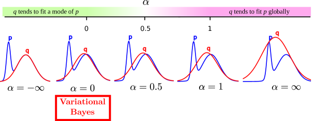
which includes a parameter $\alpha\in\mathbb{R}$ that controls the properties of the optimal $q$. Figure 1 illustrates these properties for the one-dimensional case. When $\alpha\geq 1$, $q$ tends to cover the whole posterior distribution $p$. When $\alpha\leq 0$, $q$ tends to fit a local mode in $p$. The value $\alpha=0.5$ is expected to achieve a balance between these two tendencies. Importantly, when $\alpha\rightarrow 0$, the solution obtained is the same as with variational Bayes (VB) (Wainwright & Jordan, 2008).

The direct minimization of (6) is infeasible in practice for arbitrary $\alpha$. Instead, we follow Hernández-Lobato et al. (2016) and optimize an energy function whose minimizer corresponds to a local minimization of $\alpha$-divergences, with one $\alpha$-divergence for each of the $N$ likelihood factors in (1). Since $q$ is Gaussian and the priors $p(\mathcal{W})$ and $p(\mathbf{z})$ are also Gaussian, we represent $q$ as

$$q(\mathcal{W},\mathbf{z})\propto\left[\prod_{n=1}^{N}f(\mathcal{W})f_{n}(z_{n})\right]p(\mathcal{W})p(\mathbf{z})\,,$$ (7)

where $f(\mathcal{W})$ is a Gaussian factor that approximates the geometric mean of the $N$ likelihood factors in (1) as a function of $\mathcal{W}$. Each $f_{n}(z_{n})$ is also a Gaussian factor that approximates the $n$-th likelihood factor in (1) as a function of $z_{n}$. We adjust $f(\mathcal{W})$ and the $f_{n}(z_{n})$ by minimizing local $\alpha$-divergences. In particular, we minimize the energy function

$$E_{\alpha}(q)=-\log Z_{q}-\frac{1}{\alpha}\sum_{n=1}^{N}\log\mathbf{E}_{\mathcal{W},z_{n}\sim\,q}\left[\left(\frac{p(\mathbf{y}_{n}\,|\,\mathcal{W},\mathbf{x}_{n},z_{n},\bm{\Sigma})}{f(\mathcal{W})f_{n}(z_{n})}\right)^{\alpha}\right]\,,$$ (8)

(Hernández-Lobato et al., 2016), where $f(\mathcal{W})$ and $f_{n}(z_{n})$ are in exponential Gaussian form and parameterized in terms of the parameters of $q$ and the priors $p(\mathcal{W})$ and $p(z_{n})$, that is,

$$f(\mathcal{W})= \exp\left\{\sum_{l=1}^{L}\!\sum_{i=1}^{V_{l}}\!\sum_{j=1}^{V_{l\!-\!1}\!+\!1}\frac{1}{N}\left(\frac{\lambda v^{w}_{i,j,l}}{\lambda-v^{w}_{i,j,l}}w_{i,j,l}^{2}+\frac{m^{w}_{i,j,l}}{v^{w}_{i,j,l}}w_{i,j,l}\right)\right\}\propto\left[\frac{q(\mathcal{W})}{p(\mathcal{W})}\right]^{\frac{1}{N}}\,,$$ (9)

$$f_{n}(z_{n})= \exp\left\{\frac{\gamma v^{z}_{n}}{\gamma-v^{z}_{n}}z_{n}^{2}+\frac{m^{z}_{n}}{v^{z}_{n}}z_{n}\right\}\propto\frac{q(z_{n})}{p(z_{n})}\,,$$ (10)

and $\log Z_{q}$ is the logarithm of the normalization constant of the exponential Gaussian form of $q$:

$$\log Z_{q}=\sum_{l=1}^{L}\!\sum_{i=1}^{V_{l}}\!\sum_{j=1}^{V_{l\!-\!1}\!+\!1}\left[\frac{1}{2}\log\left(2\pi v^{w}_{i,j,l}\right)+\frac{\left(m^{w}_{i,j,l}\right)^{2}}{v^{w}_{i,j,l}}\right]+\sum_{n=1}^{N}\left[\frac{1}{2}\log\left(2\pi v^{z}_{n}\right)+\frac{\left(m^{z}_{n}\right)^{2}}{v^{z}_{n}}\right]\,.$$ (11)

The scalable optimization of (8) is done in practice by using stochastic gradient descent. For this, we subsample the sums for $n=1,\ldots,N$ in (8) and (11) using mini-batches and approximate the expectations over $q$ in (8) with an average over $K$ samples drawn from $q$. We can then use the reparametrization trick (Kingma et al., 2015) to obtain gradients from the resulting stochastic approximator to (8). The hyper-parameters $\bm{\Sigma}$, $\lambda$ and $\gamma$ can also be tuned by minimizing (8). In practice we only tune $\bm{\Sigma}$ and keep $\lambda=1$ and $\gamma=d$. The latter means that the prior scale of each $z_{n}$ grows with the data dimensionality. This guarantees that, a priori, the effect of each $z_{n}$ in the neural network’s output does not diminish when more and more features are available.

Minimizing (8) when $\alpha\rightarrow 0$ is equivalent to running the method VB (Hernández-Lobato et al., 2016), which has recently been used to train Bayesian neural networks in reinforcement learning problems (Blundell et al., 2015; Houthooft et al., 2016; Gal et al., 2016). However, we propose to minimize (8) using $\alpha=0.5$, which often results in better test log-likelihood values.

We have also observed $\alpha=0.5$ to be more robust than VB when $q(\mathbf{z})$ is not fully optimized. In particular, $\alpha=0.5$ can still capture complex stochastic patterns even when we do not learn $q(\mathbf{z})$ and instead keep it fixed to the prior $p(\mathbf{z})$. By contrast, VB fails completely in this case (see Appendix A).

3 Policy search using BNNs with stochastic inputs

We now describe a gradient-based policy search algorithm that uses the BNNs with stochastic disturbances from the previous section. The motivation for our approach lies in its applicability to industrial systems: we wish to estimate a policy in parametric form, using only an available batch of state transitions obtained from an already-running system. We assume that the true dynamics present stochastic patterns that arise due to some unobserved process affecting the system in complex ways.

Model-based policy search methods include two key parts (Deisenroth et al., 2013). The first part consists in learning a dynamics model from data in the form of state transitions $(\mathbf{s}_{t},\mathbf{a}_{t},\mathbf{s}_{t+1})$, where $\mathbf{s}_{t}$ denotes the current state, $\mathbf{a}_{t}$ is the action applied and $\mathbf{s}_{t+1}$ is the resulting state. The second part consists in learning the parameters $\mathcal{W}_{\pi}$ of a deterministic policy function $\pi$ that returns the optimal action $\mathbf{a}_{t}=\pi(\mathbf{s}_{t};\mathcal{W}_{\pi})$ as function of the current state $\mathbf{s}_{t}$. The policy function can be a neural network with deterministic weights given by $\mathcal{W}_{\pi}$.

The first part in the aforementioned procedure is a standard regression task, which we solve by using the modeling approach from the previous section. We assume the dynamics to be stochastic with the following true transition model:

$$\mathbf{s}_{t}=f_{\text{true}}(\mathbf{s}_{t-1},\mathbf{a}_{t-1},z_{t};\mathcal{W}_{\text{true}})\,,\quad z_{t}\sim\mathcal{N}(0,\gamma)\,.$$ (12)

where the input disturbances $z_{t}\sim\mathcal{N}(0,\gamma)$ account for the stochasticity in the dynamics. When the Markov state $\mathbf{s}_{t}$ is hidden and we are given only observations $\mathbf{o}_{t}$ , we can use the time embedding theorem using a suitable window of length $n$ and approximate:

$$\hat{\mathbf{s}}(t)=[\mathbf{o}_{t-n},\cdots,\mathbf{o}_{t}]\,.$$ (13)

The transition model in equation 12 specifies a probability distribution $p(\mathbf{s}_{t}|\mathbf{s}_{t-1},\mathbf{a}_{t-1})$ that we approximate using a BNN with stochastic inputs:

$$p(\mathbf{s}_{t}|\mathbf{s}_{t-1},\mathbf{a}_{t-1})\approx\int\mathcal{N}(\mathbf{s}_{t}|f(\mathbf{s}_{t-1},\mathbf{a}_{t-1},z_{t};\mathcal{W}),\bm{\Sigma})q(\mathcal{W})\mathcal{N}(z_{t}|0,\gamma)\,d\mathcal{W}\,dz_{t}\,,$$ (14)

where the feature vectors in our BNN are now $\mathbf{s}_{t-1}$ and $\mathbf{a}_{t-1}$ and the targets are given by $\mathbf{s}_{t}$. In this expression, the integration with respect to $\mathcal{W}$ accounts for stochasticity arising from lack of knowledge of the model parameters, while the integration with respect to $z_{t}$ accounts for stochasticity arising from unobserved processes that cannot be modeled. In practice, these integrals are approximated by an average over samples of $z_{t}\sim\mathcal{N}(0,\gamma)$ and $\mathcal{W}\sim q$.

In the second part of our model-based policy search algorithm, we optimize the parameters $\mathcal{W}_{\pi}$ of a policy that minimizes the sum of expected cost over a finite horizon $T$ with respect to our belief $q(\mathcal{W})$. This expected cost is obtained by averaging over multiple virtual roll-outs. For each roll-out we sample $\mathcal{W}_{i}\sim q$ and then simulate state trajectories using the model $\mathbf{s}_{t+1}=f(\mathbf{s}_{t},\mathbf{a}_{t},z_{t};\mathcal{W}_{i})+\bm{\epsilon}_{t+1}$ with policy $\mathbf{a}_{t}=\pi(\mathbf{s}_{t};\mathcal{W}_{\pi})$, input noise $z_{t}\sim\mathcal{N}(0,\gamma)$ and additive noise $\bm{\epsilon}_{t+1}\sim\mathcal{N}(\bm{0},\bm{\Sigma})$. This procedure allows us to obtain estimates of the policy’s expected cost for any particular cost function. If model, policy and cost function are differentiable, we are then able to tune $\mathcal{W}_{\pi}$ by stochastic gradient descent over the roll-out average.

1:Input: $\mathcal{D}=\{\mathbf{s}_{n},a_{n},\bm{\Delta}_{n}\}$ for $n\in 1..N$ 2:Fit $q(\mathcal{W})$ and $\bm{\Sigma}$ by optimizing (8). 3:function unfold($\mathbf{s}_{0}$) 4:     $\textit{sample}\{\mathcal{W}^{1},..,\mathcal{W}^{K}\}\textit{ from }q(\mathcal{W})$ 5:     $C\leftarrow 0$ 6:     for $k=1:K$ do 7:         for $t=0:T$ do 8:              $z_{t+1}^{k}\sim\mathcal{N}(0,\gamma)$ 9:              $\bm{\Delta}_{t}\leftarrow f(\mathbf{s}_{t},\pi(\mathbf{s}_{t};\mathcal{W}_{\pi}),z_{t+1}^{k};\mathcal{W}^{k})$ 10:              $\bm{\epsilon}_{t+1}^{k}\sim\mathcal{N}(\mathbf{0},\bm{\Sigma})$ 11:              $\mathbf{s}_{t+1}\leftarrow\mathbf{s}_{t}+\bm{\Delta}_{t}+\bm{\epsilon}_{t+1}^{k}$ 12:              $C\leftarrow C+c(\mathbf{s}_{t+1})$                13:     return $C/K$ 14:Fit $\mathcal{W}_{\pi}$ by optimizing $\frac{1}{N}\sum_{n=1}^{N}$ unfold($\mathbf{s}_{n}$) Algorithm 1 Model-based policy search using
Bayesian neural networks with stochastic inputs.

Figure 2: Predictive distribution of $y_{t}$ given by different methods in four different scenarios. Ground truth (red) is obtained by sampling from the real dynamics.

Given a cost function $c(\mathbf{s}_{t})$, the objective to be optimized by our policy search algorithm is

$$\textstyle J(\mathcal{W}_{\pi}) =\textstyle\mathbf{E}\left[\sum_{t=1}^{T}c(\mathbf{s}_{t})\right]\,.$$ (15)

We approximate (15) by using (14), replacing $\mathbf{a}_{t}$ with $\pi(\mathbf{s}_{t};\mathcal{W}_{\pi})$ and using sampling to approximate the expectations:

$$J(\mathcal{W}_{\pi})= \int\left[\sum_{t=1}^{T}c(\mathbf{s}_{t})\right]\left[\prod_{t=1}^{T}\int\mathcal{N}(\mathbf{s}_{t}|f(\mathbf{s}_{t-1},\pi(\mathbf{s}_{t-1};\mathcal{W}_{\pi}),z_{t};\mathcal{W}),\bm{\Sigma})q(\mathcal{W})\mathcal{N}(z_{t}|0,\gamma)\,d\mathcal{W}\,dz_{t}\right]$$

$$p(\mathbf{s}_{0})d\mathbf{s}_{0}\cdots d\mathbf{s}_{T}$$

$$= \int\left[\sum_{t=1}^{T}c(\mathbf{s}_{t}^{\mathcal{W},\{z_{1},\ldots,z_{t}\},\{\bm{\epsilon}_{1},\ldots,\bm{\epsilon}_{t}\},\mathcal{W}_{\pi}})\right]q(\mathcal{W})d\mathcal{W}\left[\prod_{t=1}^{T}\mathcal{N}(\bm{\epsilon}_{t}|\mathbf{0},\bm{\Sigma})\mathcal{N}(z_{t}|0,\gamma)d\bm{\epsilon}_{t}dz_{t}\right]p(\mathbf{s}_{0})\,d\mathbf{s}_{0}$$

$$\approx \frac{1}{K}\sum_{k=1}^{K}\left[\sum_{t=1}^{T}c(\mathbf{s}_{t}^{\mathcal{W}^{k},\{z_{1}^{k},\ldots,z_{t}^{k}\},\{\bm{\epsilon}_{1}^{k},\ldots,\bm{\epsilon}_{t}^{k}\},\mathcal{W}_{\pi}})\right]\,.$$ (16)

The first line in (16) is obtained by using the assumption that the dynamics are Markovian with respect to the current state and the current action and by replacing $p(\mathbf{s}_{t}|\mathbf{s}_{t-1},\mathbf{a}_{t-1})$ with the right-hand side of (14). In the second line, $\mathbf{s}_{t}^{\mathcal{W},\{z_{1},\ldots,z_{t}\},\{\bm{\epsilon}_{1},\ldots,\bm{\epsilon}_{t}\},\mathcal{W}_{\pi}}$ is the state that is obtained at time $t$ in a roll-out generated by using a policy with parameters $\mathcal{W}_{\pi}$, a transition function parameterized by $\mathcal{W}$ and input noise $z_{1},\ldots,z_{t}$, with additive noise values $\bm{\epsilon}_{1},\ldots,\bm{\epsilon}_{t}$. In the last line we have approximated the integration with respect to $\mathcal{W},z_{1},\ldots,z_{T}$, $\bm{\epsilon}_{1},\ldots,\bm{\epsilon}_{T}$ and $\mathbf{s}_{0}$ by averaging over $K$ samples of these variables. To sample $\mathbf{s}_{0}$, we draw this variable uniformly from the available transitions $(\mathbf{s}_{t},\mathbf{a}_{t},\mathbf{s}_{t+1})$.

The expected cost (15) can then be optimized by stochastic gradient descent using the gradients of the Monte Carlo approximation given by the last line of (16). Algorithm 1 computes this Monte Carlo approximation. The gradients can then be obtained using automatic differentiation tools such as Theano (Theano Development Team, ). Note that Algorithm 1 uses the BNNs to make predictions for the change in the state $\Delta_{t}=\mathbf{s}_{t+1}-\mathbf{s}_{t}$ instead of for the next state $\mathbf{s}_{t+1}$ since this approach often performs better in practice (Deisenroth & Rasmussen, 2011).

4 Experiments

We now evaluate the performance of our algorithm for policy search in different benchmark problems. These problems are chosen based on two reasons. First, they contain complex stochastic dynamics and second, they represent real-world applications common in industrial settings. A theano implementation of algorithm 1 is available online. See the appendix B for a short introduction to all methods we compare to and appendix C for the hyper-parameters used.

4.1 Wet-Chicken benchmark

Figure 3: Visualization of three policies in state space. Waterfall is indicated by top black bar. Left: policy $\pi_{VB}$ obtained with a BNN trained with VB. Avg. reward is $-2.53$. Middle: policy $\pi_{\alpha=0.5}$ obtained with a BNN trained with $\alpha=0.5$. Avg. reward is $-2.31$. Right: policy $\pi_{GP}$ obtained by using a Gaussian process model. Avg. reward is $-2.94$. Color and arrow indicate direction of paddling of policy when in state $\mathbf{s}_{t}$, arrow length indicates action magnitude. Best viewed in color.

The Wet-Chicken benchmark (Tresp, 1994) is a challenging problem for model-based policy search that presents both bi-modal and heteroskedastic transition dynamics. We use the two-dimensional version of the problem (Hans & Udluft, 2009) and extend it to the continuous case.

Dataset	MLP		VB		$\boldsymbol{\alpha{=}0.5}$		$\boldsymbol{\alpha{=}1.0}$		GP		PSO-P
Wetchicken	-2.71$\pm$	0.09	-2.67$\pm$	0.10	-2.37$\pm$	0.01	-2.42$\pm$	0.01	-3.05$\pm$	0.06	-2.34
Turbine	-0.65$\pm$	0.14	-0.45$\pm$	0.02	-0.41$\pm$	0.03	-0.55$\pm$	0.08	-0.64$\pm$	0.18	NA
Industrial	-183.5$\pm$	4.1	-180.2$\pm$	0.6	-174.2$\pm$	1.1	-171.1$\pm$	2.1	-285.2$\pm$	20.5	-145.5
Avg. Rank	3.6$\pm$	0.3	3.1$\pm$	0.2	1.5$\pm$	0.2	2.3$\pm$	0.3	4.5$\pm$	0.3

Table 1: Policy performances over different benchmarks. Printed are average values over $5$ runs with respective standard errors. Bottom row is the average rank over all $5\times 3$ runs.

Dataset	MLP		VB		$\boldsymbol{\alpha{=}0.5}$		$\boldsymbol{\alpha{=}1.0}$		GP
MSE
WetChicken	1.289$\pm$	0.013	1.347$\pm$	0.015	1.347$\pm$	0.008	1.359$\pm$	0.017	1.359$\pm$	0.017
Turbine	0.16$\pm$	0.001	0.21$\pm$	0.003	0.192$\pm$	0.002	0.237$\pm$	0.004	0.492$\pm$	0.026
Industrial	0.0186$\pm$	0.0052	0.0182$\pm$	0.0052	0.017$\pm$	0.0046	0.0171$\pm$	0.0047	0.0233$\pm$	0.0049
Avg. Rank	2.0$\pm$	0.34	3.1$\pm$	0.24	2.4$\pm$	0.23	2.9$\pm$	0.36	4.6$\pm$	0.23
Log-Likelihood
WetChicken	-1.755$\pm$	0.003	-1.140$\pm$	0.033	-1.057$\pm$	0.014	-1.070$\pm$	0.011	-1.722$\pm$	0.011
Turbine	-0.868$\pm$	0.007	-0.775$\pm$	0.004	-0.746$\pm$	0.013	-0.774$\pm$	0.015	-2.663$\pm$	0.131
Industrial	0.767$\pm$	0.047	1.132$\pm$	0.064	1.328$\pm$	0.108	1.326$\pm$	0.098	0.724$\pm$	0.04
Avg. Rank	4.3$\pm$	0.12	2.6$\pm$	0.16	1.3$\pm$	0.15	2.1$\pm$	0.18	4.7$\pm$	0.12

Table 2: Model test error and test log-likelihood for different benchmarks. Printed are average values over 5 runs with respective standard errors. Bottom row is the average rank over all $5\times 3$ runs.

In this problem, a canoeist is paddling on a two-dimensional river. The canoeist’s position at time $t$ is $(x_{t},y_{t})$. The river has width $w=5$ and length $l=5$ with a waterfall at the end, that is, at $y_{t}=l$. The canoeist wants to move as close to the waterfall as possible because at time $t$ he gets reward $r_{t}=-(l-y_{t})$. However, going beyond the waterfall boundary makes the canoeist fall down, having to start back again at the origin $(0,0)$. At time $t$ the canoeist can choose an action $(a_{t,x},a_{t,y})\in[-1,1]^{2}$ that represents the direction and magnitude of his paddling. The river dynamics have stochastic turbulences $s_{t}$ and drift $v_{t}$ that depend on the canoeist’s position on the $x$ axis. The larger $x_{t}$, the larger the drift and the smaller $x_{t}$, the larger the turbulences. The underlying dynamics are given by the following system of equations. The drift and the turbulence magnitude are given by $v_{t}=3x_{t}w^{-1}$ and $s_{t}=3.5-v_{t}$, respectively. The new location $(x_{t+1},y_{t+1})$ is given by the current location $(x_{t},y_{t})$ and current action $(a_{t,x},a_{t,y})$ using

$$x_{t+1} =\begin{cases}0&\text{if }\quad x_{t}+a_{t,x}<0\\ 0&\text{if }\quad\hat{y}_{t+1}>l\\ w&\text{if }\quad x_{t}+a_{t,x}>w\\ x_{t}+a_{t,x}&\text{otherwise}\end{cases}\,, y_{t+1} =\begin{cases}0&\text{if }\quad\hat{y}_{t+1}<0\\ 0&\text{if }\quad\hat{y}_{t+1}>l\\ \hat{y}_{t+1}&\text{otherwise}\end{cases}\,,$$ (17)

where $\hat{y}_{t+1}=y_{t}+(a_{t,y}-1)+v_{t}+s_{t}\tau_{t}$ and $\tau_{t}\sim\text{Unif}([-1,1])$ is a random variable that represents the current turbulence. These dynamics result in rich transition distributions depending on the position as illustrated by the plots in Figure 2. As the canoeist moves closer to the waterfall, the distribution for the next state becomes increasingly bi-modal (see Figure 2) because when he is close to the waterfall, the change in the current location can be large if the canoeist falls down the waterfall and starts again at $(0,0)$. The distribution may also be truncated uniform for states close to the borders (see Figure 2). Furthermore the system has heteroskedastic noise, the smaller the value of $x_{t}$ the higher the noise variance (compare Figure 2 with 2). Because of these properties, the Wet-Chicken problem is especially difficult for model-based reinforcement learning methods. To our knowledge it has only been solved using model-free approaches after a discretization of the state and action sets (Hans & Udluft, 2009). For model training we use a batch 2500 random state transitions.

The predictive distributions of different models for $y_{t+1}$ are shown in Figure 2 for specific choices of $(x_{t},y_{t})$ and $(a_{x,t},a_{y,t})$. These plots show that BNNs with $\alpha=0.5$ are very close to the ground-truth. While it is expected that Gaussian processes fail to model multi-modalities in Figure 2, the FTIC approximation allows them to model the heteroskedasticity to an extent. VB captures the stochastic patterns on a global level, but often under or over-estimates the true probability density in specific regions. The test-loglikelihood and test MSE in $y$-dimension are reported in Table 2 for all methods. (the transitions for $x$ are deterministic given $y$).

After fitting the models, we train policies using Algorithm 1 with a horizon of size $T=5$. Table 1 shows the average reward obtained by each method. BNNs with $\alpha=0.5$ perform best and produce policies that are very close to the optimal upper bound, as indicated by the performance of the particle swarm optimization policy (PSO-P). In this problem VB seems to lack robustness and has much larger empirical variance across experiment repetitions than $\alpha=0.5$ or $\alpha=1.0$.

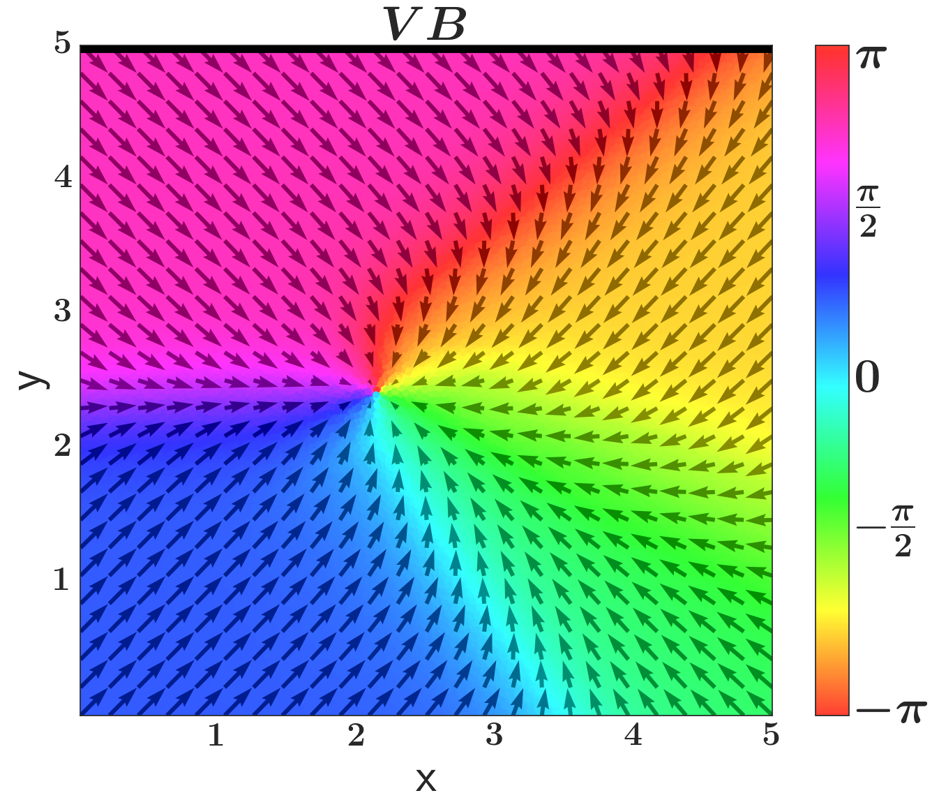
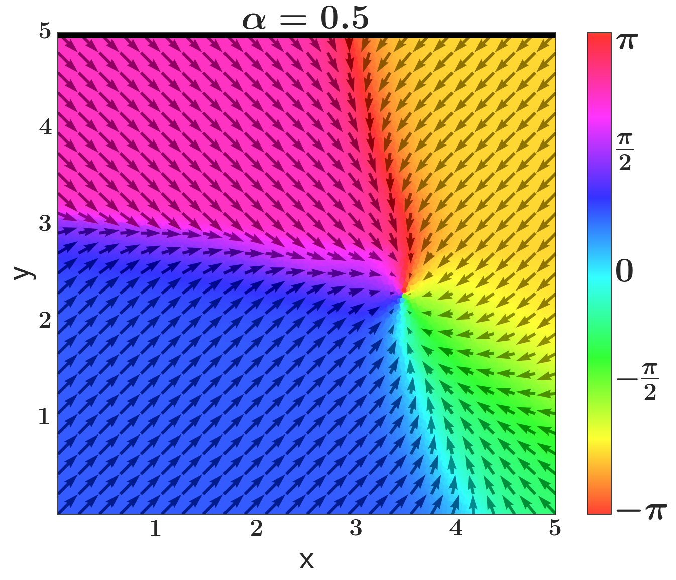
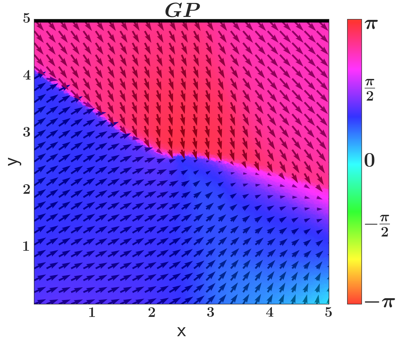
Figure 3 shows three example policies, $\pi_{\text{VB}}$ ,$\pi_{\alpha=0.5}$ and $\pi_{\text{GP}}$ (Figure 3,3 and 3, respectively). The policies obtained by BNNs with random inputs (VB and $\alpha=0.5$) show a richer selection of actions. The biggest differences are in the middle-right regions of the plots, where the drift towards the waterfall is large and the bi-modal transition for $y$ (missed by the GP) is more important.

Figure 4: Roll-outs of algorithm 1 for two starting states $\mathbf{s}_{0}$ (top/bottom) using different types of BNNs (left to right) with $K=75$ samples for $T=75$ steps. Action sequence $A_{0},\cdots,A_{T=75}$ given by dataset for each $\mathbf{s}_{0}$. From left to right: model trained using VB,$\alpha=0.5$ and $\alpha=1.0$ respectively. Red: trajectory observed in dataset, blue: sample average, light blue: individual samples.

4.2 Industrial applications

We now present results on two industrial cases. First, we focus on data generated by a real gas turbine and second, we consider a recently introduced simulator called the "industrial benchmark", with code publicly available (Hein et al., 2016b). According to the authors: "The "industrial benchmark" aims at being realistic in the sense, that it includes a variety of aspects that we found to be vital in industrial applications."

4.2.1 Gas turbine data

For the experiment with gas turbine data we simulate a task with partial observability. To that end we use 40,000 observations of a 30 dimensional time-series of sensor recordings from a real gas turbine. We are also given a cost function that evaluates the performance of the current state of the turbine. The features in the time-series are grouped into three different sets: a set of environmental variables $E_{t}$ (e.g. temperature and measurements from sensors in the turbine) that cannot be influenced by the agent, a set of variables relevant for the cost function $N_{t}$ (e.g. the turbines current pollutant emission) and a set of steering variables $A_{t}$ that can be manipulated to control the turbine.

We first train a world model as a reflection of the real turbine dynamics. To that end we define the world model’s transitions for $N_{t}$ to have the functional form $N_{t}=f(E_{t-5},..,E_{t},A_{t-5},..A_{t})$. The world model assumes constant transitions for the environmental variables: $E_{t+1}=E_{t}$. To make fair comparisons, our world model is given by a non-Bayesian neural network with deterministic weights and with additive Gaussian output noise.

We then use the world model to generate an artificial batch of data for training the different methods. The inputs in this batch are still the same as in the original turbine data, but the outputs are now sampled from the world model. After generating the artificial data, we only keep a small subset of the original inputs to the world model. The aim of this experiment is to learn policies that are robust to noise in the dynamics. This noise would originate from latent factors that cannot be controlled, such as the missing features that were originally used to generate the outputs by the world model but which are no longer available. After training the models for the dynamics, we use algorithm 1 for policy optimization. The resulting policies are then finally evaluated in the world model.

Tables 2 and 1 show the respective model and policy performances for each method. The experiment was repeated $5$ times and we report average results. We observe that $\alpha=0.5$ performs best in this scenario, having the highest test log-likelihood and best policy performance.

4.2.2 Industrial benchmark

In this benchmark the hidden Markov state space $\mathbf{s}_{t}$ consists of $27$ variables, whereas the observable state $\mathbf{o}_{t}$ is only 5 dimensional. This observable state consists of 3 adjustable steering variables $A_{t}$: the velocity $v(t)$, the gain $g(t)$ and the shift $s(t)$. We also observe the fatigue $f(t)$ and consumption $c(t)$ that together form the reward signal $R(t)=-(3f(t)+c(t))$. Also visible is the setpoint $S$, a constant hyper-parameter of the benchmark that indicates the complexity of the dynamics.

For each setpoint $S\in\{10,20,\cdots,100\}$ we generate $7$ trajectories of length $1000$ using random exploration. This batch with $70,000$ state transitions forms the training set. We use $30,000$ state transitions, consisting of $3$ trajectories for each setpoint, as test set.

For data preprocessing, in addition to the standard normalization process, we apply a log transformation to the reward variable. Because the reward is bounded in the interval $[0,R_{max}]$, we use a logit transformation to map this interval into the real line. We define the functional form for the dynamics as $R_{t}=f(A_{t-15},\cdots,A_{t},R_{t-15},\cdots,R_{t-1})$.

The test errors and log-likelihood are given in Table 2. We see that BNNs with $\alpha=0.5$ and $\alpha=1.0$ perform best here, whereas Gaussian processes or the MLP obtain rather poor results.

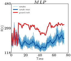
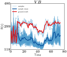
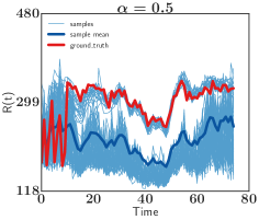
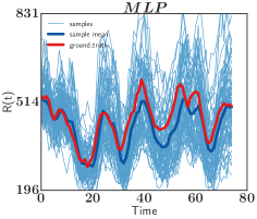
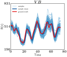
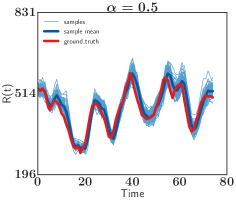
Each row in Figure 4 visualizes long term predictions of the MLP and BNNs trained with VB and $\alpha=0.5$ in two specific cases. In the top row we see that while all three methods produce wrong predictions in expectation (compare dark blue curve to red curve). However, BNNs trained with $VB$ and with $\alpha=0.5$ exhibit a bi-modal distribution of predicted trajectories, with one mode following the ground-truth very closely. By contrast, the MLP misses the upper mode completely. The bottom row shows that the VB and $\alpha=0.5$ also produce more tight confident bands in other settings.

Next, we learn policies using the trained models. Here we use a relatively long horizon of $T=75$ steps. Table 1 shows average rewards obtained when applying the policies to the real dynamics. Because both benchmark and models have an autoregressive component, we do an initial warm-up phase using random exploration before we apply the policies to the system and start to measure rewards.

We observe that GPs perform very poorly in this benchmark. We believe the reason for this is the long search horizon, which makes the uncertainties in the predictive distributions of the GPs become very large. Tighter confidence bands, as illustrated in Figure 4 seem to be key for learning good policies. Overall, $\alpha=1.0$ performs best with $\alpha=0.5$ being very close.

5 Related work

There has been relatively little attention to using Bayesian neural networks for reinforcement learning. In Blundell et al. (2015) a Thompson sampling approach is used for a contextual bandits problem; the focus is tackling the exploration-exploitation trade-off, while the work in Watter et al. (2015) combines variational auto-encoder with stochastic optimal control for visual data. Compared to our approach the first of these contributions focusses on the exploration/exploitation dilemma, while the second one uses a stochastic optimal control approach to solve the learning problem. By contrast, our work seeks to find an optimal parameterized policy.

Policy gradient techniques are a prominent class of policy search algorithms (Peters & Schaal, 2008). While model-based approaches were often used in discrete spaces (Wang & Dietterich, 2003), model-free approaches tended to be more popular in continuous spaces (e.g. Peters & Schaal (2006)).

Our work can be seen as a Monte-Carlo model-based policy gradient technique in continuous stochastic systems. Similar work was done using Gaussian processes (Deisenroth & Rasmussen, 2011) and with recurrent neural networks (Schaefer et al., 2007) . The Gaussian process approach, while restricted to a Gaussian state distribution, allows propagating beliefs over the roll-out procedure. More recently Gu et al. (2016) augment a model-free learning procedure with data generated from model-based roll-outs.

6 Conclusion and future work

We have extended the standard Bayesian neural network (BNN) model with the addition of a random input noise source $z$. This enables principled Bayesian inference over complex stochastic functions. We have shown that our BNNs with random inputs can be trained with high accuracy by minimizing $\alpha$-divergences, with $\alpha=0.5$, which often produces better results than variational Bayes. We have also presented an algorithm that uses random roll-outs and stochastic optimization for learning a parameterized policy in a batch scenario. This algorithm particular suited for industry domains.

Our BNNs with random inputs have allowed us to solve a challenging benchmark problem where model-based approaches usually fail. They have also shown promising results on industry benchmarks including real-world data from a gas turbine. In particular, our experiments indicate that a BNN trained with $\alpha=0.5$ as divergence measure in conjunction with the presented algorithm for policy optimization is a powerful black-box tool for policy search.

As future work we will consider safety and exploration. For safety, we believe having uncertainty over the underlaying stochastic functions will allows us to optimize policies by focusing on worst case results instead of on average performance. For exploration, having uncertainty on the stochastic functions will be useful for efficient data collection.

Acknowledgements

José Miguel Hernández-Lobato acknowledges support from the Rafael del Pino Foundation. The authors would like to thank Ryan P. Adams, Hans-Georg Zimmermann, Matthew J. Johnson, David Duvenaud and Justin Bayer for helpful discussions.

Appendix A Robustness of $\alpha=0.5$ and $\alpha=1.0$ when $q(\mathbf{z})$ is not learned

We evaluate the accuracy of the predictive distributions generated by BNNs with stochastic inputs trained by minimizing (8) for different BNNs parameterized by $\alpha$ in two simple regression problems. The first one is characterized by a bimodal predictive distribution. The second is characterized by a heteroskedastic predictive distribution. In the latter case the magnitude of the noise in the targets changes as a function of the input features.

In the first problem $x\in[-2,2]$ and $y$ is obtained as $y=10\sin(x)+\epsilon$ with probability $0.5$ and $y=10\cos(x)+\epsilon$, otherwise, where $\epsilon\sim\mathcal{N}(0,1)$ and $\epsilon$ is independent of $x$. The plot in the top of the 1st column in Figure 5 shows a training dataset obtained by sampling 2500 values of $x$ uniformly at random. The plot clearly shows that the distribution of $y$ for a particular $x$ is bimodal. In the second problem $x\in[-4,4]$ and $y$ is obtained as $y=7\sin(x)+3|\cos(x/2)|\epsilon$. The plot in the bottom of the 1st column in Figure 5 shows a training dataset obtained with 1000 values of $x$ uniformly at random. The plot clearly shows that the distribution of $y$ is heteroskedastic, with a noise variance that is a function of $x$.

We evaluated the predictive performance obtained by minimizing (8) using $\alpha=0.5$ and $\alpha=1.0$ and also by running VB. However, we do not learn $q(\mathbf{z})$ and keeping it instead fixed to the prior $p(\mathbf{z})$.

We fitted a neural network with 2 hidden layers and 50 hidden units per layer using Adam with its default parameter values, with a learning rate of 0.01 in the first problem and 0.002 in the second problem. We used mini-batches of size 250 and 1000 training epochs. To approximate the expectations in 8, we draw $K=50$ samples from $q$.

Figure 5: Ground truth and predictive distributions for two toy problems introduced in main text. Top: bi-modal prediction problem, Bottom: heteroskedastic prediction problem. Left column: Training data (blue points) and ground truth functions (red). Columns 2-4: predictions generated with VB, $\alpha=0.5$ and $\alpha=1.0$, respectively.

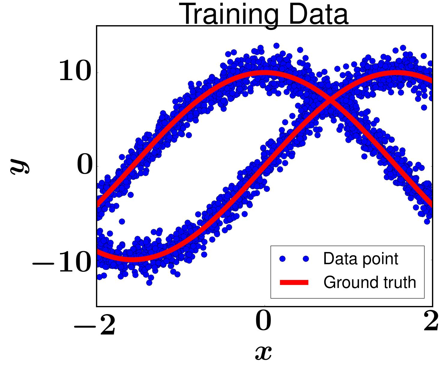
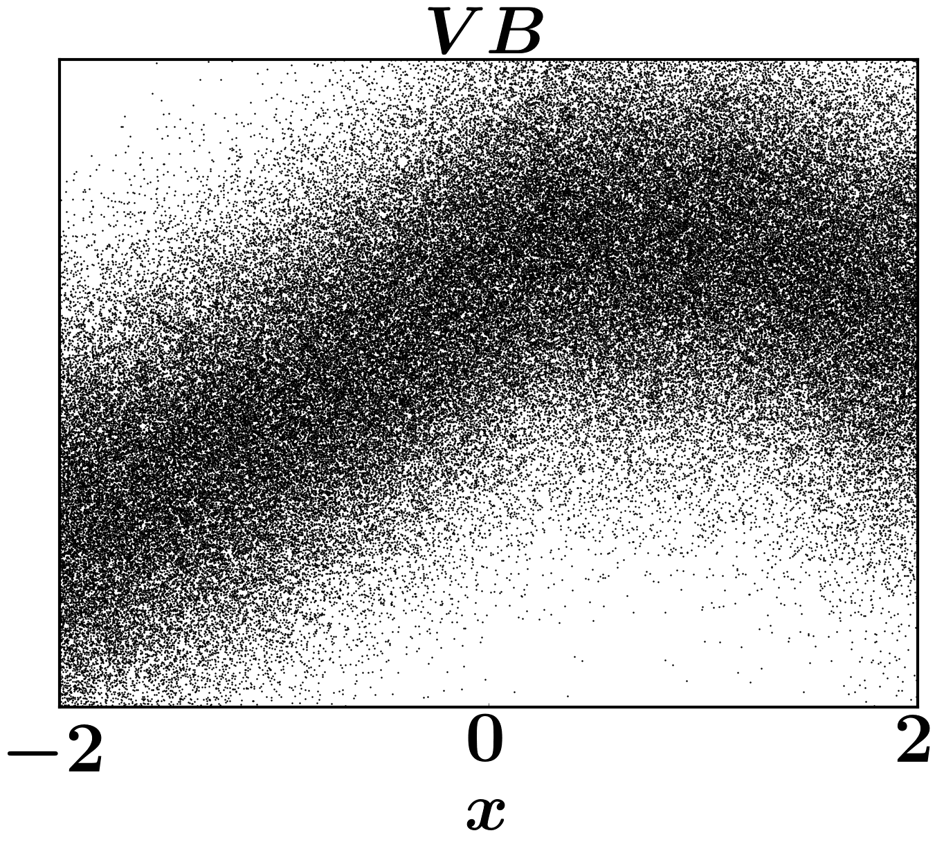
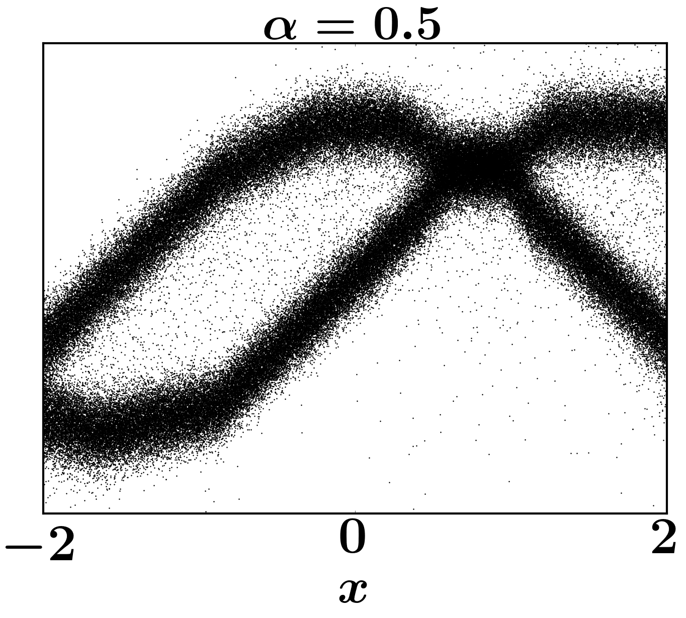
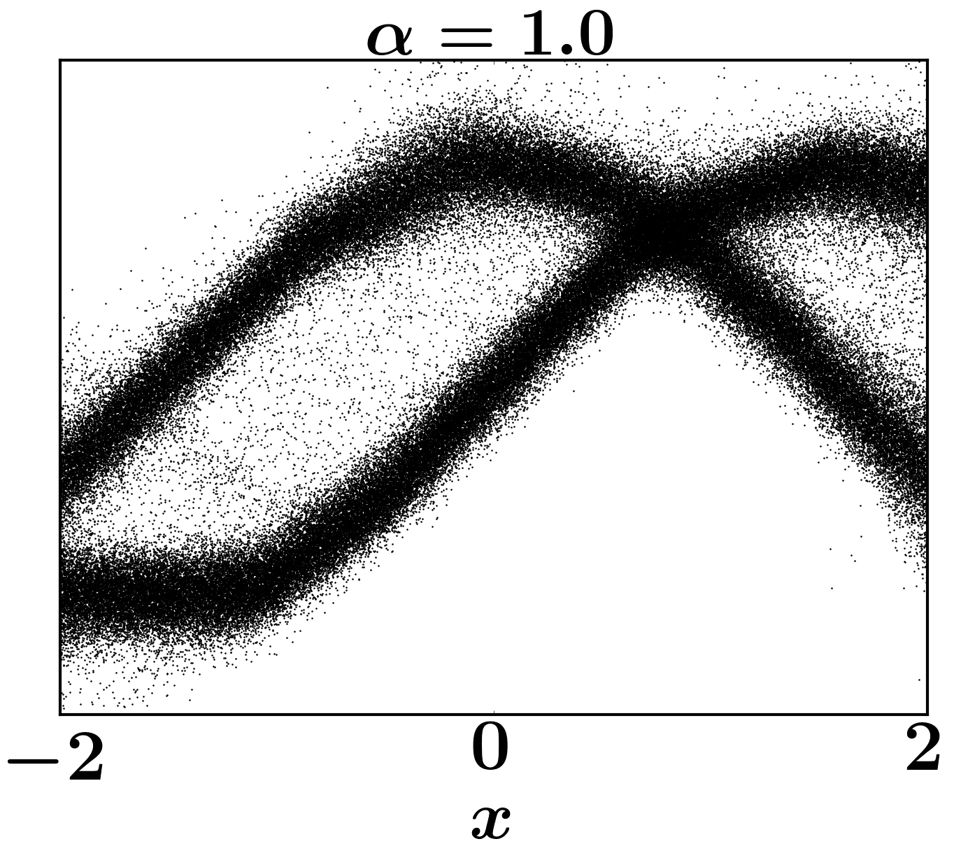
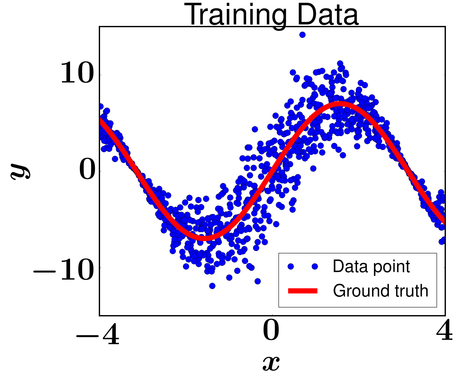
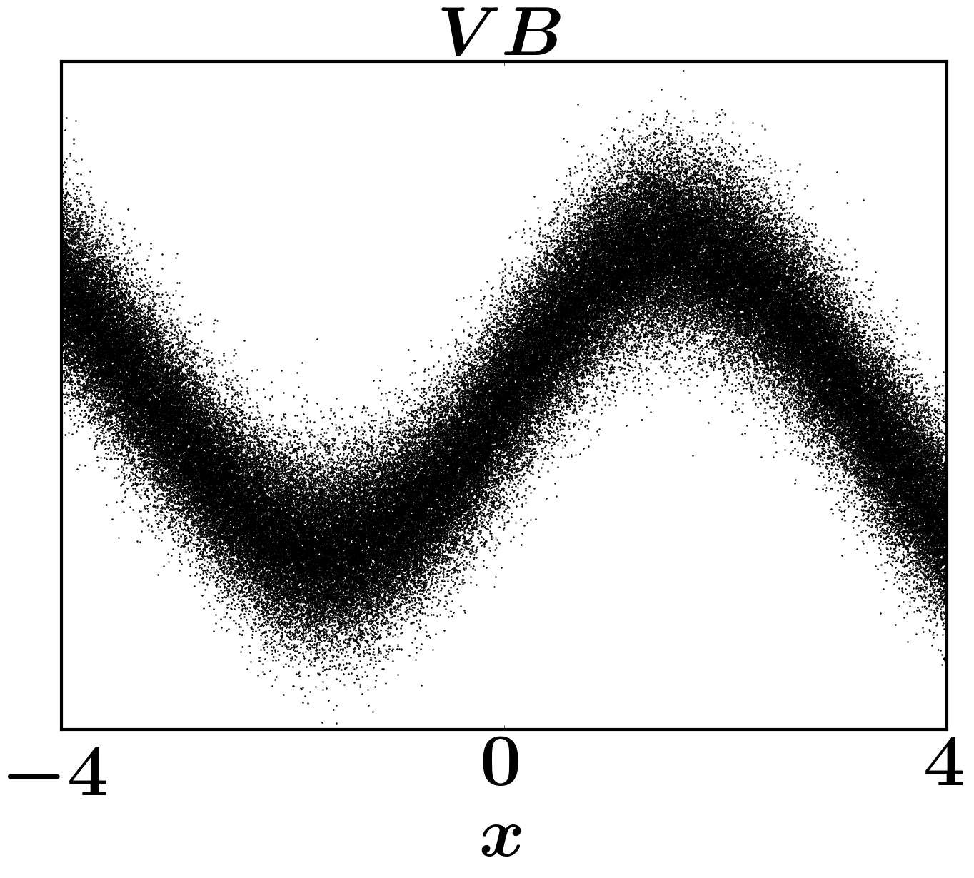
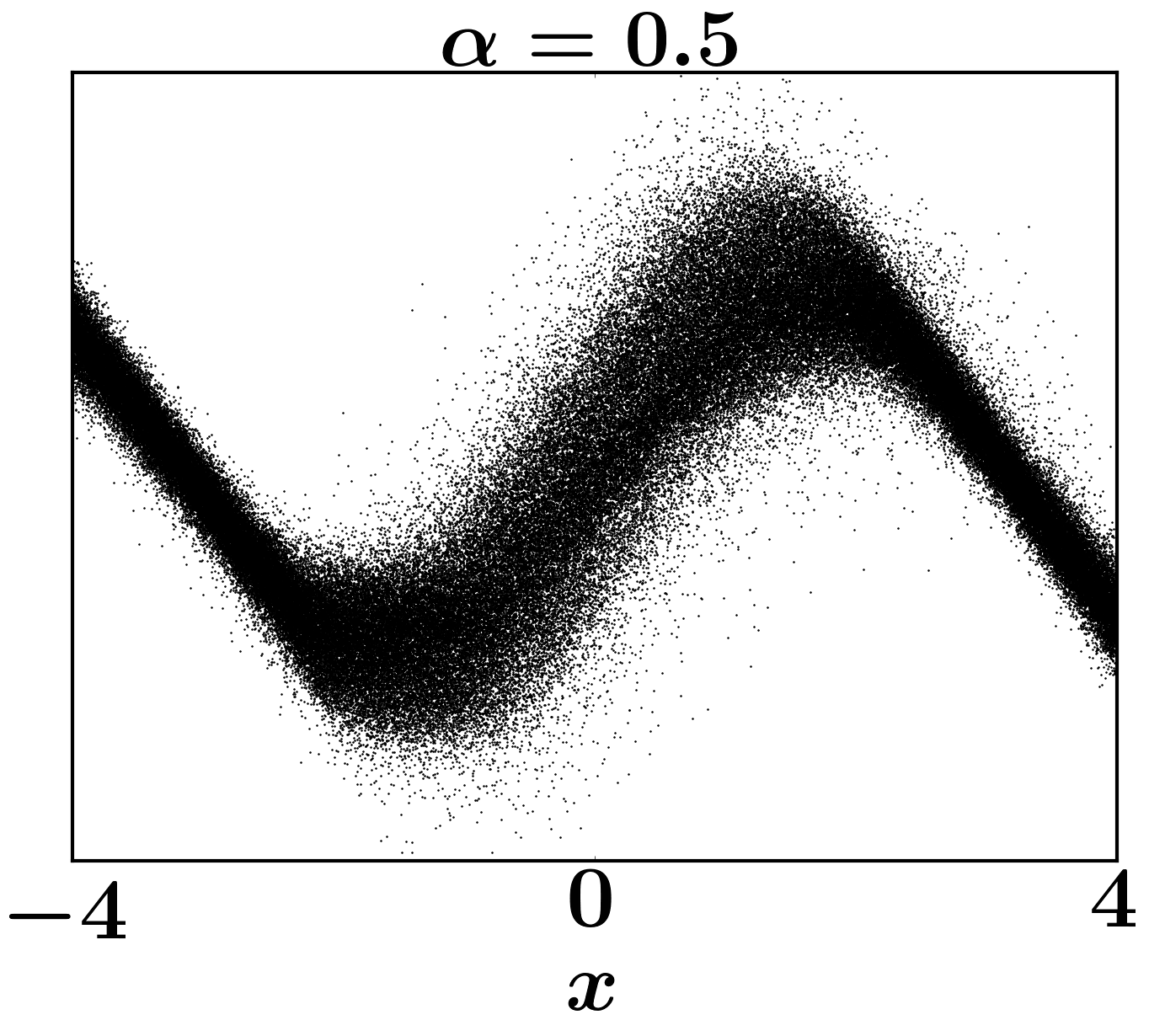
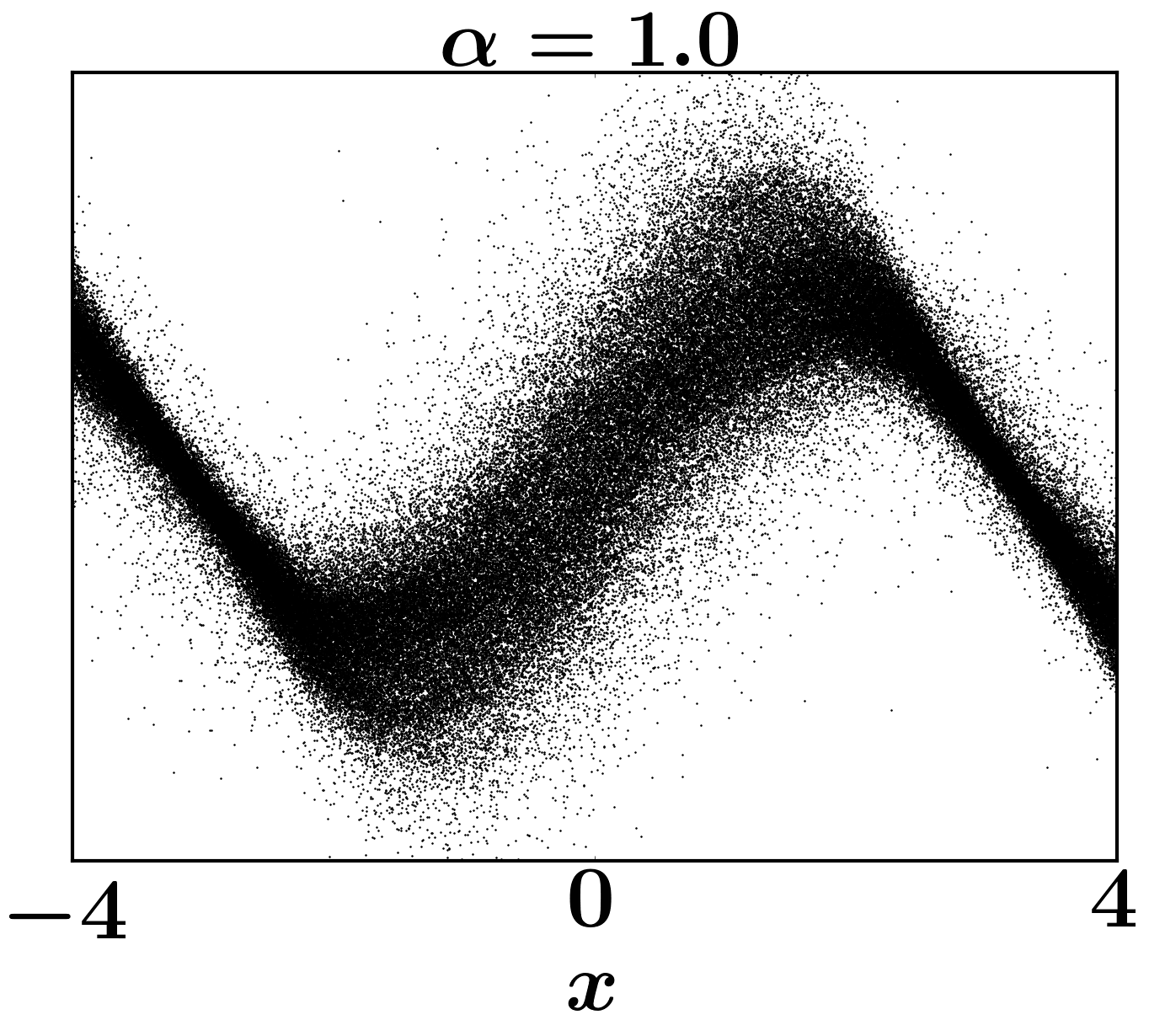
The plots in the 3rd and 4th columns of Figure 5 show the predictions obtained with $\alpha=0.5$ and $\alpha=1.0$, respectively. In these cases, the predictive distribution is able to capture the bimodality in the first problem and the heteroskedasticity pattern in the second problem in both cases The plots in the 2nd column of Figure 5 show the predictions obtained with VB, which converges to suboptimal solutions in which the predictive distribution has a single mode (in the first problem) or is homoskedastic (in the second problem). Tables 3 and 4 show the average test RMSE and log-likelihood obtained by each method on each problem.

These results show that Bayesian neural networks trained with $\alpha=0.5$ or $\alpha=1.0$ are more robust than VB and can still model complex predictive distributions, which may be multimodal and heteroskedastic, even when $q(\mathbf{z})$ is not learned and is instead kept fixed to the prior $p(\mathbf{z})$. By contrast, VB fails to capture complex stochastic patterns in this setting.

Method	RMSE	Log-likelihood
VB	5.12	-3.05
$\alpha=0.5$	5.14	-2.10
$\alpha=1.0$	5.15	-2.11

Table 3: Test error and log-likelihood for the bi-modal prediction problem.

Method	RMSE	Log-likelihood
VB	1.88	-2.05
$\alpha=0.5$	1.89	-1.78
$\alpha=1.0$	1.94	-1.98

Table 4: Test error and log-likelihood for the heteroskedastic prediction problem.

Appendix B Methods

In the experiments we compare to the following methods:

Standard MLP.

The standard multi-layer preceptron (MLP) is equivalent to our BNNs, but does not have uncertainty over the weight $\mathcal{W}$ and does not include any stochastic inputs. We train this method using early stopping on a subset of the training data. When we perform roll-outs using algorithm 1, the predictions of the MLP are made stochastic by adding Gaussian noise to its output. The noise variance is fixed by maximum likelihood on some validation data after model training.

Variational Bayes (VB).

The most prominent approach in training modern BNNs is to optimize the variational lower bound (Blundell et al., 2015; Houthooft et al., 2016; Gal et al., 2016). This is in practice equivalent to $\alpha$-divergence minimization when $\alpha\to 0$ (Hernández-Lobato et al., 2016). In our experiments we use $\alpha$-divergence minimization with $\alpha=10^{-6}$ to implement this method.

Gaussian Processes (GPs).

Gaussian Processes have recently been used for policy search under the name of PILCO (Deisenroth & Rasmussen, 2011). For each dimension of the target variables, we fit a different sparse GP using the FITC approximation (Snelson & Ghahramani, 2005). In particular, each sparse GP is trained using $150$ inducing inputs by using the method stochastic expectation propagation (Bui et al., 2016). After this training process we approximate the sparse GP by using a feature expansion with random basis functions (see supplementary material of Hernández-Lobato et al. 2014). This allows us to draw samples from the GP posterior distribution over functions, enabling the use of Algorithm 1 for policy training. Note that PILCO will instead moment-match at every roll-out step as it works by propagating Gaussian distributions. However, in our experiments we obtained better performance by avoiding the moment matching step with the aforementioned approximation based on random basis functions.

Particle Swarm Optimization Policy(PSO-P).

We use this method to estimate an upper bound for reward performance. PSO-P is a model predictive control (MPC) method that uses the true dynamics when applicable (Hein et al., 2016a). For a given state $\mathbf{s}_{t}$, the best action is selected using the standard receding horizon approach on the real environment. Note that this is not a benchmark method to compare to, we use it instead as an indicator of what the best possible reward can be achieved for a fixed planning horizon $T$.

Appendix C Model Parameters

For all tasks we will use a standard MLP with two hidden layer with $20$ hidden units each as policy representation. The activation functions for the hidden units are rectifiers: ${\varphi(x)=\max(x,0)}$. If present, bounding of the actions is realized using the $\tanh$ activation function on the outputs of the policy. All models based on neural network will share the same hyperparameter. We use ADAM as learning algorithm in all tasks.

WetChicken

The neural network models are set to 2 hidden layers and 20 hidden units per layer. We use 2500 random state transitions for training. We found that assuming no observation noise by setting $\Gamma$ to a constant of $10^{-5}$ helped the models converge to lower energy values.

For policy training we use a horizon of size $T=5$ and optimize the policy network for $100$ epochs, averaging over $K=20$ samples in each gradient update, with mini-batches of size $10$ and learning rate set to $10^{-5}$.

Turbine

The world model and the BNNs have two hidden layers with $50$ hidden units each. For policy training and world-model evaluation we perform a roll-out with horizon $T=20$. For learning the policy we use minibaches of size $10$ and draw $K=10$ samples from $q$.

Industrial Benchmark

For the neural network models we use two hidden layers with $75$ hidden units.We use a horizon of $T=75$, training for $500$ epochs with batches of size $50$ and $K=25$ samples for each rollout.

Appendix D Computational Complexity

Model Training

All models were trained using theano and a single GPU. Training the standard neural network is fast, the training time for this method was between 5 - 20 minutes, depending on data set size and dimensionality of the benchmark. In theano, the computational graph of the BNNs is similar to that of an ensemble of standard neural networks. The training time for the BNNs varied between 30 minutes to 5 hours depending on data size and dimensionality of benchmark. The sparse Gaussian Process was optimized using an expectation propagation algorithm and after training, it was approximated with a Bayesian linear model with fixed basis functions whose weights are initialized randomly (see Appendix B). We choose the inducing points in the GPs and the number of training epochs for these models so that the resulting training time was comparable to that of the BNNs.

Policy Search

For policy training we used a single CPU. All methods are of similar complexity as they are all trained using Algorithm 1. Depending on the horizon, data set size and network topology, training took between 20 minutes (Wet-Chicken, $T=5$), 3-4 hours (Turbine, $T=20$) and 14-16 hours (industrial benchmark, $T=75$).

References

- Bertsekas (2002) D.P. Bertsekas. Dynamic Programming and Optimal Control. Athena Scientific optimization and computation series. 2002. ISBN 9781886529083.
- Blundell et al. (2015) Charles Blundell, Julien Cornebise, Koray Kavukcuoglu, and Daan Wierstra. Weight uncertainty in neural networks. In ICML, pp. 1613–1622, 2015.
- Bui et al. (2016) Thang D Bui, Daniel Hernández-Lobato, Yingzhen Li, José Miguel Hernández-Lobato, and Richard E Turner. Deep Gaussian processes for regression using approximate expectation propagation. In ICML, pp. 1472–1481, 2016.
- Deisenroth & Rasmussen (2011) Marc Deisenroth and Carl E Rasmussen. PILCO: A model-based and data-efficient approach to policy search. In ICML, pp. 465–472, 2011.
- Deisenroth et al. (2013) Marc Peter Deisenroth, Gerhard Neumann, and Jan Peters. A survey on policy search for robotics. Foundations and Trends in Robotics, 2:1–142, 2013.
- Draeger et al. (1995) A. Draeger, S. Engell, and H. Ranke. Model predictive control using neural networks. IEEE Control Systems, 15:61–66, 1995.
- Gal et al. (2016) Yarin Gal, Rowan Mcallister, and Carl Rasmussen. Improving PILCO with Bayesian neural networks dynamics models. In Data-Efficient Machine Learning workshop, ICML, 2016.
- Gu et al. (2016) Shixiang Gu, Timothy Lillicrap, Ilya Sutskever, and Sergey Levine. Continuous deep q-learning with model-based acceleration. arXiv preprint arXiv:1603.00748, 2016.
- Hans & Udluft (2009) Alexander Hans and Steffen Udluft. Efficient uncertainty propagation for reinforcement learning with limited data. In ICANN, pp. 70–79. Springer, 2009.
- Hein et al. (2016a) Daniel Hein, Alexander Hentschel, Thomas A Runkler, and Steffen Udluft. Reinforcement learning with particle swarm optimization policy (PSO-P) in continuous state and action spaces. IJSIR, 7:23–42, 2016a.
- Hein et al. (2016b) Daniel Hein, Alexander Hentschel, Volkmar Sterzing, Michel Tokic, and Steffen Udluft. Introduction to the" industrial benchmark". arXiv preprint arXiv:1610.03793, 2016b.
- Hernández-Lobato et al. (2014) José Miguel Hernández-Lobato, Matthew W Hoffman, and Zoubin Ghahramani. Predictive entropy search for efficient global optimization of black-box functions. In NIPS, pp. 918–926, 2014.
- Hernández-Lobato et al. (2016) José Miguel Hernández-Lobato, Yingzhen Li, Mark Rowland, Daniel Hernández-Lobato, Thang Bui, and Richard E Turner. Black-box -divergence minimization. In ICML, pp. 1511–1520, 2016.
- Houthooft et al. (2016) Rein Houthooft, Xi Chen, Yan Duan, John Schulman, Filip De Turck, and Pieter Abbeel. VIME: Variational information maximizing exploration. In NIPS, pp. 1109–1117, 2016.
- Kingma et al. (2015) Diederik P Kingma, Tim Salimans, and Max Welling. Variational dropout and the local reparameterization trick. In NIPS, pp. 2575–2583, 2015.
- Ko et al. (2007) Jonathan Ko, Daniel J Klein, Dieter Fox, and Dirk Haehnel. Gaussian processes and reinforcement learning for identification and control of an autonomous blimp. In IEEE Robotics and Automation, pp. 742–747, 2007.
- Minka (2005) Tom Minka. Divergence measures and message passing. Technical report, Microsoft Research, 2005.
- Peters & Schaal (2006) Jan Peters and Stefan Schaal. Policy gradient methods for robotics. In IROS, pp. 2219–2225, 2006.
- Peters & Schaal (2008) Jan Peters and Stefan Schaal. Reinforcement learning of motor skills with policy gradients. Neural networks, 21:682–697, 2008.
- Rasmussen et al. (2003) Carl Edward Rasmussen, Malte Kuss, et al. Gaussian processes in reinforcement learning. In NIPS, pp. 751–758, 2003.
- Schaefer et al. (2007) Anton Maximilian Schaefer, Steffen Udluft, and Hans-Georg Zimmermann. The recurrent control neural network. In ESANN, pp. 319–324, 2007.
- Snelson & Ghahramani (2005) Edward Snelson and Zoubin Ghahramani. Sparse Gaussian processes using pseudo-inputs. In NIPS, pp. 1257–1264, 2005.
- (23) Theano Development Team. Theano: A Python framework for fast computation of mathematical expressions. arXiv e-print abs/1605.02688.
- Tresp (1994) V. Tresp. The wet game of chicken. Technical report, 1994.
- Wahlberg (1991) Bo Wahlberg. System identification using Laguerre models. IEEE Transactions on Automatic Control, 36:551–562, 1991.
- Wainwright & Jordan (2008) M. J. Wainwright and M. I. Jordan. Graphical models, exponential families, and variational inference. Foundations and Trends in Machine Learning, 1:1–305, 2008.
- Wang & Dietterich (2003) Xin Wang and Thomas G Dietterich. Model-based policy gradient reinforcement learning. In ICML, pp. 776–783, 2003.
- Watter et al. (2015) Manuel Watter, Jost Springenberg, Joschka Boedecker, and Martin Riedmiller. Embed to control: A locally linear latent dynamics model for control from raw images. In NIPS, pp. 2728–2736, 2015.
Appendix A Robustness of and when is not learned