Stable and accurate interface capturing advection schemes

Abstract

In this paper, stable and “low-diffusive” multidimensional interface capturing (IC) schemes using slope limiters are discussed. It is known that direction-by-direction slope-limited MUSCL schemes create geometrical artefacts and thus return a poor accuracy. We here focus on this particular issue and show that the reconstruction of gradient directions are an important factor of accuracy. The use of a multidimensional limiting process (MLP) added with an adequate time integration scheme leads to an artefact-free and instability-free interface capturing (IC) approach. Numerical experiments like the reference Kothe-Rider forward-backward advection case show the accuracy of the approach. We also show that the approach can be extended to the more complex compressible multimaterial hydrodynamics case, with potentially an arbitrary number of fluids. We also believe that this approach is appropriate for multicore/manycore architecture because of its SIMD feature, which may be another asset compared to interface reconstruction approaches.

1 Introduction and motivation

Nowadays there are recognized computational methods to numerically simulate material interfaces or moving free boundaries. Among the well-known approaches, let us mention the levelset approach pioneered by Osher-Sethian [28], the family of interface reconstructions (IR) algorithms [6, 5] that can be more or less sophisticated (moments-of-fluid approaches [5] being the most sophisticated), and diffuse interface capturing (IC) methods [36, 38, 8, 9, 10, 2, 26, 7, 18, 13, 27, 31]. Each of these methods both show advantages and drawback, and thus are more or less suitable for different problems according to the kind of application, the expected properties and the quantities of interest to compute. For example, if conservation properties are mandatory, levelset methods are not the right candidate family: even if today we find volume conservative levelset methods, mass conservation may not be strictly fulfilled, what can be not accurate enough for some highly compressible flows or flows with high ratios of density. After decades of sustained developments and research in this fields, interface capturing (IC) methods are still an active field of investigation (see the recent references [8, 9, 10, 2, 7, 29, 31, 40]). They can show advantages like a natural extension to an arbitrary number of fluids, phases of materials, the possibility to deal with complex topologies and configurations (triple points, …) in a rather easy way, the simplicity of code development, debugging and optimization.

There is also another feature not to forget: the compute performance of the methods, especially for multicore or manycore parallel computer architectures that appear to be the current and future driving hardware trend. Multicore/manycore processors allow of speedups only if algorithms are suitable for that. Key factors of performance are typically a well-balanced operational intensity, data coalescence in memory, cache blocking, processor occupancy and SIMD feature of the algorithms [30]. We advocate the idea that today a good computational approach is a good trade-off between numerical analysis requirements (like order of accuracy and stability), generalization/flexibility property and fast or practical implementation features. Our experience in computational methods, performance evaluation and performance modeling [30] make us believe that interface capturing schemes are good candidates for these performance issues, ready to fulfil most of these performance factors.

As a summary, we look for interface capturing methods that share the following properties:

• numerical stability and low-diffusive aspect;

• SIMD-type algorithms;

• simple coding and debugging;

• relatively easy extension to an arbitrary number of materials;

• relatively easy extension to three-dimensional problems;

• natural extension to unstructured meshes;

• relatively simple prediction of computing performance.

This paper more focuses on stability, low-diffusive feature and accuracy of interface capturing methods, but we keep in mind all the above requirements. The paper is organized as follows. In section 2, we will test standard MUSCL slope limiter-based finite volume schemes for interface capturing and will show a set of artefacts and instabilities by numerical evidence. In section 3, we will provide some elements of analysis about these artefacts. We will enumerate the requirements for a good interface capturing scheme in section 4 and then discuss multidimensional limiting process methods in section 5. Numerical experiments in section 6 will confirm both stability and accuracy of our approach and considerations for the extension toward compressible multimaterial hydrodynamics will be given in section 7.

Mathematical setup and notations.

We need to describe free boundaries moving into a continuous medium described in a bounded spatial domain $\Omega\subset\mathbb{R}^{d}$, $d\in\{2,3\}$. Let us denote by $\bm{u}$ the vector field on the underlying transport phenomenon. As a first step and for simplicity let us assume that the vector field only depends on space $\bm{x}$ and not on time $t$. We add the following regularity assumptions on the vector field : $\bm{u}\in[W^{1,\infty}(\Omega)]^{d}$ and $\bm{u}$ is divergence-free, i.e. $\nabla\cdot\bm{u}=0$ almost everywhere. Then any quantity $z$ solution the pure advection equation

$$D_{t}z=\partial_{t}z+\bm{u}\cdot\nabla z=0,$$

is also solution of the conservation law

$$\partial_{t}z+\nabla\cdot(z\bm{u})=0.$$

Variable $z$ is a conservative variable in the sense that

$$\frac{d}{dt}\int_{V_{t}}z(\bm{x},t)\,d\bm{x}=0$$ (1)

for any measurable set $V_{t}$ which is transported itself by the vector field $\bm{u}$ so that the “mass” quantity

$$m_{t}=\int_{V_{t}}z(\bm{x},t)\,d\bm{x}$$

is conserved through time $t$. Because we are dealing with the capture of moving free boundaries, we here consider discontinuous solutions $z$ with values only in $\{0,1\}$ at the continuous level. Let us remark that, from the Reynolds transport theorem,

$$\frac{d}{dt}|V_{t}|=\frac{d}{dt}\int_{V_{t}}1\,d\bm{x}=\int_{V_{t}}\{\partial_{t}1+\nabla\cdot\bm{u}\}\,dx=0,$$

thus there is volume conservation for a divergence-free velocity field. So conservation of volume and conservation of “mass” are equivalent in this case. At the discrete level, we want to keep the conservation properties, so finite volumes methods are the natural candidates for that. To set the ideas, let us consider a two-dimensional rectangular bounded domain $\Omega$ and a cartesian discretization mesh with uniform mesh steps $h_{x}=h_{y}=h$ leading to square finite volumes. Let us use $K$ as generic notation of a given finite volume, $A$ an edge of volume $K$, the vector $\bm{\nu}_{A}$ being the outer normal unit vector to $A$ pointing out of $K$. We look for finite volume schemes (here written in semi-discrete form – time discretization will be discussed later) in the form

$$\frac{dz_{K}}{dt}=-\frac{1}{|K|}\sum_{A\subset\partial K}|A|\,z_{A}\,\bm{u}_{A}\cdot\bm{\nu}_{A}$$ (2)

where $z_{A}$ (resp. $\bm{u}_{A}$) denotes a certain value of $z$ (resp. $\bm{u}$) at the midpoint of edge $A$. The quantity

$$\text{div}^{h}_{K}(\bm{u}z)=\frac{1}{|K|}\sum_{A\subset\partial K}|A|\,z_{A}\,\bm{u}_{A}\cdot\bm{\nu}_{A}$$

is nothing else but a discrete divergence operator of the vector flux $\bm{f}=\bm{u}z$ into the cell $K$. Because we deal with divergence-free velocity vectors, we may chose $(\bm{u}_{A}\cdot\bm{\nu}_{A})$ in order to get the discrete equivalent

$$\sum_{A\subset\partial K}|A|\bm{u}_{A}\cdot\bm{\nu}_{A}=0.$$

For that it is sufficient to consider mean values $\bm{u}_{A}\cdot\bm{\nu}_{A}$ computed as

$$\bm{u}_{A}\cdot\nu_{A}=\frac{1}{|A|}\int_{A}\bm{u}\cdot\bm{\nu}_{A}\,d\sigma.$$

In summary, we have defined a numerical normal flux

$$\phi_{A}=(\bm{u}_{A}\cdot\bm{\nu}_{A})\,z_{A}$$

across the edge $A$ in the direction $\bm{\nu}_{A}$. We now have only to correctly chose and compute the edge quantity $z_{A}$ in order to get a stable and low-diffusive time advance scheme.

2 Testing MUSCL slope limiter-based schemes for interface transport

2.1 One-dimensional case

Here we begin with a short introduction and summary of well-known second-order finite volume solvers using MUSCL reconstruction for the one-dimensional advection equation

$$\partial_{t}z+\partial_{x}(uz)=0$$

for a given constant real number $\bm{u}\neq 0$. Spatially semi-discrete conservative schemes for a uniform grid read

$$\frac{dz_{j}}{dt}=-\frac{\psi_{j+1/2}-\psi_{j-1/2}}{h},\quad\quad j\in\mathbb{Z},$$ (3)

where $h$ denotes a constant spatial step of the grid $\{x_{j}=jh\}_{j}$, $j\in\mathbb{Z}$, and the quantities $\psi_{j+1/2}$ are numerical fluxes between cells $j$ and $(j+1)$. The fluxes are at least consistent with the physical (linear) flux $f(z)=uz$ to get first-order accuracy. Slope-based MUSCL reconstructions methods try to locally reconstruct a slope for each cell by finite differences and then limit the slopes for total variation diminishing (TVD) stability purposes [16, 37]. Without time discretization, the upwind numerical fluxes generally are written in viscous form

$$\psi_{j+1/2}=\frac{f(z_{j+1/2}^{-})+f(z_{j+1/2}^{+})}{2}-\frac{1}{2}|u|(z_{j+1/2}^{+}-z_{j+1/2}^{-}),$$ (4)

where $z_{j+1/2}^{-}$ and $z_{j+1/2}^{+}$ are left and right extrapolation values at location $x_{j+1/2}=(j+1/2)h$ respectively, according to a conservative piecewise linear approximation

$$z(x)=z_{j}+s_{j}(x-x_{j}),\quad\quad x\in(x_{j-1/2},x_{j+1/2}),$$

and then

$$z_{j+1/2}^{-}=z_{j}+\frac{h}{2}s_{j},\quad z_{j-1/2}^{+}=z_{j}-\frac{h}{2}s_{j}.$$

The numerical flux (4) can be rewritten

$$\psi_{j+1/2}=\left\{\begin{array}[]{l}u\,z_{j+1/2}^{-}\quad\text{if }u\geq 0,\\[4.73611pt] u\,z_{z+1/2}^{+}\quad\text{if }u\leq 0\end{array}\right.$$

and clearly shows the underlying upwind process. In the slope limitation theory, one tries to reconstruct and limit a slope according to some requirement like second-order accuracy and TVD property for the scheme. Cell-centered three-point slope reconstructions have the form

$$s_{j}=\frac{1}{h}\,\phi(\Delta z_{j}^{-},\Delta z_{j}^{+})$$

with $\Delta z_{j}^{-}=z_{j}-z_{j-1}$, $\Delta z_{j}^{+}=z_{j+1}-z_{j}$, and $\phi$ is a limiter function. Among, standard limiter functions $\phi$, let us mention the “compressive” ones that will be used in the sequel of the paper:

• Superbee limiter [33]:

  $$\phi^{S}(a,b)=\text{sgn}(a)\,(ab\geq 0)\,\max[\min(|a|,2|b|),\min(2|a|,|b|)];$$

• a more compressive limiter (referred to as the “overbee” limiter in this paper, used for example in [31]):

  $$\phi^{O}(a,b)=2\,\text{sgn}(a)\,(ab\geq 0)\,\min(|a|,|b|);$$

Superbee limiters allow for second-order reconstruction because of the property $\phi^{S}(a,a)=a$ and regularity whereas the “overbee” limiter overestimates the slopes:

$$\phi^{O}(a,a)=2a\quad\forall a.$$

The overbee limiter is a priori intended for use with step-shaped or staircase functions only. Although being overcompressive, it leads to a $L^{\infty}$-stable scheme under CFL conditions less than $1/2$.

For full discretized numerical schemes (by the explicit Euler scheme for example), there are also CFL-dependent limiter functions, like Roe’s Ultrabee limiter [33], depending on the Courant number $\nu=|u|\Delta t/h$, with $\Delta t$ as time step. Després and Lagoutière [8] in their construction of the most compressive stable scheme for interface advection (known as limited-downwind approach) have reinterpreted their construction in terms of flux limiter and then retrieve the Ultrabee limiting process.

As an illustration, let us consider the simple test case of transport of the initial top hat function

$$z^{0}(x)=1_{(0\,\leq\,x\,\leq\,1/2)}(x)$$

on the interval $\Omega=(0,1)$ with periodic boundary conditions, $u=1$. Let us use a uniform grid made of 250 points. We implement the MUSCL scheme using the overbee limiter with the explicit Euler time discretization. We use a Courant number $\nu=0.35$. Final time is $t=5/4$. On figure , the discrete solution at final time is plotted. We can observe a quite good capture of the discontinuities “at the eye norm”. Looking more deeply at the viscous profile by visualizing the logarithm of the quantity $z(1-z)$ that is representative of the smearing rate, one can observe a smearing of about 10 points that decreases in log scale with a cutoff at $10^{-10}$. Than can be be simply explained with the following configuration: consider $u>0$, discrete values $z_{j-1}^{n}=1$, $z_{j}^{n}<1$ close to 1 and $z_{j+1}^{n}$ close to 0. Applying the MUSCL/overbee limiter under this configuration clearly gives

$$z_{j}^{n+1}-1 = z_{j}^{n}-1-\nu([z_{j}^{n}+\frac{1}{2}\,2(z_{j}^{n}-z_{j-1}^{n})]-1)$$

$$= (1-2\nu)(z_{j}^{n}-1).$$

Stability is ensured under the CFL condition $\nu\leq 1/2$, but for $\nu<1/2$, the have a geometric series with factor $(1-2\nu)\in(0,1)$. The convergence rate toward 1 is CFL-dependent and can be rather small for small Courant values. The only way to avoid this is to use compressive CFL-dependent limiters like the Ultrabee one and is at the source of Roe’s construction [33] or Després-Lagoutière in their construction of limited-downwind antidiffusive approach [8]. Another important thing to notice in this experiment is the asymptotic bound in time of the smearing rate, i.e.

$$t\mapsto\max_{s\in(0,t)}\,\int_{0}^{1}[z(1-z)](s)\,ds$$

is bounded (figure 1b), which states in some sense the low-diffusive feature of the approach.

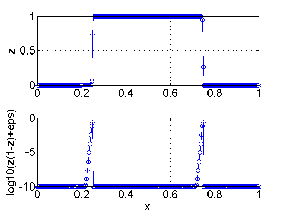
(a) Profile of $z$ and $\log_{10}(z(1-z)+10^{-10})$ at final time.

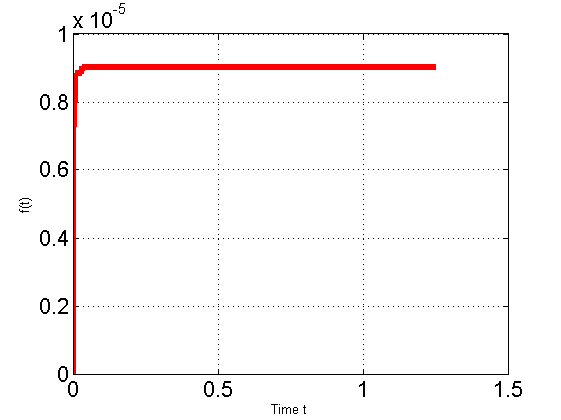
(b) History of quantity
$t\mapsto\max_{s\in(0,t)}\,\|[z(1-z)](s)\|_{L^{1}(0,1)}$.

Figure 1: Numerical experiment: assessment of numerical diffusion and smearing of step-shaped functions when the overbee limiter is used. One can observe a smearing of a few points “at the eye norm”, and about $O(10)$ point in log scale. Time evolution of the smearing rate $t\mapsto\max_{s\in(0,t)}\,\int_{0}^{1}(z(1-z))(x,s)\,dx$ shows an asymptotic bound.

2.2 Artefacts and instabilities encountered for multidimensional problems

For multidimensional problems, the state of theoretical analysis of slope limiters is still nowadays quasi-open or quite poor. Total variation theory for example cannot be extended for multidimensional problems. Anyway, we would like to experimentally observe the behavior of direction-by-direction slope limiters on a natural multidimensional extension of the MUSCL reconstruction upwind scheme.

Let us define three “simple” advection cases. First, consider the square domain $\Omega=(-1,1)^{2}$ discretized with a cartesian grid made square of edge length $h$. Consider also periodic boundary conditions. As initial data, let us define a disk-shaped hat function

$$z(\bm{x},t=0)=1_{(x^{2}+y^{2}<0.2)}(\bm{x}).$$

and consider a uniform velocity field generated by the diagonal advection vector $\bm{u}=(1,1)$. For the advection scheme, consider the upwind MUSCL approach with the direction-by-direction slope limiter Superbee and a Runge-Kutta RK2 time integration for the time advance scheme. We use a CFL number of 0.2 . Final time of numerical simulation is $t=10$, the disk-shaped function should be retrieved at final time at its initial location. The results are plotted in figure 2. We observe that the disk interface degenerates and artificially evolves in time toward an octagon-shaped boundary, as already noticed by Després and Lagoutière in [9] when the limited-downwind anti-dissipative approach is used. The numerical scheme does not create new extrema and is locally monotonicity-preserving, but some accuracy is lost and it is disappointing to state that the error is $O(1)$ at final time. Some error is accumulating in time. Let us also claim that a directional splitting strategy does not solve this artefact problem.

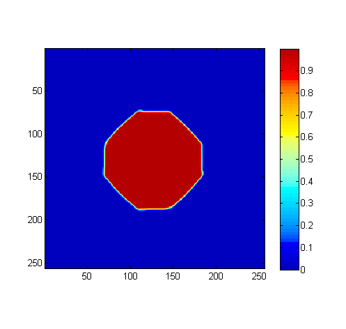
(a) Colored representation of the solution $z$.

(b) Colored representation of $z(1-z)$.

Figure 2: Disk advected into a uniform vector field $\bm{u}=(1,1)$ in the domain $[-1,1]^{2}$ (periodic boundary conditions) which evolves toward an non-physical octagon-shaped form. Clearly the error is $O(1)$. Discrete solution at final time $t=10$, cartesian grid $256^{2}$. Slope limiters are direction-by-direction superbee limiters. RK2 is used as time integrator and the CFL number is $0.3$.

As a second test case, let us still consider the same geometry with periodic boundary conditions, but now with a pure rotating velocity field defined by $\bm{u}(\bm{x})=(-y,x)$. As initial condition, consider the disk-shaped function

$$z(\bm{x},t=0)=1_{\left((x-\frac{1}{2})^{2}+y^{2}\,<\,0.15\right)}(\bm{x}).$$

Now the computational grid is $512^{2}$. We still use the MUSCL approach with the Superbee limiter and an explicit Euler time integration. We use a CFL number of 0.3. Results are shown in figure 3 at final time $t=2\pi$ corresponding to a complete revolution of the disk in the domain. One can observe some free boundary zigzag-shaped instabilities in region where the local Courant number is rather large. Zigzag instabilities are a recurrent problem already reported in the literature for interface capturing methods [26]. A way to fix the problem is to use far smaller CFL numbers, but of course at the price of a weaker performance and a greater diffusivity.

(a) Colored representation of the solution $z$.

(b) Colored representation of $z(1-z)$.

Figure 3: Pure rotation of an disk into a rotating velocity vector field $\bm{u}(\bm{x})=(-y,x)$. Discrete solution at final time $t=2\pi$, cartesian grid $512^{2}$. One can observe spurious “zigzag” instabilities at the interface. Slope limiters are direction-by-direction Superbee limiters. The Euler explicit scheme is used as time integrator and the CFL number is $0.3$.

Finally, consider a third case of steady discontinuity aligned with the uniform velocity vector field (but not with the grid directions). Consider the spatial domain $\Omega=(0,1)^{2}$ discretized by a Cartesian grid $200\times 200$ with Neumann boundary conditions, a uniform velocity field generated by the vector $\bm{u}=(2,1)$ and an initial data made up of a discontinuity aligned with the velocity field :

$$z(\bm{x},t=0)=1_{(y\,\leq\,x/2)}(x,y).$$

The initial data is projected over piecewise constant functions, with “mixed cells” that discretize the interface. Because of the velocity vector $\bm{u}=(2,1)$, $z$ values into mixed cells actually are $1/4$ or $3/4$ (see also the next section for more details). The CFL number is 0.25 and the overbee limiter is used. As time discretization, of the first-order explicit Euler scheme is used. Final time is $t=2$. As observed on figure 4, the initial discontinuity becomes unstable and zigzag modes appear again. Zigzag instabilities tend to be amplified downstream and moreover produce a spurious unstationary field.

(a) Colored representation of the solution $z$.

(b) Colored representation of $z(1-z)$.

Figure 4: Steady discontinuity problem. Expected steady discontinuous solution with interface aligned with the velocity direction $(\bm{u}\cdot\nabla z=0)$. For rather big values of Courant numbers (less than one), one can observe the emergence of zigzag instabilities, even when the expected discrete steady state is used as initial data. Limiter function here is the so-called compressive overbee limiter. We believe that the source of instability is due to a bad evaluation of the gradient direction, creating over/under-evaluations of the directional convective fluxes.

3 Elements of analysis

3.1 Effects of one-dimensional slope limiters

From the results of the previous section, as a summary we observe two kinds of spurious solutions: i) stable evolution toward a non-physical solution (no instability) with privileged directions (grid-aligned directions, diagonal); ii) appearance of zigzag-shaped interface instabilities.

Regarding i), there is a loss of accuracy in this case. Of course the analysis of the determination of the order of accuracy is quite hard to achieve because the loss of accuracy of course occurs at locations where the solution is exactly non-smooth (actually discontinuous). In any event, let us try to find some expected consistency or accuracy conditions in particular cases.

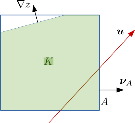
Figure 5: Geometrical elements and privileged directions for the interface advection problem

In the discrete advection problem, we have privileged directions (see figure 5): first the unit vector $\bm{\nu}_{A}$ which is normal to the edge $A$, then the direction of advection (given by $\bm{u}$) and the gradient $\nabla z$.

Let us consider a nontrivial uniform velocity field $\bm{u}(\bm{x})=\text{Cst}=\bm{u}$, $|\bm{u}|\neq 0$, and a stationary solution $z$ of the problem. Then $z$ is solution of $\bm{u}\cdot\nabla z=0$, or

$$\nabla\cdot(\bm{u}z)=0$$

in conservative form. If a stationary interface exists, then it is parallel to the line of velocity directions. Let us see what happen at the discrete level. Recall the discrete divergence operator

$$\text{div}^{h}_{K}(\bm{u}z)=\frac{1}{|K|}\sum_{A\subset\partial K}|A|\,z_{A}\,\bm{u}_{A}\cdot\bm{\nu}_{A}.$$

For a uniform velocity field $\bm{u}$, this reduces to

$$\text{div}^{h}_{K}(\bm{u}z)=\bm{u}\cdot\left(\frac{1}{|K|}\sum_{A\subset\partial K}|A|\,z_{A}\,\bm{\nu}_{A}\right).$$ (5)

In the above expression we recognize a discrete gradient operator for $z$ :

$$\text{grad}_{K}^{h}(z)=\frac{1}{|K|}\sum_{A\subset\partial K}|A|\,z_{A}\,\bm{\nu}_{A}.$$

Assume that locally we have the linear reconstruction

$$\mathscr{I}z(\bm{x})=z_{K}+\bm{g}_{K}\cdot(\bm{x}-\bm{x}_{K}).$$ (6)

Putting (6) into (5) gives us

$$\text{div}^{h}_{K}(\bm{u}z)=\bm{u}\cdot\left(\frac{1}{|K|}\sum_{A\subset\partial K}|A|\,(z_{K}+\bm{g}_{K}\cdot(\bm{x}_{A}-\bm{x}_{K}))\,\bm{\nu}_{A}\right).$$

From the geometrical property

$$\sum_{A\subset\partial_{K}}|A|\bm{\nu}_{A}=\bm{0},$$

we get

$$\text{div}^{h}_{K}(\bm{u}z)=\bm{u}\cdot\left(\frac{1}{|K|}\sum_{A\subset\partial K}|A|\,\bm{\nu}_{A}(\bm{x}_{A}-\bm{x}_{K})^{T}\right)\bm{g}_{K}.$$

By applying Green’s formula, it is easy to check that

$$\frac{1}{|K|}\cdot\sum_{A\subset\partial K}|A|\,\bm{\nu}_{A}(\bm{x}_{A}-\bm{x}_{K})^{T}=\bm{I},$$

so that we find

$$\text{div}^{h}_{K}(\bm{u}z)=\bm{u}\cdot\bm{g}_{K}.$$

The question is to know whether $\bm{u}\cdot\bm{g}_{K}$ is close to zero or not. Of course, it depends on how $\bm{g}_{K}$ is computed, and in particular it depends on the choice of slope limiters. We have the following consistency results:

1. if $\bm{g}_{K}\propto\nabla z$, then we have $\text{div}^{h}_{K}(\bm{u}z)=0$ exactly, without error;

2. if $|\bm{g}_{K}\cdot\bm{u}|=O(h)$ then we have a first-order consistent formula;

3. if for some reason, there exists a constant $\beta>0$ which is independent of $h$, such that $|\bm{g}_{K}\cdot\bm{u}|>\beta$, we have a $0$-order consistency.

We claim that case 3) is exactly what occurs when direction-by-direction one-dimensional compressive slope limiters are used. In fact, one-dimensional slope limiters are used to limit the amplitude of gradients not to create new extrema and reproduce a derivative for smooth solutions, but may produce incorrect gradient directions in the multidimensional case and for non-smooth solutions.

In fact, reality is a little bit more tricky because reconstructed MUSCL upwind schemes also take into account the direction of advection by some upwind process. Let us consider the example given into figure 6. Let us still consider a uniform velocity field $\bm{u}=(2,1)^{T}$ and a continuous stationary interface aligned with $\bm{u}$. To derive a discrete solution, we project the continuous solution on piecewise constant solutions as suggested by the finite volume theory. One finds “mixed” cells with values either $1/4$ or $3/4$ that represent the interface at the discrete level. Let us assume the use of direction-by-direction slope limiter of type superbee (or ultrabee that would return the same result). The evaluation of the discrete divergence $\text{div}_{K}^{h}(\bm{u}z)$ involves a 9-point cross-shaped stencil as drawn in figure 6. On figure 6a), we focus on a mixed cell with value $3/4$. It is not hard to check that the discrete gradient at the center cell (without upwinding) is in this case $\bm{g}_{K}=\frac{1}{h}(1/2,-1/2)$ which is already a bad gradient. Taking into account the upwinding process, we find that

$$\text{div}_{K}^{h}(\bm{u}z)=\bm{u}\cdot(1/2,-1/2)^{T}/h=\frac{1}{2h}$$

This is clearly a bad value (it is expected to find 0), but moreover the value behaves like $O(h^{-1})$ ! At the neighbour mixed cell with discrete value $1/4$ (figure 6b)), the reconstructed gradient is $\bm{g}_{K}=\frac{1}{h}(1/2,-1/2)$, still incorrect. But, curiously, because of the upwind process, one can check that the resulting discrete divergence has the good value:

$$\text{div}_{K}^{h}(\bm{u}z)=\bm{u}\cdot(1/2,-1)^{T}/h=0.$$

Clearly, this example shows an imbalance of grid-aligned directional derivatives due to nonlinear limitations of the slope limiters, and the process is unable to predict the gradient directions correctly.

Still on this example, let us also mention the observed oscillatory behaviour of discrete gradients along with the interface line, which, is, in our opinion, probably another source of odd-even interface instability.

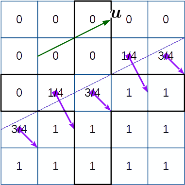
(a)  (b)

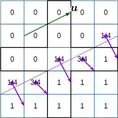
Figure 6: Computation of $\text{div}_{K}^{h}(\bm{u}z)$ for the following discrete solutions, using direction-by-direction slope limiters (superbee or ultrabee) at the center of each grid. The 9-point cross-shaped stencil for gradient reconstruction is plotted. Values of $z$ are given for each finite volume. The continuous interface is drawn in dashed line and is parallel to the uniform velocity vector $\bm{u}=(2,1)$. In case b) the reconstructed upwind MUSCL fluxes return the expected value $\text{div}_{K}^{h}(\bm{u}z)=\bm{u}\cdot(1/2,-1)/h=0$ while in case a) we find an incorrect value $\text{div}_{K}^{h}(\bm{u}z)=\bm{u}\cdot(1/2,-1/2)/h=\frac{1}{2h}=O(h^{-1})$. Let us also remark the spurious computation of zigzag-like gradient directions along the interface, which is be probably another source of numerical instability.

3.2 Behaviour of compressive limiters for interface normal vectors orthogonal to the velocity

Moreover, we claim that compressive limiters produce a loss of interface geometry accuracy for regions where $\nabla z\cdot\bm{u}$ is close to zero, i.e. when $\nabla z$ is almost orthogonal to $\bm{u}$, but not exactly.

As represented in figure 7 with a disk interface as example, the discrete profile of $z$ function in regions where $\nabla z\cdot\bm{u}\approx 0$ (top and bottom of the disk) and in the direction of velocity can be seen as a discretization of a smooth function, varying into $[0,1]$ because of the finite volume mean process. On figure 7 where $\bm{u}$ is aligned with the $x$-axis, applying one-dimensional too compressive limiters (superbee, overbee, ultrabee) will create spurious staircase-shaped functions in the top and bottom disk areas. Consequently, some of the initial geometry information will be lost. We believe that that this loss of accuracy is at the origin of spurious strange attractor shapes like octagons. To remedy this problem, one could imagine an hybrid slope limiter strategy that takes into account the direction deviation between $\nabla z$ and velocity $\bm{u}$. This is already proposed for example by Zhang et al. [42] in their so-called m-CICSAM method.

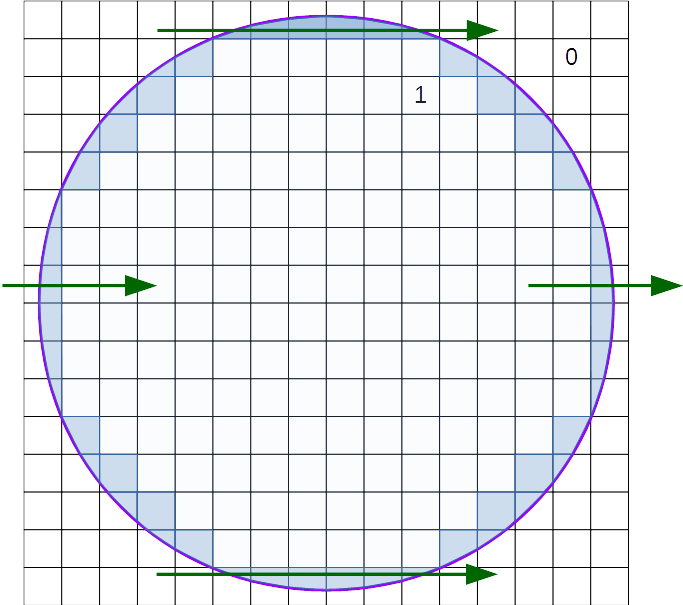
Figure 7: Mixed cells (in dark blue) when a disk-shaped solution is projected over piecewise constant solutions. For locations where $\nabla z$ is almost collinear to the velocity vector (in green), the discrete interface is essentially spread over one point whereas for areas with $\nabla z$ orthogonal or quasi-orthogonal to $\bm{u}$, the discrete $z$ profile in the velocity direction can be rather seen as a smooth varying function with values in $[0,1]$ and thus should be treated as a smooth function in this direction.

3.3 Influence of time discretization

Time discretization is also an important topic for interface capturing, not only for accuracy purposes but also especially for stability reasons. Time advance schemes for interface capturing are explicit. The simplest one is the one-step first-order Euler scheme that reads for the semi-discrete (in time) advection equation

$$\frac{z^{n+1}-z^{n}}{\Delta t}+\nabla\cdot(\bm{u}z^{n})=0.$$

It is very easy to derive the equivalent equation of the explicit first-order Euler scheme, i.e. the equation which is solved at the second-order accuracy by the Euler scheme, by Taylor expansions. One finds

$$\partial_{t}z+\nabla\cdot(\bm{u}z)=\frac{\Delta t}{2}\,\nabla\cdot(-(\bm{u}\otimes\bm{u})\,\nabla z).$$

The residual term at the right hand side is unfortunately an antidiffusive term that makes the associated problem ill-posed. Remark that the antidiffusion matrix $A=-\bm{u}\otimes\bm{u}$ is negative semi-definite with a kernel $\ker(A)=\text{span}(\bm{u}^{\bot})$. Here again, one can observe an anisotropic behaviour according to the direction of advection. Now because in our context $z$ is a nonsmooth function, actually higher-order terms in the Taylor expansion are also important (consider a scaling). Actually the true key word here is numerical stability. One has to use numerically stable time advance schemes in order to not produce spurious interface instabilities. We will see below in numerical experiments that even if spatial discretization in done properly, it will lead to linear instabilities evolving into nonlinear zigzag-shaped modes if the explicit Euler scheme is used, whereas second-order Runge-Kutta RK2 integrators eliminate these spurious instabilities.

4 Requirements for the interface capturing scheme

From the above numerical study and numerical analysis, we understand that accurate interface capturing methods must satisfy a set of requirements. We have identified the four following “constraints”:

1. The solver has to be overcompressive in the normal direction to the interface for low-diffusive properties;

2. the solver should be second-order accurate in directions tangent to the interface;

3. the gradient limiting process has to preserve the (unlimited) gradient direction $\nabla z$ (normal direction) for accuracy purposes;

4. high-order explicit time integrators having a reasonable stability region are required.

To fulfil the above requirements, our choice moves towards multidimensional limiting process (MLP) strategies ([40, 29]) that are generalizations of the limiters to the multidimensional case, thus allowing to keep control of the gradient direction. For time integrators we will simply use second-order Runge-Kutta RK2 schemes.

5 Multidimensional limiting process

Multidimensional limiting process or MLP has been introduced by different authors [40, 29] in order to provide an improved accuracy for multidimensional problems, especially for high-speed computational fluid dynamics. It is a natural extension of the one-dimensional slope-limiting process that takes into account the local neighbouring information for both gradient reconstruction and limitation. MLP can be formulated on general unstructured grids. In our paper, we will restrict to Cartesian grids even if the use of unstructured grids is possible. One of the difficulties in the multidimensional case is the definition of limitation criteria. Before MLP, older concepts like Local Extremum Diminishing (LED) proposed by Kuzmin and Turek [19, 20] are a substitute to the one-dimensional Total Variation Diminishing (TVD) tool. The idea is to limit a local reconstruction in order not to create new extrema, allowing for a $L^{\infty}$ diminishing property.

Here we decide to use MLP as a compressive multidimensional gradient reconstruction algorithm for interface capturing. Let us consider a two-dimensional Cartesian grid made of cells named $K_{i,j}$ indexed by $(i,j)$. The general process is the following:

1. First estimate the local cell discrete gradient $(\nabla^{h}z)_{i,j}$. This can be performed easily by means of approximation formulas or quadrature formulas in the case of finite volume approximation.

2. Consider piecewise-linear local approximations in the form:

   $$\mathscr{I}^{h}z(\bm{x})=z_{i,j}+\phi_{i,j}\,(\nabla^{h}z)_{i,j}(\bm{x}-\bm{x}_{i,j}).$$

   The coefficient $\phi_{i,j}$ will be a scalar gradient limiting factor.

3. Limit the slope in order not to create new local extrema at the cell corners, following a LED criterion [19]. Actually, for interface capturing we try to be as sharp as possible but without creating new local extrema, leading to a natural extension of the overbee slope limiter.

4. Reconstruct a piecewise constant sub-square solution: the piecewise linear local solution is projected onto a piecewise constant subcell solution over the four natural corner subsquares of each cell. This projection allows us to easily compute upwind numerical fluxes.

5. Finally compute the advective fluxes at the edges.

The involved geometric elements for performing the process are summarized on figure 8.

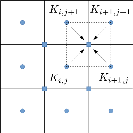
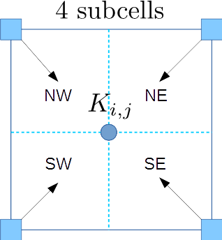
Figure 8: Geometric elements for multidimensional reconstruction and limiting process.

Now we give mathematical and technical details on both gradient prediction and limitation.

5.1 Gradient reconstruction predictor step

There are probably numerous ways to determine accurate gradients. In this work, we have chosen a finite volume approach to approximate the gradient from nearest neighbour cell information:

$$(\nabla z)_{ij} \approx \frac{1}{|K_{i,j}|}\int_{K_{i,j}}\nabla z(x,y)dx\,dy$$

$$= \frac{1}{|K_{i,j}|}\int_{\partial K_{i,j}}z\,\bm{\nu}\,d\sigma$$

$$= \frac{1}{|K_{i,j}|}\sum_{A\subset\partial K_{i,j}}\ \int_{A}z\,\bm{\nu}\,d\sigma.$$

We approximate each edge integral by second order accurate Simpson’s quadrature formula, i.e. for example for edge $A_{i+1/2,j}$:

$$\int_{A_{i+1/2,j}}z\,dy\approx\frac{h}{6}\,z_{i+1/2,j+1}+\frac{2h}{3}\,z_{i+1/2,j}+\,\frac{h}{6}z_{i+1/2,j-1}$$

where

$$z_{i+1/2,j}=\frac{z_{i,j}+z_{i+1,j}}{2}.$$

Summing up all the edge contributions, we get the 8-point scheme:

$$(\nabla^{h}z)_{i,j}=\frac{1}{h}\,\left(\begin{array}[]{c}\frac{1}{12}(z_{i+1,j+1}-z_{i-1,j+1})+\frac{1}{3}(z_{i+1,j}-z_{i-1,j})+\frac{1}{12}(z_{i+1,j-1}-z_{i-1,j-1})\\[4.73611pt] \frac{1}{12}(z_{i+1,j+1}-z_{i+1,j-1})+\frac{1}{3}(z_{i,j+1}-z_{i,j-1})+\frac{1}{12}(z_{i-1,j+1}-z_{i-1,j-1})\end{array}\right).$$ (7)

In particular, the quadrature formula is exact for linear functions.

5.2 Gradient limitation correction step

Now the have to limit $(\nabla^{h}z)_{i,j}$. For each cell $K_{i,j}$, consider

$$\mathscr{I}^{h}z(\bm{x})=z_{i,j}+\phi_{i,j}\,(\nabla^{h}z)_{i,j}(\bm{x}-\bm{x}_{i,j}),\quad\phi_{i,j}\geq 0.$$

We are going to limit the gradients in order not to create new extrema at cell corners. So, we need extrapolated corner values:

$$\hat{z}_{i+1/2,j+1/2}=z_{i,j}+(\nabla^{h}z)_{i,j}(\bm{x}_{i+1/2,j+1/2}-\bm{x}_{i,j}).$$

We determine local extremum values for each corner from the four neighbor values. For example, at $\bm{x}_{i+1/2,j+1/2}$, we compute

$$\bar{z}_{i+1/2,j+1/2}=\max(z_{i,j},\,z_{i+1,j},\,z_{i,j+1},\,z_{i+1,j+1}),$$

$$\underline{z}_{i+1/2,j+1/2}=\min(z_{i,j},\,z_{i+1,j},\,z_{i,j+1},\,z_{i+1,j+1}).$$

We ask to fulfil

$$\underline{z}_{i+1/2,j+1/2}\leq\mathscr{I}^{h}z(\bm{x}_{i+1/2,j+1/2})\leq\bar{z}_{i+1/2,j+1/2},$$

We then find a value $\phi_{i+1/2,j+1/2}$ computed by

$$\phi_{i+1/2,j+1/2}= \min\left(\beta,\frac{\bar{z}_{i+1/2,j+1/2}-z_{i,j}}{\hat{z}_{i+1/2,j+1/2}-z_{i,j}}\right)1_{\hat{z}_{i+1/2,j+1/2}>z_{i,j}}$$

$$\hskip 28.45274pt+\min\left(\beta,\frac{\underline{z}_{i+1/2,j+1/2}-z_{i,j}}{\hat{z}_{i+1/2,j+1/2}-z_{i,j}}\right)1_{\hat{z}_{i+1/2,j+1/2}<z_{i,j}}$$

for some parameter $\beta>0$ close to 1. The choice $\beta=1$ return a second-order accurate reconstruction whereas a greater value ($\beta=2$ for example) leads to a compressive reconstruction. We need to repeat the process for each corner of the cell $K_{i,j}$. Finally we retain the value of the limiting factor $\phi_{i,j}$ as the minimum of the four corner limiting factors:

$$\phi_{i,j}=\min(\phi_{i+1/2,j+1/2},\ \phi_{i+1/2,j-1/2},\ \phi_{i-1/2,j+1/2},\ \phi_{i-1/2,j-1/2}).$$

6 Numerical experiments

The present section is intended to evaluate numerical stability, accuracy and low-diffusive property of the (MLP+RK2) interface capturing strategy.

6.1 Uniform advection in the first diagonal direction to the mesh

Here we take again the advection case of uniform advection in the direction diagonal to the grid as introduced in section 2.2. After several cycles of advection, on figure 9 we can observe that the artefacts completely dispappear with the (MLP+RK2) strategy. The price to pay is a stronger numerical diffusion, but the interface smearing stays reasonable. On figure 10 the profile of $z$ on the cut plane $y=0$ and the cut plane $y=x$ respectively show the low-diffusive capture of interface discontinuities.

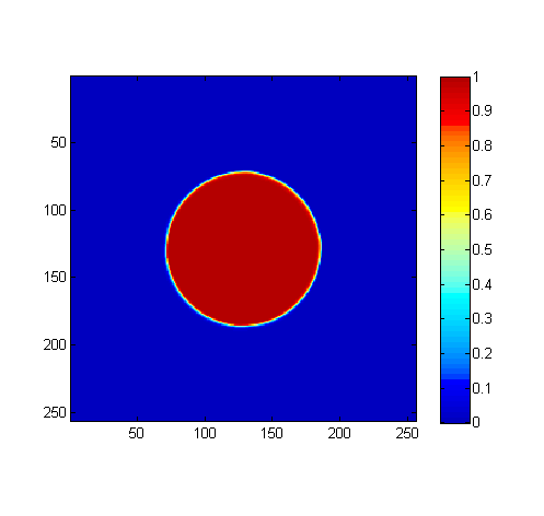
(a) Colored representation of the solution $z$.

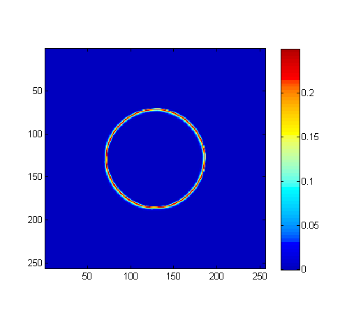
(b) Colored representation of $z(1-z)$.

Figure 9: Disk advected into a uniform vector field $\bm{u}=(1,1)$ in the domain $[-1,1]^{2}$ (periodic boundary conditions). Discrete solution at final time $t=10$, cartesian grid $256^{2}$ using the MLP+RK2 strategy.

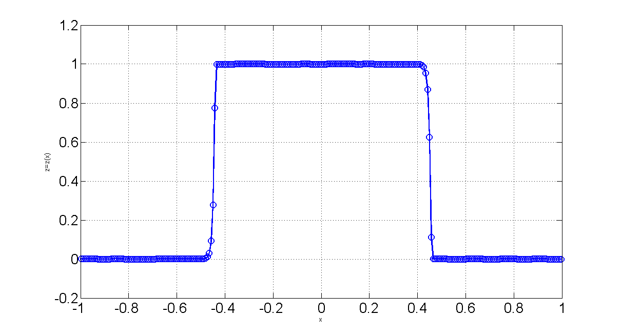
(a) Horizontal cut plane $(y=0)$.

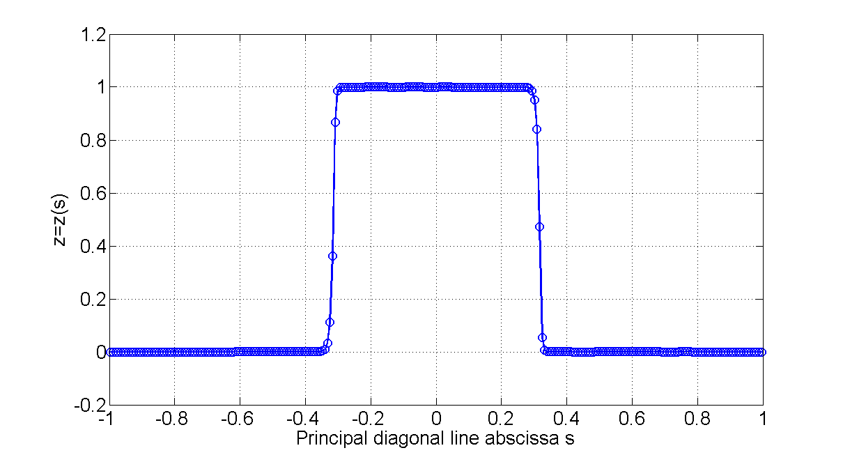
(b) principal diagonal cut plane.

Figure 10: Plots of $z$ profiles for different cut planes.

6.2 Advection of a disk into a pure rotation vector field

We have also tested the case of rigid rotation of a disk from section 2.2. This time, applying the (MLP+RK2) strategy leads to an accurate transport of the disk, free from any zigzag instabilities. The profile on an horizontal cut plane again shows sharp discontinuities after one disk revolution.

6.3 Experimental error measurements on the stationary oblique discontinuity problem

To complete the experiments, we take again the third case of steady oblique discontinuity presented in section 2.2 and perform a convergence analysis. On figure 11, we plot the discrete steady field obtained with MLP+RK2 for different grid refinement: $32\times 32$, $64\times 64$ and $512\times 512$ respectively. More interesting is the measured convergence rates shown on figure 12. We find a numerical convergence of $0.9861$ (close to 1) for the $L^{1}$-norm and $0.494$ (close to 1/2) for the $L^{2}$-norm, showing the accuracy level of the method. Remark also that the measured global conservation error convergence

$$E(h)=\left|\int_{\Omega}(z^{h}-z^{\infty})\,d\bm{x}\right|$$

is not zero exactly because of second-order errors of boundary outstream fluxes, but anyway it is second-order accurate.

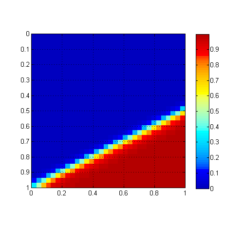
(a) Grid $32\times 32$

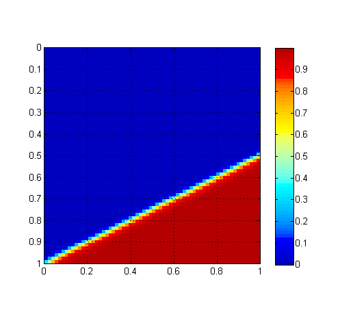
(b) Grid $64\times 64$

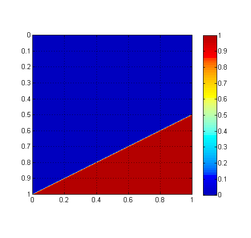
(c) Grid $512\times 512$

Figure 11: Convergence analysis on the oblique discontinuity stationary problem

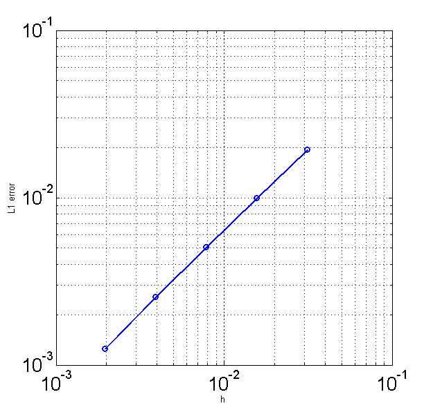
(a) Convergence analysis in $L_{1}$ norm
(log scale). Slope = 0.9861 (almost 1).

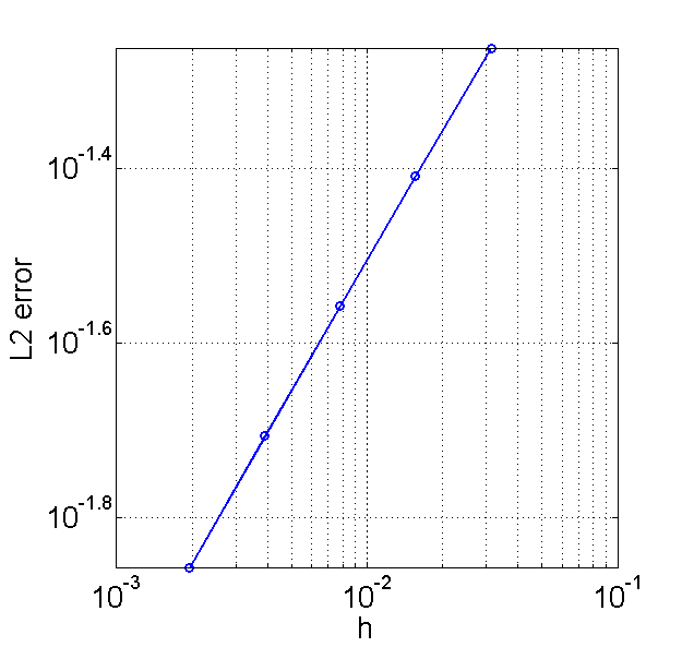
(b) Convergence analysis in $L_{2}$ norm
(log scale). Slope = 0.494 (almost $1/2$).

Figure 12: Convergence rates in $L_{1}$ and $L_{2}$ norms. Note that the convergence rate of the quantity $E(h)=\left|\int_{\Omega}(z^{h}-z^{\infty})\,d\bm{x}\right|$ is 2.

6.4 Zalesak’s disk reference case

We consider here the classical test case of rigid rotation of Zalesak’s disk in a constant rotating velocity field [41]: $\bm{u}(x,y)=(1/2-y,x-1/2)$ on the domain $\Omega=(0,1)^{2}$. The initial data $z^{0}$ is associated to a slotted circle centered at $(1/2,7/10)$ with a radius $r=1/5$, the slot depth is $3/10$ and the width is equal to $1/10$. We use a cartesian mesh composed of $512\times 512$ points. On figure 13, the $z$ field is plotted after one revolution ($t=2\pi$). One can observe the rather good accuracy of the discrete solution. Some corner effects can be observed, mainly due to the fact that the solution is not differentiable at corners, leading to discrete gradient inaccuracies. On figure 14 the $z$ profile along the line $y=7/10$ showing sharp discontinuities and the low-diffusive property using MLP.

(a) Colored representation of the solution $z$ after one revolution.

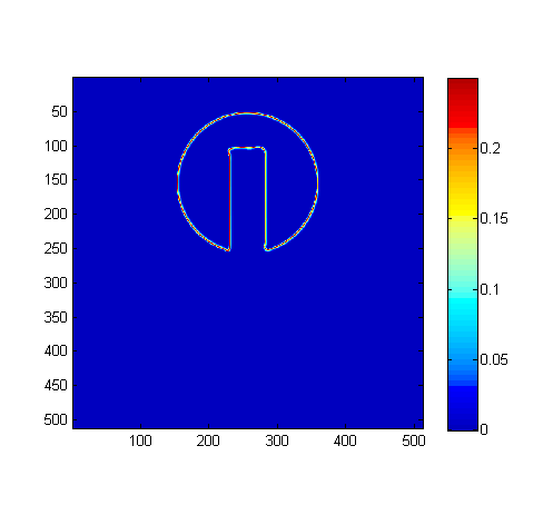
(b) Colored representation of $z(1-z)$ after one revolution.

Figure 13: Zalesak’s disk reference case, grid $512\times 512$.

Figure 14: Zalesak’s disk: $z$ profile at the cut plane $y=7/10$ after one revolution.

6.5 Reference Kothe-Rider forward-backward advection and stretching case

The reference case proposed to Rider and Kothe [32] is the deformation of a disk into a rotating and stretching velocity field. A forward-then-backward velocity field allows to come back to the initial condition (reversible process) and thus to assess the accuracy of the approach by measuring the deviation between the final time solution and the initial one. We performed two tests with two different grid levels, the first one with a grid composed of $300\times 300$ cells (figure 15) and the second one with a grid $500\times 500$ (figure 16). Using the coarsest grid, one can observe a smearing regions in the final solution, mainly to the numerical diffusion produced by the stretching process, but the initial disk shape is rather preserved. For the $500^{2}$-grid, the discrete solution at final time is very satisfactory with a preserved disk shape, showing the accuracy of the approach. The low-diffusive interface capturing process has been able to capture the stretching effect without any artefacts or instabilities.

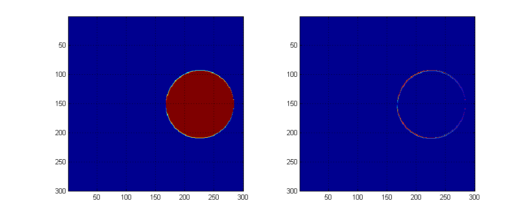
(a) At initial time $t=0$

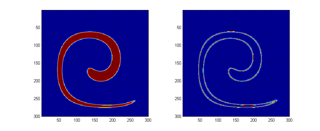
(b) At time $t=3$

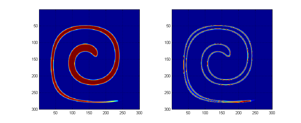
(c) At time $t=6$

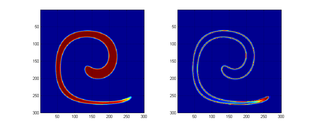
(d) At time $t=9$

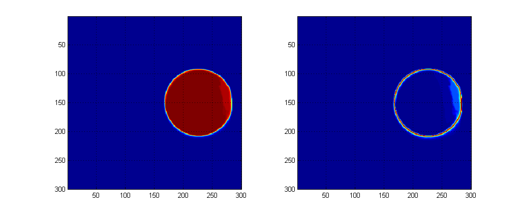
(e) At final time $t=12$

Figure 15: Validating the MLP+RK2 strategy on the Kothe-Rider advection case, cartesian mesh grid $300^{2}$.

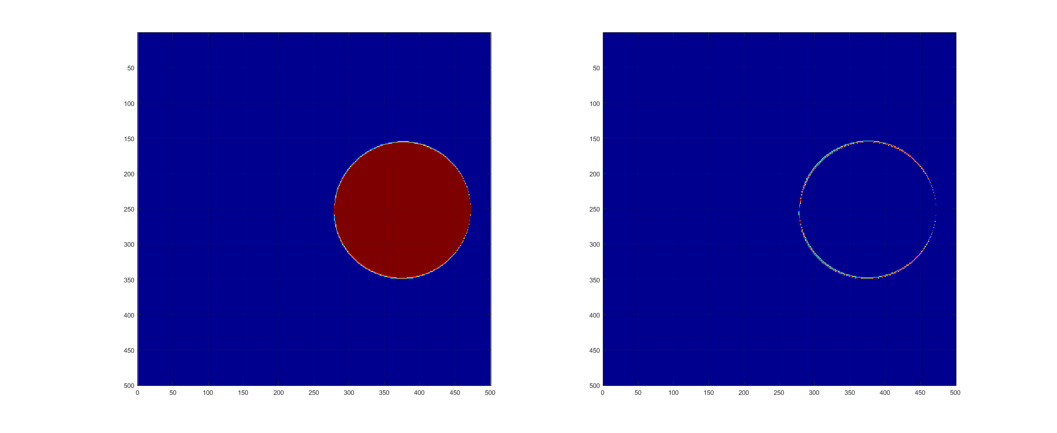
(a) At initial time $t=0$

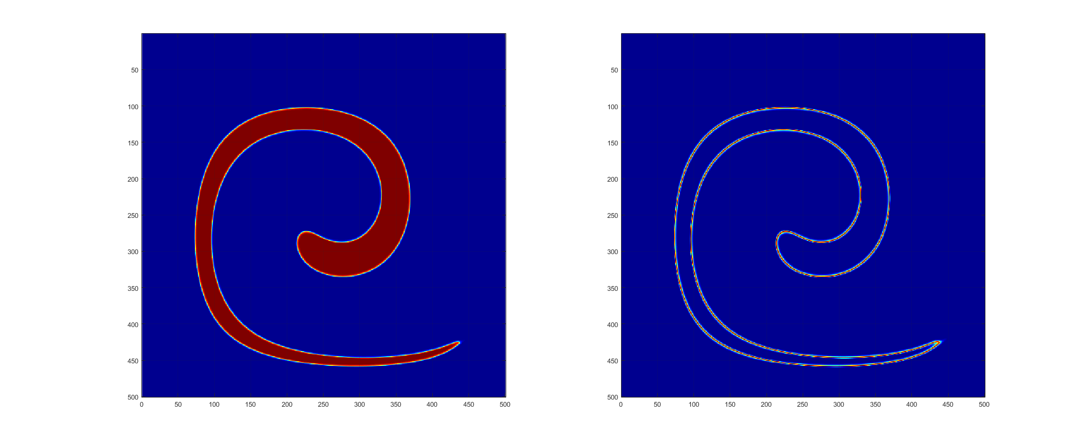
(b) At time $t=3$

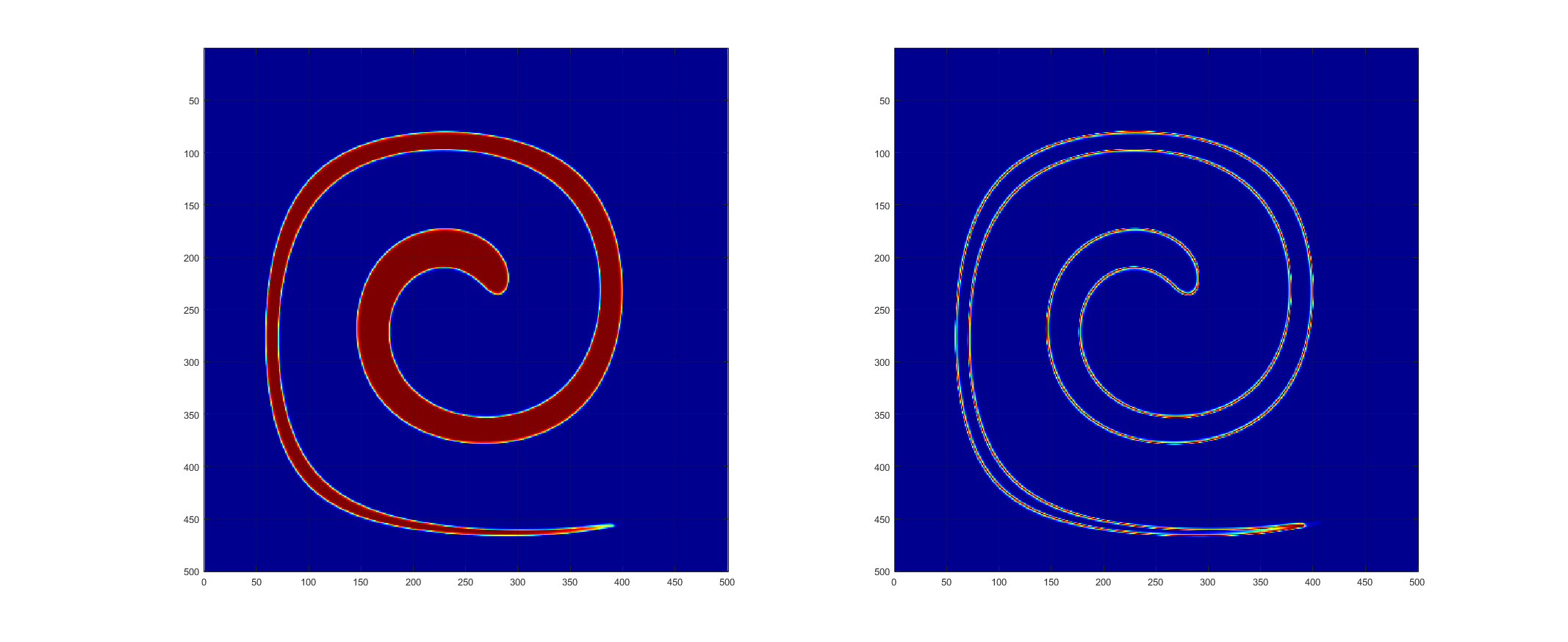
(c) At time $t=6$

(d) At time $t=9$

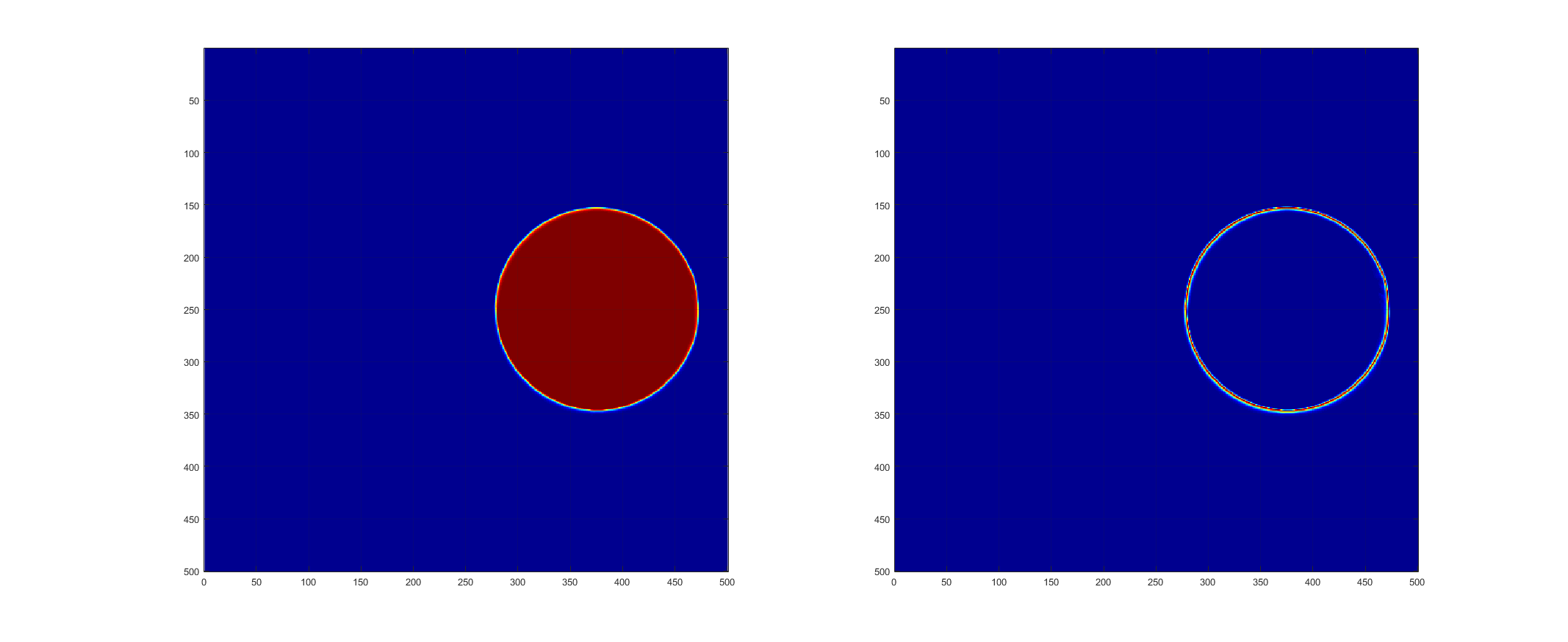
(e) At final time $t=12$

Figure 16: Validating the MLP+RK2 strategy on the Kothe-Rider advection case, cartesian mesh grid $500^{2}$.

7 Extending to compressible multimaterial flows

In this section we would like to give ideas and highlights on how the method can be extended to compressible multifluid/multimaterial hydrodynamic flows in the presence of several immiscible fluids. Even if fluids are assumed be immiscible, we use volume averaged-like balance equations because of finite volume averages that may create what we call “mixed cells” when more than one fluid in present in a cell. Of course, for the continuous problem, volume fractions should be either 0 or 1. Consider the mass, momentum and total density energy conservation equations for a system of inviscid fluids

$$\partial_{t}(\alpha_{\ell}\rho_{\ell})+\nabla\cdot(\alpha_{\ell}\rho_{\ell}\bm{u})=0,\quad\ell=1,...,N,$$

$$\partial_{t}(\rho\bm{u})+\nabla\cdot(\rho\bm{u}\otimes\bm{u})+\nabla p=0,$$

$$\partial_{t}(\rho E)+\nabla\cdot(\rho E\bm{u})+\nabla\cdot(p\bm{u})=0,$$

where $\rho_{\ell}$, $\ell=1,...,N$ denote the partial densities of each fluid, the variables $\alpha_{\ell}\in[0,1]$ are the volume fractions of each fluid, $p$ denote the pressure of the fluid (we assume local mechanical equilibrium), $\rho=\sum_{\ell=1}^{N}\alpha_{\ell}\rho_{\ell}$ is the volume-averaged density and $\rho E$ is the “mixture” total density energy, sum of both kinetic and internal density energies:

$$\rho E=\frac{1}{2}\rho|\bm{u}|^{2}+\sum_{\ell=1}^{N}\alpha_{\ell}\rho_{\ell}e_{\ell}.$$

To this system we add the volume compatibility relation

$$\sum_{\ell=1}^{N}\alpha_{\ell}=1$$

and equations of states (EOS) of each fluid, linking both density and internal energy to the fluid pressure and temperature:

$$\rho_{\ell}=\rho_{\ell}(p_{\ell},T_{\ell}),\quad\quad e_{\ell}=e_{\ell}(p_{\ell},T_{\ell}).$$

To close the system, we will here assume the simplest closure of local temperature equilibrium and local pressure equilibrium, i.e.

$$T_{1}=...=T_{N}=T,\quad\quad p_{1}=...=p_{N}=p.$$

For simplicity, we will assume here a system of perfect gases, where

$$p_{\ell}=\rho_{\ell}\frac{R}{M_{\ell}}T_{\ell},\quad e_{\ell}=c_{v;\ell}T_{\ell},$$

with $R$ the universal constant of perfect gases, $M_{\ell}$ the molar mass of fluid $\ell$, $c_{v;\ell}>0$ the (constant) specific heat at constant volume. We have also the relation

$$\gamma_{\ell}-1=\frac{c_{v;\ell}R}{M_{\ell}},$$

where $\gamma_{\ell}>1$ is the (constant) specific heat ratio so that

$$p_{\ell}=(\gamma_{\ell}-1)\rho_{\ell}e_{\ell}.$$

It is known that the resulting system of partial differential equations is hyperbolic on the admissible state space of positive densities and positive temperatures. For more general equations of state like stiffened gases and well-posedness issues, see [14] for example.

From the conservative variables $m_{\ell}:=\alpha_{\ell}\rho_{\ell}$, $\rho\bm{u}$ and $\rho E$ one can compute the primitive variables following the calculation sequence

$$\rho=\sum_{\ell=1}^{N}m_{\ell},\quad\bm{u}=\frac{\rho\bm{u}}{\rho},\quad T=\frac{\rho E-1/2\rho|\bm{u}|^{2}}{\sum_{\ell=1}^{N}c_{v;\ell}m_{\ell}},$$

$$p=\sum_{\ell=1}^{N}\alpha_{\ell}\ p=\sum_{\ell=1}^{N}(\gamma_{\ell}-1)m_{\ell}c_{v;\ell}T,$$

$$e_{\ell}=c_{v;\ell}T,$$

$$\rho_{\ell}=\frac{1}{\gamma_{\ell}-1}\frac{p}{e_{\ell}},\ \quad\alpha_{\ell}=\frac{m_{\ell}}{\rho_{\ell}},\quad\rho=\sum_{\ell=1}^{N}\alpha_{\ell}\rho_{\ell}$$

without ambiguity. Rather than volumes fraction $\alpha_{\ell}$, one could also use mass fractions $z_{\ell}$ defined by

$$z_{\ell}=\frac{\alpha_{\ell}\rho_{\ell}}{\rho}.$$

Then mass conservation equations read

$$\partial_{t}(\rho z_{\ell})+\nabla\cdot(\rho z_{\ell}\bm{u})=0.$$

Then from the continuity equation $\partial_{t}\rho+\nabla\cdot(\rho\bm{u})=0$, one can observe that the variables $z_{\ell}$ are advected according to the fluid velocity. For smooth solutions of the problem we have the equivalent transport equations

$$\partial_{t}z_{\ell}+\bm{u}\cdot\nabla z_{\ell}=0.$$

Thus we want to apply our interface capturing approach to the variables $z_{\ell}$, while guaranteeing that the numerical scheme is conservative on all the conservative variables and ensuring global numerical stability. Remark that we can pass from volume fraction variables to mass fractions by the direct and inverse formulas:

$$z_{\ell}=\frac{\alpha_{\ell}\rho_{\ell}}{\sum_{m=1}^{N}\alpha_{m}\rho_{m}},\quad\quad\alpha_{\ell}=\frac{z_{\ell}\tau_{\ell}}{\sum_{m=1}^{N}z_{m}\tau_{m}}.$$

with $\tau_{m}=(\rho_{m})^{-1}$ as specific volumes. Of course, we have again the compatibility relation on the mass fractions $\sum_{\ell=1}^{N}z_{\ell}=1$.

7.1 Lagrange+remap scheme

Our strategy of discretization follows the classical remapped Lagrange schemes made of two steps: i) first step is a full solution of the problem with a Lagrangian flow description; ii) a remap step allowing to project the quantities onto the reference (Eulerian) mesh. Let us assume that the Lagrange step, in which mass fractions are kept unchanged, is correctly solved (use for example collocated Lagrange solvers proposed by Després-Mazeran [12] or Maire et al. [25]). We rather shall focus on the remap step, seen as a convective flux step.

Rather than performing geometrical projections that involves mesh intersections, we use instead a convective flux formulation that involves material fluxes through the edges of the Eulerian mesh. If $\bm{v}$ denotes the Lagrangian velocity vector field (usually chosen as a Lagrangian velocity field $\bm{u}^{n+1/2}$ at middle time $t^{n+1/2}$ for accuracy purposes), we claim that the remapping step is nothing else but the solution of the convection system

$$\partial_{t}(\rho W)+\nabla\cdot(\rho W\bm{v})=0.$$

with the vector of variables $W=([z_{\ell}]_{\ell},\bm{u},E)$ other a time step $\Delta t^{n}$ (see De Vuyst et al. [11]). We want to design the numerical convective fluxes in order to get accuracy, stability and low-diffusivity of the mass fractions $z_{\ell}$. Remark that, because

$$\partial_{t}\rho+\nabla\cdot(\rho\bm{v})=0$$

in the remap step, actually all the variables of the $W$ vector are advected:

$$\partial_{t}W+\bm{v}\cdot\nabla W=0$$

and thus could satisfy a discrete local maximum principle in the step, providing a stability result for this step (in $L^{\infty}$ norm for example).

In order to control the mass fractions $z_{\ell}$ in $L^{\infty}$ norm, we shall follow ideas from Larrouturou [21]: considering a (semi-discrete) mass balance finite volume scheme

$$\frac{d\rho_{K}}{dt}=-\frac{1}{|K|}\sum_{A\subset\partial K}|A|\Phi_{\rho,A}$$

for a total mass flux $\Phi_{\rho,A}$ through the edge $A$, we consider partial mass balance schemes in the form

$$\frac{d(\rho z_{\ell})_{K}}{dt}=-\frac{1}{|K|}\sum_{A\subset\partial K}|A|(z_{\ell})_{A}\,\Phi_{\rho,A}$$

with a value of mass fraction $(z_{\ell})_{A}$ at the edge $A$, to define. Proceeding like that, one can check that we have

$$\frac{d(z_{\ell})_{K}}{dt}=-\frac{1}{|K|}\sum_{A\subset\partial K}|A|\left[(z_{\ell})_{A}-(z_{\ell})_{K}\right]\,\frac{\Phi_{\rho,A}}{\rho_{K}}.$$

Under CFL-like conditions of the type

$$\frac{\Delta t\,|A|}{|K|}\,\frac{|\Phi_{\rho,A}|}{\rho_{K}}\leq 1\quad\quad\forall A\in\partial K,\ \forall K,$$

it is not difficult to derive explicit first-order schemes that fulfill a local discrete maximum principle. For that, it is natural to introduce upwind edge values $(z_{\ell})_{A}$ according to the sign of the mass flux $\Phi_{\rho,A}$. Upwind values will be then denoted $(z_{\ell})_{A}^{upw}$ in the sequel.

Contact discontinuities and pressure oscillations.

As emphasized by many authors, conservative schemes may lead to important concentrated pressure oscillations through contact discontinuities (see [34] for instance) for multifluid flows. The reason behind that is that there are incompatibilities between the numerical viscous profile of total density or partial densities and profiles of mass fractions.

To fix this problem, is it important to compute edge quantities that are compatible with the (current local) pressure. The leading algorithm is the following one :

1. For each cell $K$, compute the pressure variable $p_{K}$ and temperature variable $T_{K}$;

2. Compute the associated partial densities $(\rho_{\ell})_{K}=\rho_{\ell}(p_{K},T_{K})$;

3. Compute the edge mass fractions $(z_{\ell})_{A}$ from the MLP algorithm presented in a previous section;

4. Then deduce from the $(z_{\ell})_{A}$ and $(\rho_{\ell})_{K}$ the volume fractions :

   $$(\alpha_{\ell})_{A}=\frac{(z_{\ell})_{A}(\tau_{\ell})_{K}}{\sum_{m=1}^{N}(z_{m})_{A}(\tau_{m})_{K}};$$

5. Compute a mean edge density $\rho_{A}$ as

   $$\rho_{A}=\sum_{\ell=1}^{N}(\alpha_{\ell})_{A}(\rho_{\ell})_{K}$$

6. For each edge, compute the upwind edge density $\rho_{A}^{upw}$ from the extrapolated values $\rho_{A}$ and deduce a mass flux

   $$\Phi_{\rho,A}=\rho_{A}^{upw}\,(\bm{v}_{A}\cdot\nu_{A}).$$

7. For each edge, deduce the upwind edge volume fractions $(z_{\ell})_{A}^{upw}$ according to the sign of the mass flux $\Phi_{\rho,A}$;

8. Integrate the semi-discrete scheme

   $$\frac{d(\alpha_{\ell}\rho_{\ell})_{K}}{dt}=-\frac{1}{|K|}\sum_{A\subset\partial K}|A|(z_{\ell})_{A}^{upw}\,\Phi_{\rho,A}$$

   over a time step $\Delta t$.

Of course this algorithm can be easily extended to second-order accuracy in space. For that, consider MUSCL reconstructions on the thermodynamic variables $p$ and $T$. Then for each cell $K$ we have to compute extrapolated values of pressure and temperature $p_{A}$ and $T_{A}$ respectively at edge $A$, then compute partial densities $(\rho_{\ell})_{A}$ as

$$(\rho_{\ell})_{A}=\rho_{\ell}(p_{A},T_{A}),$$

and edge volume fractions

$$(\alpha_{\ell})_{A}=\frac{(z_{\ell})_{A}(\tau_{\ell})_{A}}{\sum_{m=1}^{N}(z_{m})_{A}(\tau_{m})_{A}},$$

then complete by the above algorithm to finish.

Gradients compatibility.

For more than two fluids, linear reconstructions must pay attention to the mass compatibility invariant

$$\sum_{\ell=1}^{N}z_{\ell}=1.$$

The MLP reconstruction requires both prediction and limitation of each gradient per species $\ell$. For a gradient reconstruction on the mass fraction $z_{\ell}$ par cell $K$, i.e.

$$\mathscr{I}^{h}z_{\ell}(\bm{x})=(z_{\ell})_{K}+(\phi_{\ell})_{K}(\nabla^{h}z_{\ell})_{K}\cdot(\bm{x}-\bm{x}_{K}),$$

because we want for any $\bm{x}$ in $K$ to have

$$\sum_{\ell=1}^{n}\mathscr{I}^{h}z_{\ell}(\bm{x})=1,$$

we get the expected compatibility formula on the limited gradients

$$\sum_{\ell=1}^{N}(\phi_{\ell})_{K}(\nabla^{h}z_{\ell})_{K}=\bm{0}.$$ (8)

As a first remark, if the apply the gradient prediction formula (7) for each fluid $\ell$, by linearity of the formula we clearly have

$$\sum_{\ell=1}^{N}(\nabla^{h}z_{\ell})_{K}=\bm{0}.$$

The difficulty here is once again due to the linear procedure of limitation which may violate the identity (8). We propose the following algorithm: first, apply the MLP, as explained in previous sections, for each fluid $\ell$. We get an estimator of limiting factor for each $\ell$, here denoted by $\widehat{(\phi_{\ell})}_{K}$, $\widehat{(\phi_{\ell})}_{K}\geq 0$.

In a second step, we have to find a procedure to more limit these factors in order to satisfy the identity (8). This can be done for example by the use of a linear-quadratic (LQ) optimization problem

$$\max_{(\phi_{1},\phi_{2},...,\phi_{N})}\quad\frac{1}{2}\sum_{\ell=1}^{N}\phi_{\ell}^{2}$$ (9)

subject to the bound inequality constraints

$$0\leq\phi_{\ell}\leq\widehat{(\phi_{\ell})}_{K},\quad\ell\in\{1,...,N\}$$

and compatibility linear equality constraints

$$\sum_{\ell=1}^{N}\phi_{\ell}\,(\nabla^{h}z_{\ell})_{K}=\bm{0}.$$

This optimization problem can be easily solved by standard duality theory [3]. We will do not detail the resulting algorithm. The construction may be a little more diffusive because of the double limitation process, but let us emphasize that areas with more than two materials are generally sparse, limited to singular topology elements like triple-points for example.

7.2 Numerical evaluation on the reference “triple-point” test case

The resulting hydrodynamic solver is tested on the reference “triple point” test case, found e.g. in Loubère et al. [24]. This problem is a three-state two-material 2D Riemann problem in a rectangular vessel. The simulation domain is $\Omega=(0,7)\times(0,3)$ as described in figure 17. The domain is splitted up into three regions $\Omega_{i}$, $i=1,2,3$ filled with two perfect gases leading to a two-material problem. Perfect gas equations of state are used with $\gamma_{1}=\gamma_{3}=1.5$ and $\gamma_{2}=1.4$. Due to the density differences, two shocks in subdomains $\Omega_{2}$ and $\Omega_{3}$ propagate with different speeds. This create a shear along the initial contact discontinuity and the formation of a vorticity. Capturing the vorticity is of course the difficult part to compute. We use a rather fine mesh made of $2048\times 878$ points (about 1.8M cells).

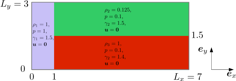
Figure 17: Geometry and initial configuration for the reference triple-point case.

On figure 18, the numerical solution at final time $T_{f}=3.3530$. We also provide on figure 6 a zoom of the vorticity zone to show the accuracy of the interface captures in this area.

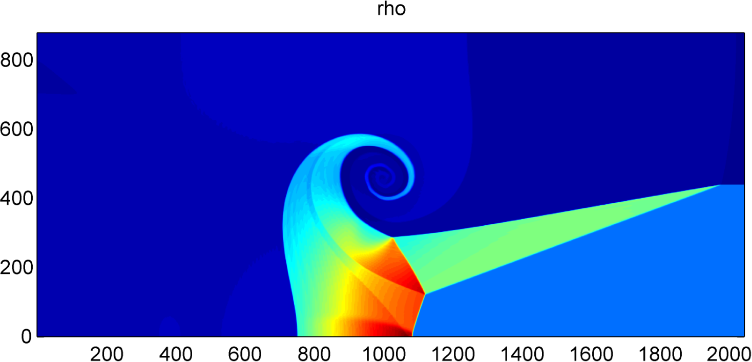
(a) Density field

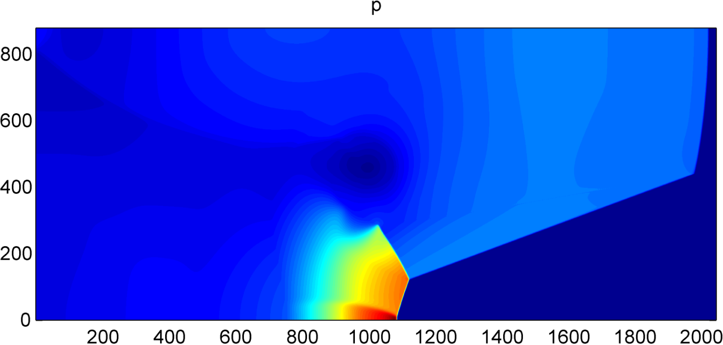
(b) Pressure field

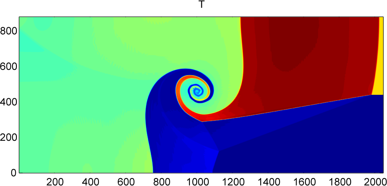
(c) Temperature field

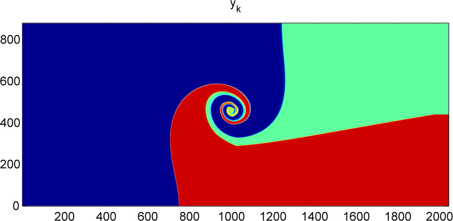
(d) Colored representation of material indicators

Figure 18: Results on the multimaterial “triple point” case (perfect gases) using a collocated Lagrange+remap solver + low-diffusive interface capturing advection scheme, mesh 2048x878. Final time is $T_{f}=3.3530$.

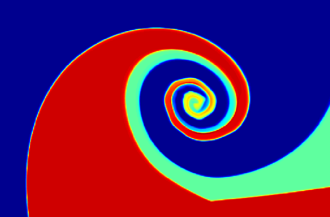
Figure 19: Triple point, zoom-in of the vortex region at final time, mesh 2048x878.

8 Concluding remarks and perspectives

In this paper, topics on accuracy, stability and artefact-free interface capturing methods have been discussed and analyzed. On this subject of high interest for the whole Hydrodynamics community, of course one can already find important literature and contributions. We have tried to shed a new light and bring our understanding of this tricky subject. Artefacts commonly encountered with interface capturing schemes (including strange attractor shapes like octagons on cartesian grids, privileged directions artefacts, zigzag interface instabilities) are mainly due to a misbalance between too much antidiffusion and expected accuracy, but also because of important errors of gradient direction estimation. In particular direction-by-direction compressive slope limiters (superbee, ultrabee, limited downwind, …) are too compressive in some directions and do not take into account the direction normal to the interface which has to be evaluated accurately as demonstrated in this paper. For this purpose, a multidimensional limiting process (MLP) strategy appears to be a good candidate that first evaluate the gradient direction without any nonlinear limitation, and then limit the gradient intensity in order to get local extremum diminishing (LED) properties. Numerical evidence also shows that a first-order explicit Euler scheme creates linear instabilities that evolve toward spurious zigzag-shaped interface modes when the numerical advective flux does not include the compensating Lax-Wendroff term. Rather than including a Lax-Wendroff diffusive flux, we rather use a Runge-Kutta RK2 time integrator that allows to kill zigzag instabilities. The whole MLP+RK2 strategy provide a stable and accurate diffuse interface capturing approach with an acceptable discrete interface compactness. Although it is not at the aim on paper, we wanted to have a first result of extension to compressible multimaterial hydrodynamics to show both generalisation and flexibility of the method and have a first idea of the competitiveness of the method, especially compared to interface reconstruction algorithms. We believe that this approach is promising in terms of accuracy and computing performance (pure SIMD algorithms with natural parallelization on multicore/manycore architectures). We also intend to extend and evaluate the approach on unstructured meshes.

References

- [1] H.T. Ahn and M. Shashkov, Multimaterial interface reconstruction on generalized polyhedral meshes, Journal of Comp. Phys., 226, 2096–2132 (2007).
- [2] O. Bokanowski and H. Zidani, Anti-Dissipative Schemes for Advection and Application to Hamilton-Jacobi-Bellmann Equations, Journal of Scientific Computing, 40(1), 1–33 (2007).
- [3] J.-F. Bonnans, J.C. Gilbert, C. Lemaréchal and C.A. Sagastizábal, Numerical optimization, Theoretical and practical aspects, Springer Universitext (2006).
- [4] J.Ph. Braeunig, J.M. Ghidaglia and R. Loubère, A totally Eulerian Finite Volume solver for multi-material fluid flows : Enhanced Natural Interface Positioning (ENIP), European Journal of Mechanics - B/Fluids Volume 31, 1–11 (2012).
- [5] J. Breil, T. Harribey, P.-H. Maire, M. Shashkov, A multi-material ReALE method with MOF interface reconstruction, Computers and Fluids, 83, 115–125 (2013).
- [6] A. Caboussat, M.M. Francois, R. Glowinski, D.B. Kothe, J.M. Sicilian, A numerical method for interface reconstruction of triple points within a volume tracking algoirithm, Math. and Comp. Modelling, Vol 48(11-12), 1957–1971 (2008).
- [7] A. Bernard-Champmartin and F. De Vuyst, A low diffusive Lagrange-remap scheme for the simulation of violent air-water free-surface flows, Journal of Computational Physics, vol. 274, 19–49 (2014).
- [8] B. Després and F. Lagoutière, Contact discontinuity capturing schemes for linear advection and compressible gas dynamics, J. Sci. Comp., 16(4), 479–524 (2001).
- [9] B. Després and F. Lagoutière, Genuinely multi-dimensional non-dissipative finite-volume scheme for transport, Int. J. Appl. Math. Comput. Sci., 17(3), 321–328 (2007).
- [10] B. Després, F. Lagoutière, E. Labourasse and I. Marmajou, An antidissipative transport scheme on unstructured meshes for multicomponent flows, IJFV, 30–65 (2010).
- [11] F. De Vuyst, T. Gasc, R. Motte, M. Peybernes and R. Poncet, Lagrange-flux schemes: reformulating second-order accurate Lagrange-remap schemes for better node-based HPC performance, submitted to OGST (2016).
- [12] B. Després and C. Mazeran, Lagrangian gas dynamics in two dimensions and Lagrangian systems, Arch. Rational Mech. Anal., 178, 327–372 (2005).
- [13] V. Faucher and S. Kokh, Extended Vofire algorithm for fast transient fluid-structure dynamics with liquid-gas flows and interfaces, J. Fluids and structures, 39, pp. 25 (2013).
- [14] T. Flåtten, A. Morin and S.T. Munkejord, On solutions to equilibrium problems for systems of stiffened gases, SIAM J. Appl. Math., 71(1), 41–67 (2011).
- [15] T. Gasc, F. De Vuyst, Suitable formulations of Lagrange Remap Finite Volume schemes for manycore / GPU architectures, Finite Volumes for Complex Applications VII, Springer Proc. in Math. & Stat., vol. 78, 607–616 (2014).
- [16] E. Godlewski and P.A. Raviart, Numerical approximation of hyperbolic systems of conservation laws, Applied Mathematical sciences, Springer (1996).
- [17] R.N. Hill and M. Shashkov, The symmetric moment-of-fluid interface reconstruction algorithm, J. Comp. fluids, 249, 180–184 (2013).
- [18] A.I. Khrabry, E.M. Smirnov and D.K. Zaytsev, Solving the convective transport equation with several high-resolution finite volume schemes: test computations, in Computational Fluid Dynamics 2010, Proc. of the ICCFD6, A. Kuzmin Ed., 535–540 (2011).
- [19] D. Kuzmin and S. Turek, High-resolution FEM-TVD schemes based on a fully multidimensional flux limiter, J. Comput. Phys., 198(1), 131–158 (2004).
- [20] D. Kuzmin, On the design of general-purpose flux limiters for implicit FEM with a consistent mass matrix. I. Scalar convection”, Journal of Computational Physics 219 (2), 513–-531 (2006).
- [21] B. Larrouturou, How to preserve the mass fraction positive when computing compressible multi-component flows, J. Comp. Phys., 95(1), 59–84 (1991).
- [22] B.P. Leonard, The ULTIMATE conservative difference scheme applied to unsteady one dimensional advection, Comput. Meth. Appl. Mech. Eng., 88, 17–74 (1991).
- [23] R. Leveque, High-resolution conservative algorithms for advection in incompressible flow, SIAM J. Num. Anal, 33(2), 627–665 (1996).
- [24] R. Loubère, P.-H. Maire, M. Shashkov, J. Breil and S. Galera, ReALE: A reconnection-based arbitrary-Lagrangian-Eulerian method, J. Comp. Phys., 229, 4724–4761 (2010).
- [25] R. Loubère, P.-H. Maire and P. Váchal, Staggered Lagrangian discretization based on cell-centered Riemann solver and associated hydrodynamics scheme, Comm. in Comp. Phys., 10(4), 940–978 (2011).
- [26] A. Michel, Q.H. Tran and G. Favennec, A genuinely one-dimensional upwind scheme with accuracy enhancement for multidimensional advection problems, ECMOR XII - 12th European Conference on the Mathematics of Oil Recovery (2010).
- [27] S. Muzaferija and M. Perić, Computation of free surface flows using interface-tracking and interface-capturing methods, in O. Mahrenholtz, M. Markiewicz (eds.), Nonlinear water wave interaction, chap. 2, 59–100, WIT Press, Southampton (1999).
- [28] S. Osher and R.P. Fedkiw, Level set methods: an overview and some recent results. J. Comput. Phys., 169(2), 463–502 (2001)/
- [29] J.S. Park and C. Kim, Multi-dimensional Limiting Process for Discontinuous Galerkin Methods on Unstructured Grids, chapter in Computational Fluid Dynamics 2010, Springer, 179–184 (2011).
- [30] R. Poncet, M. Peybernes, T. Gasc and F. De Vuyst, Performance modeling of a compressible hydrodynamics solver on multicore CPUs, Proc. of the Conference PARCO 2015, Edinburgh, to appear (2015).
- [31] L. Qian, D.M. Causon, C.G. Mingham and D.M. Ingram, A free-surface capturing method for two fluid flows with moving bodies, Proc. of the Royal Soc. of London A: Mathematical, Physical and Eng. Sci., 462(2065), 21–42 (2006).
- [32] A.J. Rider and D.B. Kothe, Reconstructing volume tracking, J. Comput. Phys., 141(2), 112–152 (1998).
- [33] P.L. Roe, Some contributions to the modeling of discontinuous flows, in Proc. of the SIAM/AMS Seminar, San Diego, 1983.
- [34] R. Saurel and R. Abgrall, A multiphase Godunov method for compressible multifluid and multiphase flows, J. Comp. Phys., 150, 425–467 (1999).
- [35] P.K. Sweby, High resolution schemes using flux-limiters for hyperbolic conservation laws”, SIAM J. Num. Anal. 21 (5), 995-–1011 (1984).
- [36] J. Thuburn, Multidimensional flux-limited advection schemes, J. Comp. Phys., 123(1), 74–83 (1996).
- [37] E.F. Toro, Riemann solvers and numerical methods for fluid dynamics, 3rd Edition, Springer (2010).
- [38] O. Ubbink and R.I. Issa, A method for capturing sharp fluid interfaces on arbitrary meshes, J. Comp. Phys., 153(1), 26–50 (1999).
- [39] T. Waclawczyk, T. Koronowicz, Remarks on prediction on wave drag using VOF method with interface capturing approach, Arch. Civ. Mech. Eng., 8(1), 5–14 (2008).
- [40] S.H. Yoon, C. Kim and K.H. Kim, Multi-dimensional Limiting Process for Two- and Three-dimensional Flow Physics Analyses, chapter in Computational Fluid Dynamics 2006, Springer, 185–190 (2009).
- [41] S. Zalesak, Fully multidimensional flux-corrected transport algorithms for fluids, J. Comput. Phys. 31, 335-–362 (1979).
- [42] D. Zhang, C. Jiang, D. Liang, Z. Chen, Y. Yan and Y. Shi, A refined volume-of-fluid algorithm for capturing sharp fluid interfaces on arbitrary meshes, J. Comp. Phys., 274, 709–736 (2014).