Abstract

Bayesian optimization has become a successful tool for hyperparameter optimization of machine learning algorithms, such as support vector machines or deep neural networks. Despite its success, for large datasets, training and validating a single configuration often takes hours, days, or even weeks, which limits the achievable performance. To accelerate hyperparameter optimization, we propose a generative model for the validation error as a function of training set size, which is learned during the optimization process and allows exploration of preliminary configurations on small subsets, by extrapolating to the full dataset. We construct a Bayesian optimization procedure, dubbed Fabolas, which models loss and training time as a function of dataset size and automatically trades off high information gain about the global optimum against computational cost. Experiments optimizing support vector machines and deep neural networks show that Fabolas often finds high-quality solutions 10 to 100 times faster than other state-of-the-art Bayesian optimization methods or the recently proposed bandit strategy Hyperband.

1 Introduction

The performance of many machine learning algorithms hinges on certain hyperparameters. For example, the prediction error of non-linear support vector machines depends on regularization and kernel hyperparameters $C$ and $\gamma$; and modern neural networks are sensitive to a wide range of hyperparameters, including learning rates, momentum terms, number of units per layer, dropout rates, weight decay, etc. (Montavon et al., 2012). The poor scaling of naïve methods like grid search with dimensionality has driven interest in more sophisticated hyperparameter optimization methods over the past years (Bergstra et al., 2011; Hutter et al., 2011; Bergstra and Bengio, 2012; Snoek et al., 2012; Bardenet et al., 2013; Bergstra et al., 2013; Swersky et al., 2013, 2014; Snoek et al., ; Snoek et al., 2015). Bayesian optimization has emerged as an efficient framework, achieving impressive successes. For example, in several studies, it found better instantiations of convolutional network hyperparameters than domain experts, repeatedly improving the top score on the CIFAR-10 (Krizhevsky, 2009) benchmark without data augmentation (Snoek et al., 2012; Domhan et al., 2015; Snoek et al., 2015).

In the traditional setting of Bayesian hyperparameter optimization, the loss of a machine learning algorithm with hyperparameters ${\bm{x}}\in\mathbb{X}$ is treated as the “black-box” problem of finding $\operatornamewithlimits{arg\,min}_{{\bm{x}}\in\mathbb{X}}f({\bm{x}})$, where the only mode of interaction with the objective $f$ is to evaluate it for inputs ${\bm{x}}\in\mathbb{X}$. If individual evaluations of $f$ on the entire dataset require days or weeks, only very few evaluations are possible, limiting the quality of the best found value. Human experts instead often study performance on subsets of the data first, to become familiar with its characteristics before gradually increasing the subset size (Bottou, 2012; Montavon et al., 2012). This approach can still outperform contemporary Bayesian optimization methods.

Motivated by the experts’ strategy, here we leverage dataset size as an additional degree of freedom enriching the representation of the optimization problem. We treat the size of a randomly subsampled dataset $N_{sub}$ as an additional input to the blackbox function, and allow the optimizer to actively choose it at each function evaluation. This allows Bayesian optimization to mimic and improve upon human experts when exploring the hyperparameter space. In the end, $N_{sub}$ is not a hyperparameter itself, but the goal remains a good performance on the full dataset, i.e. $N_{sub}=N$.

Hyperparameter optimization for large datasets has been explored by other authors before. Our approach is similar to Multi-Task Bayesian optimization by Swersky et al. (2013), where knowledge is transferred between a finite number of correlated tasks. If these tasks represent manually-chosen subset-sizes, this method also tries to find the best configuration for the full dataset by evaluating smaller, cheaper subsets. However, the discrete nature of tasks in that approach requires evaluations on the entire dataset to learn the necessary correlations. Instead, our approach exploits the regularity of performance across dataset size, enabling generalization to the full dataset without evaluating it directly.

Other approaches for hyperparameter optimization on large datasets include work by Nickson et al. (2014), who estimated a configuration’s performance on a large dataset by evaluating several training runs on small, random subsets of fixed, manually-chosen sizes. Krueger et al. (2015) showed that, in practical applications, small subsets can suffice to estimate a configuration’s quality, and proposed a cross-validation scheme that sequentially tests a fixed set of configurations on a growing subset of the data, discarding poorly-performing configurations early.

In parallel work, Li et al. (2017) proposed a multi-arm bandit strategy, called Hyperband, which dynamically allocates more and more resources to randomly sampled configurations based on their performance on subsets of the data. Hyperband assures that only well-performing configurations are trained on the full dataset while discarding bad ones early. Despite its simplicity, in their experiments the method was able to outperform well-established Bayesian optimization algorithms.

In §2, we review Bayesian optimization, in particular the Entropy Search algorithm and the related method of Multi-Task Bayesian optimization. In §3, we introduce our new Bayesian optimization method Fabolas for hyperparameter optimization on large datasets. In each iteration, Fabolas chooses the configuration $x$ and dataset size $N_{sub}$ predicted to yield most information about the loss-minimizing configuration on the full dataset per unit time spent. In §4, a broad range of experiments with support vector machines and various deep neural networks show Fabolas often identifies good hyperparameter settings 10 to 100 times faster than state-of-the-art Bayesian optimization methods acting on the full dataset as well as Hyperband.

2 Bayesian optimization

Given a black-box function $f:\mathbb{X}\rightarrow\mathbb{R}$, Bayesian optimization aims to find an input ${\bm{x}}_{\star}\in\operatornamewithlimits{arg\,min}_{{\bm{x}}\in\mathbb{X}}f({\bm{x}})$ that globally minimizes $f$. It requires a prior $p(f)$ over the function and an acquisition function $a_{p(f)}:\mathbb{X}\rightarrow\mathbb{R}$ quantifying the utility of an evaluation at any ${\bm{x}}$. With these ingredients, the following three steps are iterated (Brochu et al., 2010): (1) find the most promising ${\bm{x}}_{n+1}\in\operatornamewithlimits{arg\,max}{a_{p}({\bm{x}})}$ by numerical optimization; (2) evaluate the expensive and often noisy function $y_{n+1}\sim f({\bm{x}}_{n+1})+\mathcal{N}(0,\sigma^{2})$ and add the resulting data point $({\bm{x}}_{n+1},y_{n+1})$ to the set of observations $\mathcal{D}_{n}=({\bm{x}}_{j},y_{j})_{j=1...n}$; and (3) update $p(f\mid\mathcal{D}_{n+1})$ and $a_{p(f\mid\mathcal{D}_{n+1})}$. Typically, evaluations of the acquisition function $a$ are cheap compared to evaluations of $f$ such that the optimization effort is negligible.

2.1 Gaussian Processes

Gaussian processes (GP) are a prominent choice for $p(f)$, thanks to their descriptive power and analytic tractability (e.g. Rasmussen and Williams, 2006). Formally, a GP is a collection of random variables, such that every finite subset of them follows a multivariate normal distribution. A GP is identified by a mean function $m$ (often set to $m({\bm{x}})=0\;\forall{\bm{x}}\in\mathbb{X}$), and a positive definite covariance function (kernel) $k$. Given observations $\mathcal{D}_{n}=({\bm{x}}_{j},y_{j})_{j=1...n}=(\boldsymbol{X},{\bm{y}})$ with joint Gaussian likelihood $p({\bm{y}}\mid\boldsymbol{X},f(\boldsymbol{X}))$, the posterior $p(f|\mathcal{D}_{n})$ follows another GP, with mean and covariance functions of tractable, analytic form.

The covariance function determines how observations influence the prediction. For the hyperparameters we wish to optimize, we adopt the Matérn $\nicefrac{{5}}{{2}}$ kernel (Matérn, 1960), in its Automatic Relevance Determination form (MacKay and Neal, 1994). This stationary, twice-differentiable model constitutes a relatively standard choice in the Bayesian optimization literature. In contrast to the Gaussian kernel popular elsewhere, it makes less restrictive smoothness assumptions, which can be helpful in the optimization setting (Snoek et al., 2012):

$$\begin{split}k_{\nicefrac{{5}}{{2}}}({\bm{x}},{\bm{x}}^{\prime})&=\theta\left(1+\sqrt{5}d_{\bm{\lambda}}({\bm{x}},{\bm{x}}^{\prime})\right.\\ &\left.+\nicefrac{{5}}{{3}}d^{2}_{\bm{\lambda}}({\bm{x}},{\bm{x}}^{\prime})\right)e^{-\sqrt{5}d_{\bm{\lambda}}({\bm{x}},{\bm{x}}^{\prime})}.\end{split}$$ (1)

Here, $\theta$ and ${\bm{\lambda}}$ are free parameters—hyperparameters of the GP surrogate model—and $d_{\bm{\lambda}}({\bm{x}},{\bm{x}}^{\prime})=({\bm{x}}-{\bm{x}}^{\prime})^{\textrm{{\sf{T}}}}\operatorname{diag}({\bm{\lambda}})({\bm{x}}-{\bm{x}}^{\prime})$ is the Mahalanobis distance. For the dataset size dependent performance and cost, we construct a custom kernel in 3.1. An additional hyperparameter of the GP model is a overall noise covariance needed to handle noisy observations. For clarity: These GP hyperparameters are internal hyperparameters of the Bayesian optimizer, as opposed to those of the target machine learning algorithm to be tuned. Section 3.4 shows how we handle them.

2.2 Acquisition functions

The role of the acquisition function is to trade off exploration vs. exploitation. Popular choices include Expected Improvement (EI) (Mockus et al., 1978), Upper Confidence Bound (UCB) (Srinivas et al., 2010), Entropy Search (ES) (Hennig and Schuler, 2012), and Predictive Entropy Search (PES) (Hernández-Lobato et al., 2014). In our experiments, we will use EI and ES.

We found EI to perform robustly in most applications, providing a solid baseline; it is defined as

$$a_{\text{EI}}({\bm{x}}|\mathcal{D}_{n}) =\mathbb{E}_{p}[\max(f_{\text{min}}-f({\bm{x}}),0)]\,.$$ (2)

where $f_{\text{min}}$ is the best function value known (also called the incumbent). This expected drop over the best known value is high for points predicted to have small mean and/or large variance.

ES is a more recent acquisition function that selects evaluation points based on the predicted information gain about the optimum, rather than aiming to evaluate near the optimum. At the heart of ES lies the probability distribution $p_{\min}({\bm{x}}\mid\mathcal{D}):=p({\bm{x}}\in\operatornamewithlimits{arg\,min}_{{\bm{x}}^{\prime}\in\mathbb{X}}f({\bm{x}}^{\prime})\mid\mathcal{D})$, the belief about the function’s minimum given the prior on $f$ and observations $\mathcal{D}$. The information gain at ${\bm{x}}$ is then measured by the expected Kullback-Leibler divergence (relative entropy) between $p_{\min}(\cdot\mid\mathcal{D}\cup\{({\bm{x}},y)\})$ and the uniform distribution $u({\bm{x}})$, with expectations taken over the measurement $y$ to be obtained at ${\bm{x}}$:

$$\begin{split}a_{\text{ES}}({\bm{x}}):&=\mathbb{E}_{p(y\mid{\bm{x}},\mathcal{D})}\left[\int p_{\min}({\bm{x}}^{\prime}\mid\mathcal{D}\cup\{({\bm{x}},y)\})\right.\\ &\left.\cdot\log\frac{p_{\min}({\bm{x}}^{\prime}\mid\mathcal{D}\cup\{({\bm{x}},y)\})}{u({\bm{x}}^{\prime})}\ \mathrm{d}{\bm{x}}^{\prime}\right].\end{split}$$ (3)

The primary numerical challenge in this framework is the computation of $p_{\min}(\cdot\mid\mathcal{D}\cup\{({\bm{x}},y)\})$ and the integral above. Due to the intractability, several approximations have to be made. We refer to Hennig and Schuler (2012) for details, as well as to the supplemental material (Section A), where we also provide pseudocode for our implementation. Despite the conceptual and computational complexity of ES, it offers a well-defined concept for information gained from function evaluations, which can be meaningfully traded off against other quantities, such as the evaluations’ cost.

PES refers to the same acquisition function, but uses different approximations to compute it. In Section 3.4 we describe why, for our application, ES was the more direct choice.

2.3 Multi-Task Bayesian optimization

The Multi-Task Bayesian optimization (MTBO) method of Swersky et al. (2013) refers to a general framework for optimizing in the presents of different, but correlated tasks. Given a set of such tasks $\mathbb{T}=\{1,\ldots,T\}$, the objective function $f:\mathbb{X}\times\mathbb{T}\rightarrow\mathbb{R}$ corresponds to evaluating a given ${\bm{x}}\in\mathbb{X}$ on one of the tasks $t\in\mathbb{T}$. The relation between points in $\mathbb{X}\times\mathbb{T}$ is modeled via a GP using a product kernel:

$$k_{\text{MT}}(({\bm{x}},t),({\bm{x}}^{\prime},t^{\prime}))=k_{T}(t,t^{\prime})\cdot k_{\nicefrac{{5}}{{2}}}({\bm{x}},{\bm{x}}^{\prime})\,.$$ (4)

The kernel $k_{T}$ is represented implicitly by the Cholesky decomposition of $k(\mathbb{T},\mathbb{T})$ whose entries are sampled via MCMC together with the other hyperparameters of the GP. By considering the distribution over the optimum on the target task $t_{*}\in\mathbb{T}$, $p_{\min}^{t_{*}}({\bm{x}}\mid\mathcal{D}):=p({\bm{x}}\in\operatornamewithlimits{arg\,min}_{{\bm{x}}^{\prime}\in\mathbb{X}}f({\bm{x}}^{\prime},t=t_{*})\mid\mathcal{D})$, and computing any information w.r.t. it, Swersky et al. (2013) use the information gain per unit cost as their acquisition function:

$$a_{\text{MT}}({\bm{x}},t): =\frac{1}{c({\bm{x}},t)}\mathbb{E}_{p(y\mid{\bm{x}},t,\mathcal{D})}\left[\int p_{\min}^{t_{*}}({\bm{x}}^{\prime}\mid\mathcal{D}^{\prime})\right.$$

$$\left.\cdot\log\frac{p_{\min}^{t_{*}}({\bm{x}}^{\prime}\mid\mathcal{D}^{\prime})}{u({\bm{x}}^{\prime})}\ \mathrm{d}{\bm{x}}^{\prime}\right]\,,$$ (5)

where $\mathcal{D}^{\prime}=\mathcal{D}\cup\{({\bm{x}},t,y)\}$. The expectation represents the information gain on the target task averaged over the possible outcomes of $f({\bm{x}},t)$ based on the current model. If the cost $c({\bm{x}},t)$ of a configuration ${\bm{x}}$ on task $t$ is not known a priori it can be modelled the same way as the objective function.

This model supports machine learning hyperparameter optimization for large datasets by using discrete dataset sizes as tasks. Swersky et al. (2013) indeed studied this approach for the special case of $\mathbb{T}=\{0,1\}$, representing a small and a large dataset; this will be a baseline in our experiments.

3 Fast Bayesian optimization for large datasets

Here, we introduce our new approach for FAst Bayesian Optimization on LArge data Sets (Fabolas). While traditional Bayesian hyperparameter optimizers model the loss of machine learning algorithms on a given dataset as a blackbox function $f$ to be minimized, Fabolas models loss and computational cost across dataset size and uses these models to carry out Bayesian optimization with an extra degree of freedom. The blackbox function $f:\mathbb{X}\times\mathbb{R}\rightarrow\mathbb{R}$ now takes another input representing the data subset size; we will use relative sizes $s=N_{sub}/N\in[0,1]$, with $s=1$ representing the entire dataset. While the eventual goal is to minimize the loss $f({\bm{x}},s=1)$ for the entire dataset, evaluating $f$ for smaller $s$ is usually cheaper, and the function values obtained correlate across $s$. Unfortunately, this correlation structure is initially unknown, so the challenge is to design a strategy that trades off the cost of function evaluations against the benefit of learning about the scaling behavior of $f$ and, ultimately, about which configurations work best on the full dataset. Following the nomenclature of Williams et al. (2000), we call $s\in[0,1]$ an environmental variable that can be changed freely during optimization, but that is set to $s=1$ (i.e., the entire dataset size), at evaluation time.

We propose a principled rule for the automatic selection of the next $({\bm{x}},s)$ pair to evaluate. In a nutshell, where standard Bayesian optimization would always run configurations on the full dataset, we use ES to reason about, how much can be learned about performance on the full dataset from an evaluation at any $s$. In doing so, Fabolas automatically determines the amount of data necessary to (usefully) extrapolate to the full dataset.

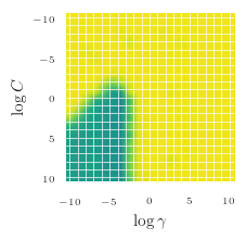
(a) $s=\nicefrac{{1}}{{128}}$

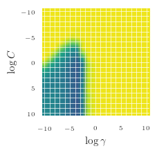
(b) $s=\nicefrac{{1}}{{16}}$

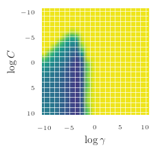
(c) $s=\nicefrac{{1}}{{4}}$

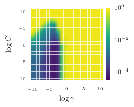
(d) $s=1$

Figure 1: Validation error of a grid of $400$ SVM configurations (20 settings of each of the regularization parameter $C$ and kernel parameter $\gamma$, both on a log-scale in $[-10,10]$) for subsets of the MNIST dataset (LeCun et al., 2001) of various sizes $N_{\text{sub}}$. Small subsets are quite representative: The validation error of bad configuration (yellow) remains constant at around $0.9$, whereas the region of good configurations (blue) does not change drastically with $s$.

For an initial intuition on how performance changes with dataset size, we evaluated a grid of $400$ configurations of a support vector machine (SVM) on subsets of the MNIST dataset (LeCun et al., 2001) ; MNIST has $N=50\,000$ data points and we evaluated relative subset sizes $s\in\{\nicefrac{{1}}{{512}},\nicefrac{{1}}{{256}},\nicefrac{{1}}{{128}},\ldots,\nicefrac{{1}}{{4}},\nicefrac{{1}}{{2}},1\}$. Figure 1 visualizes the validation error of these configurations on $s=\nicefrac{{1}}{{128}}$, $\nicefrac{{1}}{{16}}$, $\nicefrac{{1}}{{4}}$, and $1$. Evidently, just $\nicefrac{{1}}{{128}}$ of the dataset is quite representative and sufficient to locate a reasonable configuration. Additionally, there are no deceiving local optima on smaller subsets. Based on these observations, we expect that relatively small fractions of the dataset yield representative performances and therefore vary our relative size parameter $s$ on a logarithmic scale.

3.1 Kernels for loss and computational cost

To transfer the insights from this illustrative example into a formal model for the loss and cost across subset sizes, we extend the GP model by an additional input dimension, namely $s\in[0,1]$. This allows the surrogate to extrapolate to the full data set at $s=1$ without necessarily evaluating there. We chose a factorized kernel, consisting of the standard stationary kernel over hyperparameters, multiplied with a finite-rank (“degenerate”) covariance function in $s$:

$$k\left(({\bm{x}},s),({\bm{x}}^{\prime},s^{\prime})\right)=k_{\nicefrac{{5}}{{2}}}\left({\bm{x}},{\bm{x}}^{\prime}\right)\cdot\left(\phi^{T}(s)\cdot\Sigma_{\phi}\cdot\phi(s^{\prime})\right)\,.$$ (6)

Since any choice of the basis function $\phi$ yields a positive semi-definite covariance function, this provides a flexible language for prior knowledge relating to $s$. We use the same form of kernel to model the loss $f$ and cost $c$, respectively, but with different basis functions $\phi_{f}$ and $\phi_{c}$.

The loss of a machine learning algorithms usually decreases with more training data. We incorporate this behavior by choosing $\phi_{f}(s)=(1,(1-s)^{2})^{T}$ to enforce monotonic predictions with an extremum at $s=1$. This kernel choice is equivalent to Bayesian linear regression with these basis functions and Gaussian priors on the weights.

To model computational cost $c$, we note that the complexity usually grows with relative dataset size $s$. To fit polynomial complexity $\mathcal{O}(s^{\alpha})$ for arbitrary $\alpha$ and simultaneously enforce positive predictions, we model the log-cost and use $\phi_{c}(s)=(1,s)^{T}$. As above, this amounts to Bayesian linear regression with shown basis functions.

In the supplemental material (Section B), we visualize scaling of loss and cost with $s$ for the SVM example above and show that our kernels indeed fit them well. We also evaluate the possibility of modelling the heteroscedastic noise introduced by subsampling the data (supplementary material, Section C).

3.2 Formal algorithm description

Fabolas starts with an initial design, described in more detail in Section 3.3. Afterwards, at the beginning of each iteration it fits GPs for loss and computational cost across dataset sizes $s$ using the kernel from Eq. 6. Then, capturing the distribution of the optimum for $s=1$ using $p_{\min}^{s=1}({\bm{x}}\mid\mathcal{D}):=p({\bm{x}}\in\operatornamewithlimits{arg\,min}_{{\bm{x}}^{\prime}\in\mathbb{X}}f({\bm{x}}^{\prime},s=1)\mid\mathcal{D})$, it selects the maximizer of the following acquisition function to trade off information gain versus cost:

$$a_{\text{F}}({\bm{x}},s): =\frac{1}{c({\bm{x}},s)+c_{\text{overhead}}}$$

$$\mathbb{E}_{p(y\mid{\bm{x}},s,\mathcal{D})}\left[\int p_{\min}^{s=1}({\bm{x}}^{\prime}\mid\mathcal{D}\cup\{({\bm{x}},s,y)\})\cdot\right.$$ (7)

$$\left.\log\frac{p_{\min}^{s=1}({\bm{x}}^{\prime}\mid\mathcal{D}\cup\{({\bm{x}},s,y)\})}{u({\bm{x}}^{\prime})}\ \mathrm{d}{\bm{x}}^{\prime}\right].$$

Algorithm 1 shows pseudocode for Fabolas. We also provide an open-source implementation at https://github.com/automl/RoBO.

Algorithm 1 Fast BO for Large Datasets (Fabolas)

1:  Initialize data $\mathcal{D}_{0}$ using an initial design.

2:  for $t=1,2,\dots$ do

3:     Fit GP models for $f({\bm{x}},s)$ and $c({\bm{x}},s)$ on data $\mathcal{D}_{t-1}$

4:     Choose $({\bm{x}}_{t},s_{t})$ by maximizing the acquisition function in Equation 7.

5:     Evaluate $y_{t}\sim f({\bm{x}}_{t},s_{t})+\mathcal{N}(0,\sigma^{2})$, also measuring cost $z_{t}\sim c({\bm{x}}_{t},s_{t})+\mathcal{N}(0,\sigma^{2}_{c})$, and augment the data: $\mathcal{D}_{t}=\mathcal{D}_{t-1}\cup\{({\bm{x}}_{t},s_{t},y_{t},z_{t})\}$

6:     Choose incumbent $\hat{{\bm{x}}}_{t}$ based on the predicted loss at $s=1$ of all $\{{\bm{x}}_{1},{\bm{x}}_{2},\dots,{\bm{x}}_{t}\}$.

7:  end for

Our proposed acquisition function resembles the one used by MTBO (Eq. 2.3), with two differences: First, MTBO’s discrete tasks $t$ are replaced by a continuous dataset size $s$ (allowing to learn correlations without evaluations at $s=1$, and to choose the appropriate subset size automatically). Second, the prediction of computational cost is augmented by the overhead of the Bayesian optimization method. This inclusion of the reasoning overhead is important to appropriately reflect the information gain per unit time spent: it does not matter whether the time is spent with a function evaluation or with reasoning about which evaluation to perform. In practice, due to cubic scaling in the number of data points of GPs and the computational complexity of approximating $p_{\min}^{s=1}$, the additional overhead of Fabolas is within the order of minutes, such that differences in computational cost in the order of seconds become negligible in comparison.

Being an anytime algorithm, Fabolas keeps track of its incumbent at each time step. To select a configuration that performs well on the full dataset, it predicts the loss of all evaluated configurations at $s=1$ using the GP model and picks the minimizer. We found this to work more robustly than globally minimizing the posterior mean, or similar approaches.

3.3 Initial design

It is common in Bayesian optimization to start with an initial design of points chosen at random or from a Latin hypercube design to allow for reasonable GP models as starting points. To fully leverage the speedups we can obtain from evaluating small datasets, we bias this selection towards points with small (cheap) datasets in order to improve the prediction for dependencies on $s$: We draw $k$ random points in $\mathbb{X}$ ($k=10$ in our experiments) and evaluate them on different subsets of the data (for instance on the support vector machine experiments we used $s\in\{\nicefrac{{1}}{{64}},\nicefrac{{1}}{{32}},\nicefrac{{1}}{{16}},\nicefrac{{1}}{{8}}\}$). This provides information on scaling behavior, and, assuming that costs increase linearly or superlinearly with $s$, these $k$ function evaluations cost less than $\frac{k}{8}$ function evaluations on the full dataset. This is important as the cost of the initial design, of course, counts towards Fabolas’ runtime.

3.4 Implementation details

The presentation of Fabolas above omits some details that impact the performance of our method. As it has become standard in Bayesian optimization (Snoek et al., 2012), we use Markov-Chain Monte Carlo (MCMC) integration to marginalize over the GPs hyperparameters (we use the emcee package (Foreman-Mackey et al., 2013)). To accelerate the optimization, we use hyper-priors to emphasize meaningful values for the parameters, chiefly adopting the choices of the spearmint toolbox (Snoek et al., 2012): a uniform prior between $[-10,2]$ for all length scales ${\bm{\lambda}}$ in log space, a lognormal prior ($\mu_{a}=0$, $\sigma_{a}^{2}=1$) for the covariance amplitude $\theta$, and a horseshoe prior with length scale of $0.1$ for the noise variance $\sigma^{2}$.

We used the original formulation of ES by Hennig and Schuler (2012) rather than the recent reformulation of PES by Hernández-Lobato et al. (2014). The main reason for this is that the latter prohibits non-stationary kernels due to its use of Bochner’s theorem for a spectral approximation. PES could in principle be extended to work for our particular choice of kernels (using an Eigen-expansion, from which we could sample features); since this would complicate making modifications to our kernel, we leave it as an avenue for future work, but note that in any case it may only further improve our method. To maximize the acquisition function we used the blackbox optimizer DIRECT (Jones, 2001) and CMAES (Hansen, 2006).

4 Experiments

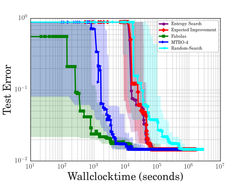
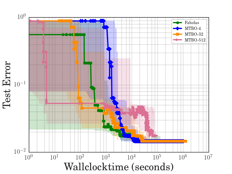
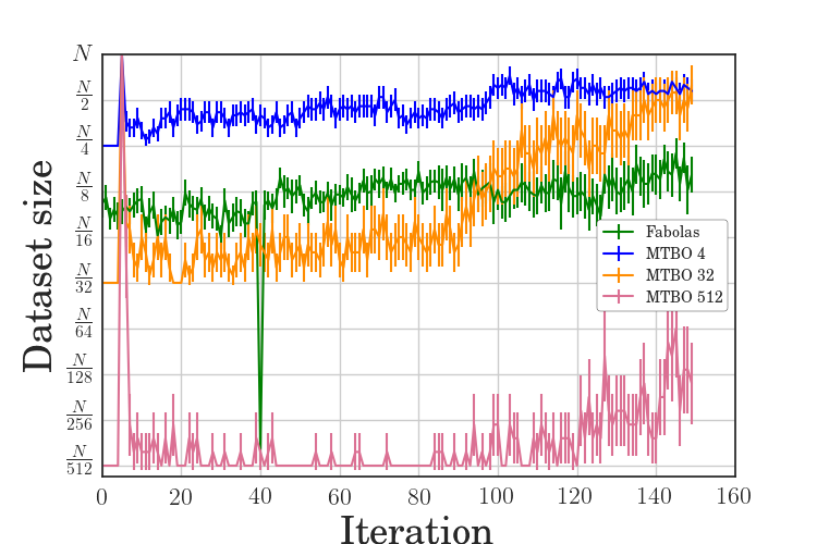
Figure 2: Evaluation on SVM grid on MNIST. (Left) Baseline comparison of test performance of the methods’ selected incumbents over time. (Middle) Test performance over time for variants of MTBO with different dataset sizes for the auxiliary task. (Right) Dataset size Fabolas and MTBO pick in each iteration to trade off small cost and high information gain; unlike elsewhere in the paper, this right plot shows mean $\pm\nicefrac{{1}}{{4}}$ stddev of $30$ runs (medians would only take two values for MTBO).

For our empirical evaluation of Fabolas, we compared it to standard Bayesian optimization (using EI and ES as acquisition functions), MTBO, and Hyperband. For each method, we tracked wall clock time (counting both optimization overhead and the cost of function evaluations, including the initial design), storing the incumbent returned after every iteration. In an offline validation step, we then trained models with all incumbents on the full dataset and measured their test error. We plot these test errors throughout. To obtain error bars, we performed 10 independent runs of each method with different seeds (except on the grid experiment, where we could afford 30 runs per method) and plot medians, along with ${25}^{\text{th}}$ and $75^{\text{th}}$ percentiles for all experiments. Details on the hyperparameter ranges used in every experiment are given in the supplemental material (Section D).

We implemented Hyperband following Li et al. (2017) using the recommended setting for the parameter $\eta=3$ that controls the intermediate subset sizes. For each experiment, we adjusted the budget allocated to each Hyperband iteration to allow the same minimum dataset size as for Fabolas: 10 times the number of classes for the support vector machine benchmarks and the maximum batch size for the neural network benchmarks. We also followed the prescribed incumbent estimation after each iteration as the configuration with the best performance on the full dataset size.

4.1 Support vector machine grid on MNIST

First, we considered a benchmark allowing the comparison of the various Bayesian optimization methods on ground truth: our SVM grid on MNIST (described in Section 3), for which we had performed all function evaluations beforehand, measuring loss and cost 10 times for each configuration ${\bm{x}}$ and subset size $s$ to account for performance variations. (In this case, we computed each method’s wall clock time in each iteration as its summed optimization overheads so far, plus the summed costs for the function values it queried so far.)

MTBO requires choosing the number of data points in its auxiliary task. Figure 2 (middle) evaluates MTBO variants with a single auxiliary task with a relative size of $\nicefrac{{1}}{{4}}$, $\nicefrac{{1}}{{32}}$, and $\nicefrac{{1}}{{512}}$, respectively. With auxiliary tasks at either $s=\nicefrac{{1}}{{512}}$ or $\nicefrac{{1}}{{32}}$, MTBO improved quickly, but converged more slowly to the optimum; we believe small correlations between the tasks cause this. Figure 2 (right) shows the dataset sizes chosen by the different algorithms during the optimization; all methods slowly increased the average subset size used over time. An auxiliary task with $s=\nicefrac{{1}}{{4}}$ worked best and we used this for MTBO in the remaining experiments.

At first glance, one might expect many tasks (e.g., with a task for each $s\in\{\nicefrac{{1}}{{512}},\nicefrac{{1}}{{256}},\dots,\nicefrac{{1}}{{2}},1\}$) to work best, but quite the opposite is true. In preliminary experiments, we evaluated MTBO with up to 3 auxiliary tasks ($s=\nicefrac{{1}}{{4}}$, $\nicefrac{{1}}{{32}}$, and $\nicefrac{{1}}{{512}}$), but found performance to strongly degrade with a growing number of tasks. We suspect that the ${|T|}\choose{2}$ kernel parameters that have to be learned for the discrete task kernel for $|T|$ tasks are the main reason. If the MCMC sampling is too short, the correlations are not appropriately reflected, especially in early iterations, and an adjusted sampling creates a large computational overhead that dominates wall-clock time. We therefore obtained best performance with only one auxiliary task.

Figure 2 (left) shows results using EI, ES, random search, MTBO and fabolas on this SVM benchmark. EI and ES perform equally well and find the best configuration (which yields an error of $0.014$, or $1.4\%$) after around $10^{5}$ seconds, roughly five times faster than random search. MTBO achieves good performance faster, requiring only around $2\times 10^{4}$ seconds to find the global optimum. Fabolas is roughly another order of magnitude faster than MTBO in finding good configurations, and finds the global optimum at the same time.

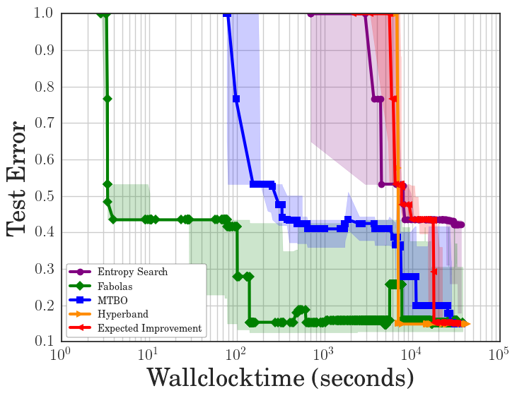
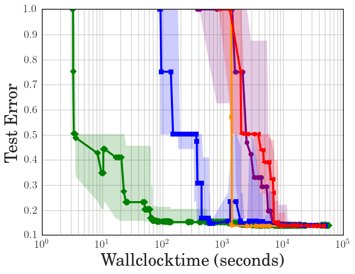
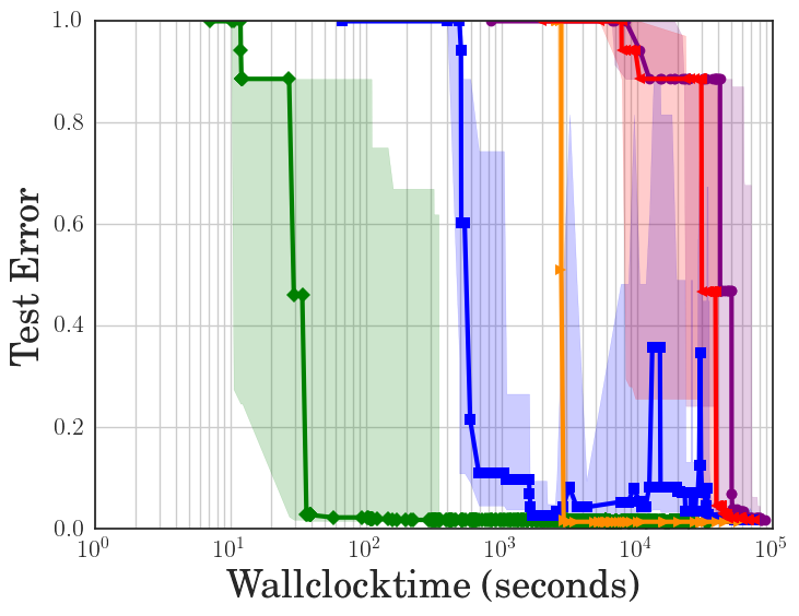
Figure 3: SVM hyperparameter optimization on the datasets covertype (left), vehicle (middle) and MNIST(right). At each time, the plots show test performance of the methods’ respective incumbents. Fabolas finds a good configuration between 10 and 1000 times faster than the other methods.

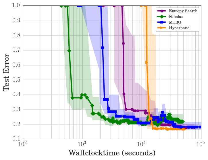
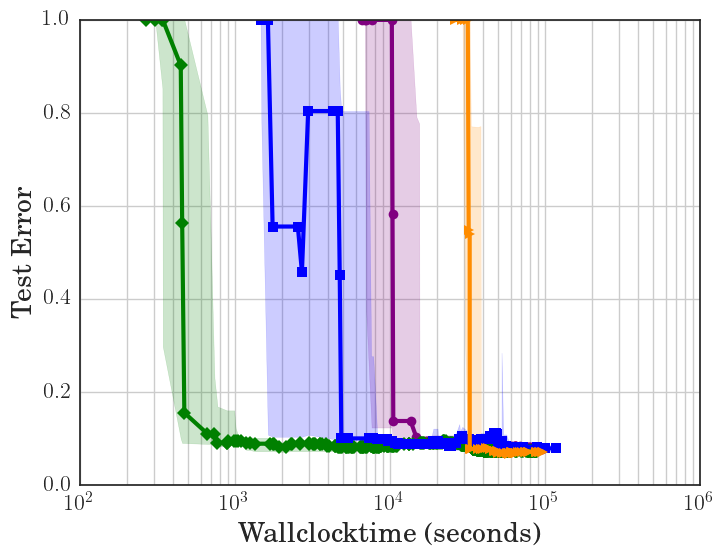
Figure 4: Test performance of a convolutional neural network on CIFAR10 (left) and SVHN (right).

4.2 Support vector machines on various datasets

For a more realistic scenario, we optimized the same SVM hyperparameters without a grid constraint on MNIST and two other prominent UCI datasets (gathered from OpenML (Vanschoren et al., 2014)), vehicle registration (Siebert, 1987) and forest cover types (Blackard and Dean, 1999) with more than 50000 data points, now also comparing to Hyperband. Training SVMs on these datasets can take several hours, and Figure 3 shows that Fabolas found good configurations for them between 10 and 1000 times faster than the other methods.

Hyperband required a relatively long time until it recommended its first hyperparameter setting, but this first recommendation was already very good, making Hyperband substantially faster to find good settings than standard Bayesian optimization running on the full dataset. However, Fabolas typically returned configurations with the same quality another order of magnitude faster.

4.3 Convolutional neural networks on CIFAR-10 and SVHN

Convolutional neural networks (CNNs) have shown superior performance on a variety of computer vision and speech recognition benchmarks, but finding good hyperparameter settings remains challenging, and almost no theoretical guarantees exist. Tuning CNNs for modern, large datasets is often infeasible via standard Bayesian optimization; in fact, this motivated the development of Fabolas.

We experimented with hyperparameter optimization for CNNs on two well-established object recognition datasets, namely CIFAR10 (Krizhevsky, 2009) and SVHN (Netzer et al., 2011). We used the same setup for both datasets (a CNN with three convolutional layers, with batch normalization (Ioffe and Szegedy, 2015) in each layer, optimized using Adam (Kingma and Ba, 2014)). We considered a total of five hyperparameters: the initial learning rate, the batch size and the number of units in each layer. For CIFAR10, we used 40000 images for training, 10000 to estimate validation error, and the standard 10000 hold-out images to estimate the final test performance of incumbents. For SVHN, we used 6000 of the 73257 training images to estimate validation error, the rest for training, and the standard 26032 images for testing.

The results in Figure 4 show that—compared to the SVM tasks—Fabolas’ speedup was smaller because CNNs scale linearly in the number of datapoints. Nevertheless, it found good configurations about 10 times faster than vanilla Bayesian optimization. For the same reason of linear scaling, Hyperband was substantially slower than vanilla Bayesian optimization to make a recommendation, but it did find good hyperparameter settings when given enough time.

4.4 Residual neural network on CIFAR-10

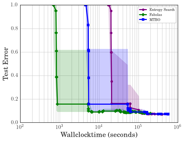
Figure 5: Validation performance of a residual network on CIFAR10.

In the final experiment, we evaluated the performance of our method further on a more expensive benchmark, optimizing the validation performance of a deep residual network on the CIFAR10 dataset, using the original architecture from He et al. (2015). As hyperparameters we exposed the learning rate, $L_{2}$ regularization, momentum and the factor by which the learning rate is multiplied after $41$ and $61$ epochs.

Figure 5 shows that Fabolas found configurations with reasonable performance roughly 10 times faster than ES and MTBO. Note that due to limited computational capacities, we were unable to run Hyperband on this benchmark: a single iteration took longer than a day, making it prohibitively expensive. (Also note that by that time all other methods had already found good hyperparameter settings.) We want to emphasize that the runtime could be improved by adapting Hyperband’s parameters to the benchmark, but we decided to keep all methods’ parameters fixed throughout the experiments to also show their robustness.

5 Conclusion

We presented Fabolas, a new Bayesian optimization method based on entropy search that mimics human experts in evaluating algorithms on subsets of the data to quickly gather information about good hyperparameter settings. Fabolas extends the standard way of modelling the objective function by treating the dataset size as an additional continuous input variable. This allows the incorporation of strong prior information. It models the time it takes to evaluate a configuration and aims to evaluate points that yield—per time spent—the most information about the globally best hyperparameters for the full dataset. In various hyperparameter optimization experiments using support vector machines and deep neural networks, Fabolas often found good configurations 10 to 100 times faster than the related approach of Multi-Task Bayesian optimization, Hyperband and standard Bayesian optimization. Our open-source code is available at https://github.com/automl/RoBO, along with scripts for reproducing our experiments.

In future work, we plan to expand our algorithm to model other environmental variables, such as the resolution size of images, the number of classes, and the number of epochs, and we expect this to yield additional speedups. Since our method reduces the cost of individual function evaluations but requires more of these cheaper evaluations, we expect the cubic complexity of Gaussian processes to become the limiting factor in many practical applications. We therefore plan to extend this work to other model classes, such as Bayesian neural networks (Neal, 1996; Hernández-Lobato and Adams, 2015; Blundell et al., 2015; Springenberg et al., 2016; Klein et al., 2017), which may lower the computational overhead while having similar predictive quality.

References

- Montavon et al. (2012) G. Montavon, G. Orr, and K.-R. Müller, editors. Neural Networks: Tricks of the Trade - Second Edition. LNCS. Springer, 2012.
- Bergstra et al. (2011) J. Bergstra, R. Bardenet, Y. Bengio, and B. Kégl. Algorithms for hyper-parameter optimization. In Proc. of NIPS’11, 2011.
- Hutter et al. (2011) F. Hutter, H. Hoos, and K. Leyton-Brown. Sequential model-based optimization for general algorithm configuration. In Proc. of LION’11, 2011.
- Bergstra and Bengio (2012) J. Bergstra and Y. Bengio. Random search for hyper-parameter optimization. JMLR, 2012.
- Snoek et al. (2012) J. Snoek, H. Larochelle, and R. P. Adams. Practical Bayesian optimization of machine learning algorithms. In Proc. of NIPS’12, 2012.
- Bardenet et al. (2013) R. Bardenet, M. Brendel, B. Kégl, and M. Sebag. Collaborative hyperparameter tuning. In Proc. of ICML’13, 2013.
- Bergstra et al. (2013) J. Bergstra, D. Yamins, and D. Cox. Making a science of model search: Hyperparameter optimization in hundreds of dimensions for vision architectures. In Proc. of ICML’13, 2013.
- Swersky et al. (2013) K. Swersky, J. Snoek, and R. Adams. Multi-task Bayesian optimization. In Proc. of NIPS’13, 2013.
- Swersky et al. (2014) K. Swersky, J. Snoek, and R. Adams. Freeze-thaw Bayesian optimization. CoRR, 2014.
- (10) J. Snoek, K. Swersky, R. Zemel, and R. Adams. Input warping for Bayesian optimization of non-stationary functions. In Proc. of ICML’14.
- Snoek et al. (2015) J. Snoek, O. Rippel, K. Swersky, R. Kiros, N. Satish, N. Sundaram, M. M. A. Patwary, Prabhat, and R. P. Adams. Scalable Bayesian optimization using Deep Neural Networks. In Proc. of ICML’15, 2015.
- Krizhevsky (2009) A. Krizhevsky. Learning multiple layers of features from tiny images. Technical report, University of Toronto, 2009.
- Domhan et al. (2015) T. Domhan, J. T. Springenberg, and F. Hutter. Speeding up automatic hyperparameter optimization of deep neural networks by extrapolation of learning curves. In Proc. of IJCAI’15, 2015.
- Bottou (2012) L. Bottou. Stochastic gradient tricks. In Grégoire Montavon, Genevieve B. Orr, and Klaus-Robert Müller, editors, Neural Networks, Tricks of the Trade, Reloaded. Springer, 2012.
- Nickson et al. (2014) T. Nickson, M. A Osborne, S. Reece, and S. Roberts. Automated machine learning on big data using stochastic algorithm tuning. CoRR, 2014.
- Krueger et al. (2015) T. Krueger, D. Panknin, and M. Braun. Fast cross-validation via sequential testing. JMLR, 2015.
- Li et al. (2016) L. Li, K. Jamieson, G. DeSalvo, A. Rostamizadeh, and A. Talwalkar. Efficient hyperparameter optimization and infinitely many armed bandits. 2016.
- (18) A. Klein, S. Bartels, S. Falkner, P. Hennig, and F. Hutter. Towards efficient Bayesian optimization for big data. In Proc. of BayesOpt’15.
- Li et al. (2017) L. Li, K. Jamieson, G. DeSalvo, A. Rostamizadeh, and A. Talwalkar. Hyperband: Bandit-based configuration evaluation for hyperparameter optimization. In Proc. of ICLR’17, 2017.
- Brochu et al. (2010) E. Brochu, V. Cora, and N. de Freitas. A tutorial on Bayesian optimization of expensive cost functions, with application to active user modeling and hierarchical reinforcement learning. CoRR, 2010.
- Shahriari et al. (2016) B. Shahriari, K. Swersky, Z. Wang, R. Adams, and N. de Freitas. Taking the human out of the loop: A Review of Bayesian Optimization. Proc. of the IEEE, (1), 12/2015 2016.
- Rasmussen and Williams (2006) C. Rasmussen and C. Williams. Gaussian Processes for Machine Learning. The MIT Press, 2006.
- Matérn (1960) B. Matérn. Spatial variation. Meddelanden fran Statens Skogsforskningsinstitut, 1960.
- MacKay and Neal (1994) D.J.C. MacKay and R.M. Neal. Automatic relevance detection for neural networks. Technical report, University of Cambridge, 1994.
- Mockus et al. (1978) J. Mockus, V. Tiesis, and A. Zilinskas. The application of Bayesian methods for seeking the extremum. Towards Global Optimization, (117-129), 1978.
- Srinivas et al. (2010) N. Srinivas, A. Krause, S. Kakade, and M. Seeger. Gaussian process optimization in the bandit setting: No regret and experimental design. In Proc. of ICML’10, 2010.
- Hennig and Schuler (2012) P. Hennig and C. Schuler. Entropy search for information-efficient global optimization. JMLR, (1), 2012.
- Hernández-Lobato et al. (2014) J. Hernández-Lobato, M. Hoffman, and Z. Ghahramani. Predictive entropy search for efficient global optimization of black-box functions. In Proc. of NIPS’14, 2014.
- Williams et al. (2000) B. Williams, T. Santner, and W. Notz. Sequential design of computer experiments to minimize integrated response functions. Statistica Sinica, 2000.
- LeCun et al. (2001) Y. LeCun, L. Bottou, Y. Bengio, and P. Haffner. Gradient-based learning applied to document recognition. In S. Haykin and B. Kosko, editors, Intelligent Signal Processing. IEEE Press, 2001.
- Foreman-Mackey et al. (2013) D. Foreman-Mackey, D. W. Hogg, D. Lang, and J. Goodman. emcee : The MCMC Hammer. PASP, 2013.
- Jones (2001) D. R. Jones. A taxonomy of global optimization methods based on response surfaces. JGO, 2001.
- Hansen (2006) N. Hansen. The CMA evolution strategy: a comparing review. In J.A. Lozano, P. Larranaga, I. Inza, and E. Bengoetxea, editors, Towards a new evolutionary computation. Advances on estimation of distribution algorithms. Springer, 2006.
- Vanschoren et al. (2014) J. Vanschoren, J. van Rijn, B. Bischl, and L. Torgo. OpenML: Networked science in machine learning. SIGKDD Explor. Newsl., (2), June 2014.
- Siebert (1987) J.P. Siebert. Vehicle Recognition Using Rule Based Methods. Turing Institute, 1987.
- Blackard and Dean (1999) J A Blackard and D J Dean. Comparative accuracies of artificial neural networks and discriminant analysis in predicting forest cover types from cartographic variables. Comput. Electron. Agric., 1999.
- Netzer et al. (2011) Y. Netzer, T. Wang, A. Coates, A. Bissacco, B. Wu, and A. Y. Ng. Reading digits in natural images with unsupervised feature learning. In NIPS Workshop on Deep Learning and Unsupervised Feature Learning 2011, 2011.
- Ioffe and Szegedy (2015) S. Ioffe and C. Szegedy. Batch normalization: Accelerating deep network training by reducing internal covariate shift. In Proceedings of the 32nd International Conference on Machine Learning,ICML 2015, Lille, France, 6-11 July 2015, 2015.
- Kingma and Ba (2014) D. P. Kingma and J. Ba. Adam: A method for stochastic optimization. CoRR, 2014.
- He et al. (2015) K. He, X. Zhang, S. Ren, and J. Sun. Deep residual learning for image recognition. CoRR, 2015.
- Neal (1996) R. Neal. Bayesian learning for neural networks. PhD thesis, University of Toronto, 1996.
- Hernández-Lobato and Adams (2015) J. Hernández-Lobato and R. Adams. Probabilistic backpropagation for scalable learning of Bayesian neural networks. In Proc. of ICML’15, 2015.
- Blundell et al. (2015) C. Blundell, J. Cornebise, K. Kavukcuoglu, and D. Wierstra. Weight uncertainty in neural networks. In Proc. of ICML’15, 2015.
- Springenberg et al. (2016) J. T. Springenberg, A. Klein, S. Falkner, and F. Hutter. Bayesian optimization with robust Bayesian neural networks. In Proc. of NIPS’16, 2016.
- Klein et al. (2017) A. Klein, S. Falkner, J. T. Springenberg, and F. Hutter. Learning curve prediction with Bayesian neural networks. In Proc. of ICLR’17, 2017.