Poynting-Robertson drag and solar wind in the space debris problem

Abstract

We analyze the combined effect of Poynting-Robertson and solar wind drag on space debris. We derive a model within Cartesian, Gaussian and Hamiltonian frameworks. We focus on the geosynchronous resonance, although the results can be easily generalized to any resonance. By numerical and analytical techniques, we compute the drift in semi-major axis due to Poynting-Robertson and solar wind drag. After a linear stability analysis of the equilibria, we combine a careful investigation of the regular, resonant, chaotic behavior of the phase space with a long-term propagation of a sample of initial conditions. The results strongly depend on the value of the area-to-mass ratio of the debris, which might show different dynamical behaviors: temporary capture or escape from the geosynchronous resonance, as well as temporary capture or escape from secondary resonances involving the rate of variation of the longitude of the Sun. Such analysis shows that Poynting-Robertson and solar wind drag must be taken into account, when looking at the long-term behavior of space debris. Trapping or escape from the resonance can be used to place the debris in convenient regions of the phase space.

keywords Poynting-Robertson effect, Solar wind, Geostationary orbit, Space debris

1 Introduction

The population of space debris shows a wide variety of different case studies: micro-metric particles to meter-size debris, small to large area-to-mass ratios, circular to highly inclined orbits, etc. These characteristics of the space debris, together with their actual location in LEO, MEO, GEO, lead to consider several models as well as a different hierarchy of the forces which contribute to shape the dynamics. For example, it was widely shown (see, e.g., Celletti & Galeş (2015), Kuznetsov (2011), Valk et al. (2009) and references therein) that the effect of solar radiation pressure on GEO and MEO objects is more relevant for larger area-to-mass ratios. The dissipative contribution due to Poynting-Robertson and solar wind is definitely considered much less important. However, such dissipative effects might become relevant on micro-meter size particles as well on large area-to-mass ratio space debris (various objects with high area-to-mass ratios are described, e.g., in Früh & Schildknecht (2012)).

The aim of the current study is to settle the question of the role of Poynting-Robertson and solar wind (hereafter PR/SW) drag on space debris dynamics. The relevance of this question stems from the consideration that the drag might provoke a drift of the debris towards space regions where operating satellites are placed. To avoid collisions with functional satellites and a consequent possible generation of further debris, it is crucial to have a full control of the dynamics of space debris, including the prediction over long time scales of minor, but still relevant, effects like PR/SW. Our study shows that not only Poynting-Robertson drag, but also solar wind drag, are prominent forces that need to be included in the model to get an accurate estimate of the drift of space debris in the near-Earth environment.

The first studies on the Poynting-Robertson effect in the artificial satellite problem date back to Slabinski (1980, 1983), where the author states that the semi-major axis of a near synchronous satellite with small area-to-mass ratio can decrease at a rate of about 1 $mt/yr$. The secular evolution of geostationary objects caused by light pressure alone has been treated in Smirnov & Mikisha (1993, 1995). Numerical simulations in the neighborhood of the 1:1, 1:2, and 1:3 resonances can be found in Kuznetsov et al. (2012, 2013). The authors estimate the secular effect caused by the Poynting-Robertson drag for various area-to-mass ratios being of the order of hundreds of meters per year, approximately. In Kuznetsov et al. (2014) the authors provide a series of numerically obtained estimates of drift rates for various high order resonances close to the geosynchronous orbit. They find drift rates (in absolute magnitudes) ranging from about 29 $mt/yr$ (9:11 resonance) to about 142 $mt/yr$ (5:4 resonance) with a variation of 33 $mt/yr$ to 75 $mt/yr$ close to the geosynchronous orbit (see Table 2 in Kuznetsov et al. (2014)). Secular rates of drift in semi-major axis of about 500 $mt/yr$ have also numerically been estimated in Kuznetsov & Zakharova (2015) for high area-to-mass ratio objects in highly elliptical orbits, the so-called Molniya orbits, close to the 22:45 resonance.

As it has been recognized in Kuznetsov (2011), drift rates in the vicinity of the geosynchronous orbit may differ by orders of magnitude. Typical estimates for standard area-to-mass ratios range from -23 $km/yr$ (Smirnov & Mikisha, 1993), -59 $mt/yr$ (Slabinski, 1980), -51 $mt/yr$ (Tueva & Avdyushev, 2006), and -80 $mt/yr$ (all values taken from Kuznetsov, 2011). The divergence is clearly due to resonance effects, so that the drift in semi-major axis strongly depends on the initial condition, i.e. the distance from the exact resonance, that itself becomes shifted for large area-to-mass ratios.

The aim of our study is to provide a detailed investigation of the drift in semi-major axis of space debris of high area-to-mass ratios, subject to the lower degree gravitational field of the Earth, the gravitational attraction due to the Moon and the Sun, direct solar radiation pressure, the Poynting-Robertson drag and the solar wind drag forces. First, we provide the model in different frameworks: Cartesian coordinates, Gaussian equations of motion and using a Hamiltonian approach. We investigate the dynamics by means of secular perturbation theory, and isolate the effects due to PR/SW-drag from additional perturbations of Kepler’s orbit. We provide realistic estimates of the drift by means of simple formulae and check our results by means of a numerical integration of the full problem.

On the basis of a newly developed, fully non-resonant secular theory, our estimate of the drift rate outside the geosynchronous resonant regime of motion turns out to be of the order of 40 $mt/yr$, a value which is confirmed by numerical experiments. Averaging over the fast variables, one obtains a simple system of equations which allows us to compute the location of the equilibria for the geostationary orbit, within different models, possibly including Poynting-Robertson effect and solar wind. Under the influence of dissipative forces, we find different behaviors in the neighborhood of the geosynchronous resonance: we find temporary capture, with a transient time varying according to the orbital properties and to the value of the area-to-mass ratio; we observe escape orbits or rather transitions between the main resonance and other resonances involving the rate of variation of the longitude of the Sun. Our investigation includes a detailed study of possible chaotic motions at the border of the resonance; such regions might be used to transfer the debris without much effort, but rather relying on the dynamical properties of the chaotic regions.

We mention that to get a comprehensive description of the dynamics, other effects should have been considered. Among the others, we mention the long-term periodic evolution of space debris trajectories caused by successive Earth’s shadow crossings, which has been investigated, e.g., in Hubaux & Lemaître (2013); a detailed model of the so-called BYORP effect, which has been derived in McMahon & Scheeres (2010).

This paper is organized as follows. In Section 2 we present the dynamical model we are going to use, and derive the geocentric formulation of PR/SW-drag. A qualitative discussion of the PR/SW-drag on artificial satellite motion can be found in Section 3. The detailed investigation of the dynamics close to the resonant regimes of motion is provided in Section 4. A discussion of the results can be found in Section 5.

2 The dynamical model

In this Section we present a model describing the motion of a spherical space debris object (hereafter SDO) subject to the gravitational influence of the Earth, the gravitational attraction of the Moon, and the Sun, solar radiation pressure, solar wind, and Poynting-Robertson drag force. The Cartesian formulation is given in Section 2.1, the Gaussian equations of motion are presented in Section 2.2, while a Hamiltonian description is given in Section 2.3.

2.1 Cartesian framework

Let $\vec{r}$ be the position of the SDO of mass $m$ in a quasi-inertial, geocentric reference frame, $\mathbf{e}=(\vec{e}_{1},\vec{e}_{2},\vec{e}_{3})$, and denote by $\vec{r}_{M}$, $\vec{r}_{S}$ the position vectors of the Moon, and the Sun, respectively. Then, the equation of motion of the SDO is given by:

$$\frac{d^{2}\vec{r}}{dt^{2}}=-\frac{d}{d\vec{r}}\bigg{[}V_{E}\left(\vec{r}\right)+V_{M}\left(\vec{r},\vec{r}_{M}\right)+V_{S}\left(\vec{r},\vec{r}_{S}\right)+V_{SRP}\left(\vec{r},\vec{r}_{S}\right)\bigg{]}+\vec{F}_{PR/SW}\left(\vec{r},\vec{r}_{S}\right)\ ,$$ (1)

where $V_{E}$, $V_{M}$, $V_{S}$ are the gravitational potentials of the Earth, the Moon, and the Sun, $V_{SRP}$ is the potential of solar radiation pressure, and $\vec{F}_{PR/SW}$ labels the combined Poynting-Robertson and solar wind drag terms, respectively. Let $\mu={\mathcal{G}}m_{E}$ be the geocentric gravitational constant with constant of gravity ${\mathcal{G}}$, and mass of the Earth $m_{E}$. The geopotential $V_{E}$ is given in a synodic reference frame, with unit vectors $\mathbf{f}=(\vec{f}_{1},\vec{f}_{2},\vec{f}_{3})$, and rotating with the same angular velocity of the Earth, as (Montenbruck & Gill (2000)):

$$V_{E}(r,\phi,\lambda)={{{\mathcal{G}}m_{E}}\over r}\ \sum_{n=0}^{\infty}\Big{(}{R_{E}\over r}\Big{)}^{n}\ \sum_{m=0}^{n}P_{nm}(\sin\phi)\ (C_{nm}\cos m\lambda+S_{nm}\sin m\lambda)\ .$$

Here $r$, $\phi,\lambda$ are Earth-fixed spherical coordinates (radius, co-latitude, and longitude with $\lambda=0$ corresponding to the Greenwich mean meridian), and $R_{E}$, $C_{nm}$, $S_{nm}$ are the mean equatorial radius of the Earth and the (not normalized) Stokes coefficients that enter the spherical expansion of the Earth’s gravitational field up to degree $n$ and order $m$. The quantities $P_{nm}$ are the associated Legendre polynomials (in the geophysical sense, see Appendix A). We denote by $m_{M}$, $m_{S}$ the masses of the Moon and the Sun, respectively. The gravitational potentials due to the third-body, point-mass like interactions take the functional form (Murray & Dermott (1999)):

$$V_{k}\left(\vec{r},\vec{r}_{k}\right)={\mathcal{G}}m_{k}\left(\frac{1}{\|\vec{r}-\vec{r}_{k}\|}-\frac{\vec{r}\cdot\vec{r}_{k}}{r_{k}^{3}}\right)\ ,$$

with index $k=M$ for the Moon and $k=S$ for the Sun. We are left to provide $V_{SRP}$ and $F_{PR/SW}$. Let $\vec{X}$, $\vec{V}$, $R$ denote the position, velocity, and heliocentric distance of the SDO in the heliocentric frame of reference $\mathbf{g}=({\vec{g}}_{1},{\vec{g}}_{2},{\vec{g}}_{3})$, respectively. Furthermore, we denote by ${\hat{g}}_{R}=\vec{X}/{R}$ the radial unit vector along the line connecting Sun - SDO. The standard definition of the combined acceleration due to solar radiation pressure, Poynting-Robertson, and solar wind drag force, say ${\vec{F}^{\prime}}$, is given by (Burns et al. (1979); Klačka (2014); Lhotka & Celletti (2015)):

$$\vec{F^{\prime}}=\frac{\beta{\mathcal{G}}m_{S}}{{R}^{2}}\left[{\hat{g}}_{R}-\left(1+\frac{\eta}{Q}\right)\left(\frac{\vec{V}\cdot\hat{g}_{R}}{c}\ \hat{g}_{R}+\frac{\vec{V}}{c}\right)\right]\ .$$ (2)

Here, $\beta$ is the ratio of the magnitude of radiation force over solar gravitational attraction (Kocifaj et al. (2006)):

$$\beta=\frac{SQA}{c}/\frac{{\mathcal{G}}mm_{S}}{{R}^{2}}\simeq 7.6\times 10^{-4}\ Q\ \frac{A\ [mt^{2}]}{m\ [kg]}\ ,$$

with energy flux constant $S$, spectrally averaged dimensionless efficiency factor for radiation pressure $Q$, speed of light $c$, and the area cross section $A$ and mass $m$ of the SDO, respectively. In addition, $\eta$ in (2) is the dimensionless solar wind drag efficiency factor, i.e. the ratio of solar wind over Poynting-Robertson drag force (approximately about equal to $1/3$).

As a first step, we express (2) in the geocentric frame $\mathbf{e}$ by making use of the relation $\vec{X}=\vec{r}-\vec{r}_{S}$:

$$\vec{F^{\prime}}=\beta{\mathcal{G}}m_{S}\ {{\vec{r}-\vec{r}_{S}}\over{|\vec{r}-\vec{r}_{S}|^{3}}}-\frac{\beta{\mathcal{G}}m_{S}}{c}\left(1+\frac{\eta}{Q}\right)\left\{{{\vec{r}-\vec{r}_{S}}\over{|\vec{r}-\vec{r}_{S}|^{3}}}(\vec{\dot{r}}-\vec{\dot{r}}_{S})+{{\vec{\dot{r}}-\vec{\dot{r}}_{S}}\over{|\vec{r}-\vec{r}_{S}|^{2}}}\right\}\ .$$ (3)

We notice that the first term of (3) can be derived from the potential

$$V_{SRP}\left(\vec{r},\vec{r}_{S}\right)=\beta{\mathcal{G}}m_{S}\left(\frac{1}{|\vec{r}-\vec{r}_{S}|}\right)\ .$$

For clarity of exposition we split the conservative contribution from (3), and define the remaining force component ${\vec{F}}_{PR/SW}$ in (1) as:

$${\vec{F}}_{PR/SW}={\vec{F}^{\prime}}-\frac{dV_{SRP}\left(\vec{r},\vec{r}_{S}\right)}{d\vec{r}}\ .$$ (4)

Denoting by $(x,y,z)$, $(x_{M},y_{M},z_{M})$, $(x_{S},y_{S},z_{S})$ the coordinates in the quasi–inertial frame $\mathbf{e}$ of the SDO, Moon and Sun, respectively, the components of the equations of motion are then simply given by:

$$\ddot{x} = V_{x}(x,y,z,\theta)-{\mathcal{G}}m_{S}\Bigl{(}{{x-x_{S}}\over{|\vec{r}-\vec{r}_{S}|^{3}}}+{x_{S}\over r_{S}^{3}}\Bigr{)}-{\mathcal{G}}m_{M}\Bigl{(}{{x-x_{M}}\over{|\vec{r}-\vec{r}_{M}|^{3}}}+{x_{M}\over r_{M}^{3}}\Bigr{)}+\beta{\mathcal{G}}m_{S}\ {{x-x_{S}}\over{|\vec{r}-\vec{r}_{S}|^{3}}}\ -$$

$$\frac{\beta{\mathcal{G}}m_{S}}{c}\left(1+\frac{\eta}{Q}\right)\left\{{{x-x_{S}}\over{|\vec{r}-\vec{r}_{S}|^{3}}}(\dot{x}-\dot{x}_{S})+{{\dot{x}-\dot{x}_{S}}\over{|\vec{r}-\vec{r}_{S}|^{2}}}\right\}$$

$$\ddot{y} = V_{y}(x,y,z,\theta)-{\mathcal{G}}m_{S}\Bigl{(}{{y-y_{S}}\over{|\vec{r}-\vec{r}_{S}|^{3}}}+{y_{S}\over r_{S}^{3}}\Bigr{)}-{\mathcal{G}}m_{M}\Bigl{(}{{y-y_{M}}\over{|\vec{r}-\vec{r}_{M}|^{3}}}+{y_{M}\over r_{M}^{3}}\Bigr{)}+\beta{\mathcal{G}}m_{S}\ {{y-y_{S}}\over{|\vec{r}-\vec{r}_{S}|^{3}}}\ -$$

$$\frac{\beta{\mathcal{G}}m_{S}}{c}\left(1+\frac{\eta}{Q}\right)\left\{{{y-y_{S}}\over{|\vec{r}-\vec{r}_{S}|^{3}}}(\dot{y}-\dot{y}_{S})+{{\dot{y}-\dot{y}_{S}}\over{|\vec{r}-\vec{r}_{S}|^{2}}}\right\}$$

$$\ddot{z} = V_{z}(x,y,z,\theta)-{\mathcal{G}}m_{S}\Bigl{(}{{z-z_{S}}\over{|\vec{r}-\vec{r}_{S}|^{3}}}+{z_{S}\over r_{S}^{3}}\Bigr{)}-{\mathcal{G}}m_{M}\Bigl{(}{{z-z_{M}}\over{|\vec{r}-\vec{r}_{M}|^{3}}}+{z_{M}\over r_{M}^{3}}\Bigr{)}+\beta{\mathcal{G}}m_{S}\ {{z-z_{S}}\over{|\vec{r}-\vec{r}_{S}|^{3}}}\ -$$ (5)

$$\frac{\beta{\mathcal{G}}m_{S}}{c}\left(1+\frac{\eta}{Q}\right)\left\{{{z-z_{S}}\over{|\vec{r}-\vec{r}_{S}|^{3}}}(\dot{z}-\dot{z}_{S})+{{\dot{z}-\dot{z}_{S}}\over{|\vec{r}-\vec{r}_{S}|^{2}}}\right\}\ ,$$

where $(V_{x},V_{y},V_{z})$ represent the three components of the derivatives of the geopotential in the sidereal reference frame $\mathbf{e}$ that depend, additionally, on the sidereal time $t$ through the Greenwich Meridian angle $\theta$. The system of equations (2.1) serves as the basis for our numerical study.

2.2 Gauss’ form of the equations of motions

For the qualitative description of the secular dynamics of the SDO we will also work in Kepler elements and Delaunay variables. Let $a$ be the semi-major axis, $e$ the eccentricity, $i$ the inclination, $\omega$ be the argument of perihelion, $\Omega$ the longitude of the ascending node, and $M$ the mean anomaly defined in the quasi-inertial reference frame $\mathbf{e}$. In this setting, the norm of the orbital angular momentum is given by $h=\sqrt{1-e^{2}}\sqrt{\mu a}$, Kepler’s 3rd law is $\mu=n^{2}a^{3}$, and $n$ is the mean motion of the SDO. We start with Gauss’ form of the perturbed Kepler equations of motion (Fitzpatrick (1970)):

$$\frac{da}{dt} = \frac{2ah}{\mu\left(1-e^{2}\right)}\left[e\sin f{\mathfrak{F}}_{R}+\left(1+e\cos f\right){\mathfrak{F}}_{T}\right]\ ,$$ (6)

$$\frac{de}{dt} = \frac{h}{\mu}\left[\sin f{\mathfrak{F}}_{R}+\left(\cos f+\cos E\right){\mathfrak{F}}_{T}\right]\ ,$$

$$\frac{di}{dt} = \frac{\cos\left(\omega+f\right)r}{h}{\mathfrak{F}}_{N},\$$

$$\frac{d\omega}{dt} = -\frac{h}{\mu}\frac{1}{e}\left[\cos f{\mathfrak{F}}_{R}-\left(\frac{2+e\cos f}{1+ecosf}\right)\sin f{\mathfrak{F}}_{T}\right]-\frac{\cos i\sin\left(\omega+f\right)r{\mathfrak{F}}_{N}}{h\sin i}\ ,$$

$$\frac{d\Omega}{dt} = \frac{\sin\left(\omega+f\right)r}{h\sin i}{\mathfrak{F}}_{N}\ ,$$

$$\frac{dM}{dt} = n+\frac{h}{\mu}\frac{\sqrt{1-e^{2}}}{e}\left[\left(\cos f-\frac{2e}{1-e^{2}}\frac{r}{a}\right){\mathfrak{F}}_{R}-\left(1+\frac{1}{1-e^{2}}\frac{r}{a}\right)\sin f{\mathfrak{F}}_{T}\right]\ .$$

Here, $\mathfrak{F}_{R}$, $\mathfrak{F}_{T}$, $\mathfrak{F}_{N}$ are the radial, tangential, and normal components of a generic perturbing force, decomposed in the form:

$${\mathfrak{F}}=\mathfrak{F}_{R}{\mathbf{o}}_{R}+\mathfrak{F}_{T}{\mathbf{o}}_{T}+\mathfrak{F}_{N}{\mathbf{o}}_{N}\ ,$$ (7)

where ${\mathbf{o}}_{R}=(\cos f,\sin f,0)$, ${\mathbf{o}}_{T}=(-\sin f,\cos f,0)$, and ${\mathbf{e}}_{N}={\mathbf{o}}_{R}\times{\mathbf{o}}_{T}$ are the radial, tangential, and normal unit vectors defined in the orbital reference frame $\mathbf{o}$ centered at $\vec{r}$ with true anomaly $f$. The transformation between $\mathbf{o}$ and $\mathbf{e}$ is given in terms of the rotation matrix

$${\mathfrak{R}}={\mathfrak{R}}_{3}(\Omega)\cdot{\mathfrak{R}}_{1}(i)\cdot{\mathfrak{R}}_{3}(\omega)\ .$$

In this setting, the force function $\mathfrak{F}$ in (7) is related to ${\vec{F}}_{PR/SW}=F_{x}{\vec{e}}_{1}+F_{y}{\vec{e}}_{2}+F_{z}{\vec{e}}_{3}$ in (4), by the expressions (Moulton (1914)):

$$\mathfrak{F}_{R}=\left(F_{x},F_{y},F_{z}\right)\cdot{\mathfrak{R}}\cdot{\mathbf{o}}_{R}\ ,\ \mathfrak{F}_{T}=\left(F_{x},F_{y},F_{z}\right)\cdot{\mathfrak{R}}\cdot{\mathbf{o}}_{T}\ ,\ \mathfrak{F}_{N}=\left(F_{x},F_{y},F_{z}\right)\cdot{\mathfrak{R}}\cdot{\mathbf{o}}_{N}\ .$$

We remark, that using well known formulae for Taylor series expansions in the two-body problem (see, e.g., Dvorak & Lhotka (2013)), the right hand sides of (6) can be written in terms of the orbital elements of the SDO and the Sun, only.

2.3 Near Hamiltonian form

Let $L=\sqrt{\mu a}$, $G=L\sqrt{1-e^{2}}$, $H=G\cos i$, $l=M$, $g=\omega$, $h=\Omega$ denote the Delaunay variables of the SDO. The evolution in time of these action-angle like variables can be computed from (6) and take the following expression:

$$\frac{dL}{dt} = \frac{\mu}{2L}\frac{da}{dt}=-\frac{d\mathfrak{H}}{dl}+{\mathfrak{f}}_{L}\ ,$$

$$\frac{dG}{dt} = \frac{\mu G}{2L^{2}}\frac{da}{dt}-\frac{L\sqrt{L^{2}-G^{2}}}{G}\frac{de}{dt}=-\frac{d\mathfrak{H}}{dg}+{\mathfrak{f}}_{G}\ ,$$

$$\frac{dH}{dt} = -\frac{\mu H}{2L^{2}}\frac{da}{dt}+\frac{HL\sqrt{L^{2}-G^{2}}}{G}\frac{de}{dt}-\sqrt{G^{2}-H^{2}}\frac{di}{dt}=-\frac{d\mathfrak{H}}{dh}+{\mathfrak{f}}_{H}\ ,$$

$$\frac{dl}{dt} = \frac{dM}{dt}=\frac{d\mathfrak{H}}{dL}+{\mathfrak{f}}_{l}\ ,$$

$$\frac{dg}{dt} = \frac{d\omega}{dt}=\frac{d\mathfrak{H}}{dG}+{\mathfrak{f}}_{g}\ ,$$

$$\frac{dh}{dt} = \frac{d\Omega}{dt}=\frac{d\mathfrak{H}}{dH}+{\mathfrak{f}}_{h}\ .$$ (8)

Here, ${\mathfrak{H}}$ denotes the Hamiltonian part of (1) (that can be derived from the potential terms):

$${\mathfrak{H}}=-{\mu_{E}^{2}\over{2L^{2}}}+V_{E}+V_{M}+V_{S}+V_{SRP}\ ;$$

moreover, we have introduced the functions ${\mathfrak{f}}_{L}$, ${\mathfrak{f}}_{G}$, ${\mathfrak{f}}_{H}$, ${\mathfrak{f}}_{l}$, ${\mathfrak{f}}_{g}$, ${\mathfrak{f}}_{h}$, which stem from the non-conservative contributions ${\vec{F}}_{PR/SW}$ in (1).

3 Poynting-Robertson and solar wind drag

Based on the Gaussian equations given in (6), we proceed to investigate the effect of the drag by averaging the equations of motion. A careful analysis provides a simple formula for the drift rate of the semimajor axis, as well as the location and stability of the equilibrium positions.

3.1 Drift rate of the semimajor axis

Let $a_{S}$, $e_{S}$, $i_{S}$, $\omega_{S}$, $\Omega_{S}$, $M_{S}$ be the orbital elements of the Sun given in the reference frame $\mathbf{e}$. In this setting, the system (6), with $\mathfrak{F}$ derived on the basis of ${\vec{F}}_{PR/SW}$ alone, becomes:

$$\frac{da}{dt} = -\frac{{\mathcal{G}}m_{S}}{a_{S}}\frac{\beta}{c}\left(1+\frac{\eta}{Q}\right)\left\{c_{\mathbf{0}}^{(1)}+[1]+\frac{n_{S}}{n}\left(c_{\mathbf{0}}^{(2)}+[2]\right)\right\}\ ,$$

$$\frac{de}{dt} = -\frac{{\mathcal{G}}m_{S}}{a_{S}^{2}}\frac{\beta}{c}\left(1+\frac{\eta}{Q}\right)\left\{[3]+\frac{n_{S}}{n}\left(c_{\mathbf{0}}^{(4)}+[4]\right)\right\}\ ,$$

$$\frac{di}{dt} = -\frac{{\mathcal{G}}m_{S}}{a_{S}^{2}}\frac{\beta}{c}\left(1+\frac{\eta}{Q}\right)\left\{[5]+\frac{n_{S}}{n}\left(c_{\mathbf{0}}^{(6)}+[6]\right)\right\}\ ,$$ (9)

and

$$\frac{d\omega}{dt} = \frac{{\mathcal{G}}m_{S}}{a_{S}^{2}e\sin i}\frac{\beta}{c}\left(1+\frac{\eta}{Q}\right)\left\{[7]+\frac{n_{S}}{n}[8]\right\}\ ,$$

$$\frac{d\Omega}{dt} = \frac{{\mathcal{G}}m_{S}}{a_{S}^{2}\sin i}\frac{\beta}{c}\left(1+\frac{\eta}{Q}\right)\left\{[9]+\frac{n_{S}}{n}[10]\right\}\ ,$$

$$\frac{dM}{dt} = n+\frac{{\mathcal{G}}m_{S}}{a_{S}^{2}e}\frac{\beta}{c}\left(1+\frac{\eta}{Q}\right)\left\{[11]+\frac{n_{S}}{n}[12]\right\}\ .$$ (10)

Here, the terms $[\#]$ in (3.1), (3.1) are the superposition of periodic functions with wave number $\mathbf{k}$, and amplitude equal to $c_{{\mathbf{k}},j}^{(\#)}$, $s_{{\mathbf{k}},j}^{(\#)}$, being themselves polynomials in $e$, $e_{S}$, $\cos i$, $\cos i_{S}$, $\sin i$, $\sin i_{S}$, respectively:

$$\left[\#\right]=\sum_{j}\left(\frac{a}{a_{S}}\right)^{j}\bigg{\{}\sum_{{\mathbf{k}}\in{\mathbb{Z}}^{6}}\hskip-7.22743pt c_{{\mathbf{k}},j}^{(\#)}\big{(}e,e_{S},i,i_{S}\big{)}\cos\left(k_{1}M+k_{2}\omega+k_{3}\Omega+k_{4}M_{S}+k_{5}\omega_{S}+k_{6}\Omega_{S}\right) \ +$$

$$s_{{\mathbf{k}},j}^{(\#)}\big{(}e,e_{S},i,i_{S}\big{)}\sin\left(k_{1}M+k_{2}\omega+k_{3}\Omega+k_{4}M_{S}+k_{5}\omega_{S}+k_{6}\Omega_{S}\right) \hskip-7.22743pt\bigg{\}}\ .$$

On long time scales these terms average out with respect to the constant terms $c_{{\mathbf{0}},j}^{(\#)}$. Therefore, by setting $[\#]=0$ in (3.1) we are left with the following secular system:

$$\frac{da}{dt} = -\frac{a}{a_{S}}\frac{2{\mathcal{G}}m_{S}}{a_{S}}\frac{\beta}{c}\left(1+\frac{\eta}{Q}\right)\left[1+\frac{e_{S}^{2}}{2}-\cos i\cos i_{S}\left(1-\frac{e^{2}}{2}+\frac{5e_{S}^{2}}{2}\right)\frac{n_{S}}{n}\right]\ ,$$

$$\frac{de}{dt} = -\frac{n_{S}}{n}\frac{5{\mathcal{G}}m_{S}}{2a_{S}^{2}}\frac{\beta}{c}\left(1+\frac{\eta}{Q}\right)e\cos i\cos i_{S}\ ,$$

$$\frac{di}{dt} = -\frac{n_{S}}{n}\frac{{\mathcal{G}}m_{S}}{2a_{S}^{2}}\frac{\beta}{c}\left(1+\frac{\eta}{Q}\right)\sin i\cos i_{S}\left(1+2e^{2}+\frac{5e_{S}^{2}}{2}\right)\ ,$$ (11)

while the time derivatives of the angles reduce to $dM/dt=n$, and $d\omega/dt=d\Omega/dt=0$. From (3.1), one has that $de/dt=0$ ($di/dt=0$) for $e=0$ ($i=0$).

Equations (3.1) lead us to conclude that PR/SW-drag reduces the orbital energy (and semi-major axis $a$), circularizes the orbit, and may decrease or increase the inclination in the Sun-Earth system, depending on the orientation (prograde or retrograde motion) of the orbit. As a consequence of the fact that the ratio $n_{S}/n$ is much smaller than $a/a_{S}$, equations (3.1) show that the variation of the semimajor axis is much larger than the variation of the eccentricity and the inclination. In fact, we notice that $de/dt$, $di/dt$ are orders of magnitude smaller compared to $da/dt$ due to the common factor $n_{S}/n$, and the additional $1/a_{S}^{2}$ factor in the right hand sides in the reduced set of Gaussian equations (3.1) (e.g. for a geostationary orbit in the Sun-Earth system we have $a/a_{S}^{2}\propto 10^{-8}$, while $n_{S}/(na_{S}^{2})\propto 10^{-10}$). This simple remark allows one to obtain as follows the rate of variation of the semimajor axis. Indeed, in a first approximation we may hold fixed $e$, $i$, and directly integrate the first of (3.1) with respect to time $t$ to get:

$$a(t)=a(0)\exp(-Ct)$$

with

$$C=\frac{2{\mathcal{G}}m_{S}}{a_{S}^{2}}\frac{\beta}{c}\left(1+\frac{\eta}{Q}\right)\left[1+\frac{e_{S}^{2}}{2}-\cos i\cos i_{S}\left(1-\frac{e^{2}}{2}+\frac{5e_{S}^{2}}{2}\right)\frac{n_{S}}{n}\right].$$

Since $0<C<<1$ we find that, up to first order in $C$, one has

$$a(t)\simeq a(0)\left(1-Ct\right)\ .$$

Henceforth, the linear drift rate in semi-major axis caused by PR/SW-drag is given by

$$\delta a=-a(0)C\ .$$ (12)

We evaluate (12) for $A/m=1\ [mt^{2}/kg]$, $Q=1$, $\eta=0$, and find typical drift rates of the order of $40\ mt/y$ for parameter values of the Sun-Earth system ($a_{S}=3550[a_{geo}]$, $e_{S}=0.02$, $i_{S}=23.45{}^{o}$, $n_{S}=1/365[d]$), and initial conditions $a(0)=a_{geo}\equiv 42\,164.17\ [km]$, $e(0)=0.1$, $i(0)=2{}^{o}$, and vanishing initial angles. We compare the outcome of a numerical integration of a model including just the 2-body problem with $F_{PR/SW}$ drag, with the orbit obtained from the numerical integration of the system (3.1), (3.1), and (3.1) in Figure 1. We clearly see that (12) well predicts the slope of the drift (dashed, black) of the numerically obtained solutions.

We remark that on secular time scales ${\mathfrak{f}}_{l}$, ${\mathfrak{f}}_{g}$, ${\mathfrak{f}}_{h}$ vanish. Moreover, if we restrict our analysis to the perturbed two-body problem only, the total time derivative, given by

$$\Phi=\frac{\partial{\mathfrak{H}}}{\partial L}\frac{dL}{dt}+\frac{\partial{\mathfrak{H}}}{\partial G}\frac{dG}{dt}+\frac{\partial{\mathfrak{H}}}{\partial H}\frac{dH}{dt}+\frac{\partial{\mathfrak{H}}}{\partial l}\frac{dl}{dt}+\frac{\partial{\mathfrak{H}}}{\partial g}\frac{dg}{dt}+\frac{\partial{\mathfrak{H}}}{\partial h}\frac{dh}{dt}+\frac{\partial{\mathfrak{H}}}{\partial t}\ ,$$ (13)

will reduce to the simple form:

$$\Phi=-\frac{\mu}{2a}C\ .$$ (14)

We remark that $\Phi$ is zero just for ${\vec{F}}_{PR/SW}=0$, while the variation of $\Phi$ in the dissipative problem allows one to quantify the overall effect of combined solar radiation pressure and Poynting-Robertson drag in weakly dissipative, non-integrable dynamical systems (Celletti & Lhotka (2012); Lhotka & Celletti (2013)).

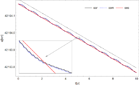
Figure 1: Comparison of Cartesian equations including the 2-body problem and PR/SW-drag (black-thick), complete Gaussian (blue-dotted), and secular (red-thick) model. Black, dashed: slope of the drift based on the analytical estimate (12). Lower left: magnification of the central part of the figure.

3.2 Equilibria and linear stability analysis

To highlight the role of solar radiation pressure and PR/SW-drag on the location of the equilibrium of the geostationary orbit we make use of a simplified system of equations that qualitatively describes the motion of the SDO close to the geostationary orbit, i.e. close to the 1:1 resonance between the orbital period of the SDO and the rotational period of the Earth. First, we omit the gravitational effect of the Sun and the Moon on the motion of the SDO, and just take the gravitational field of the Earth up to degree and order $2$, solar radiation pressure, and the combined PR/SW-drag terms of (1) into account. Next, we derive the components $da/dt$, $dM/dt$ of (6) that are needed to get the components $dL/dt$, $dl/dt$ of (2.3) for both, the gravitational field of the Earth, $V_{E}$, and the solar radiation pressure term $V_{SRP}$. Let $\tilde{\omega}=\omega+\Omega$, and again let $\theta$ be the Greenwich Meridian angle. We introduce the resonant argument for the stationary orbit as

$$\lambda=M-\theta+\tilde{\omega}\ .$$

Next we insert $\lambda$ into the expression for $dL/dt$, $dl/dt$ in (2.3) and average over the rotation period $\theta$. Let $\mathfrak{H}_{res}$, $\mathfrak{f}_{L,res}$, $\mathfrak{f}_{l,res}$ denote the resulting averaged terms. The equilibrium that defines the stationary orbit in this simplified resonant system is provided by the set of equations:

$$\frac{dL}{dt}=-\frac{d\mathfrak{H}_{res}}{d\lambda}+{\mathfrak{f}}_{L,res}=0\ ,\quad\frac{d\lambda}{dt}=\frac{d\mathfrak{H}_{res}}{dL}+{\mathfrak{f}}_{l,res}=0\ ,$$ (15)

where the last relation holds up to a constant and where we assumed that $d\tilde{\omega}/dt$ is zero. We remark that in equations (15) the terms in $\mathfrak{H}_{res}$ are stemming from $V_{E}$, $V_{SRP}$, while the terms in $\mathfrak{f}_{L,res}$, $\mathfrak{f}_{l,res}$ originate from $\vec{F}_{PR/SW}$ in (1). Since (15) still depends on all Keplerian elements, we fix all but $a$, $\lambda$, for which we solve for given system parameters. We present our results in the ($\Delta a,\Delta\lambda)$ -plane, where $\Delta a=a_{c}-a_{*}$, $\Delta\lambda=\lambda_{c}-\lambda_{*}$ with $a_{c}$, $\lambda_{c}$ being the solution of the classical problem (i.e., without PR/SW-drag), and $a_{*}$, $\lambda_{*}$ are the values that solve (15) including the PR/SW-drag. Our results are summarized in Figure 2. We clearly see that solar radiation pressure and the drag terms together shift the location of the geostationary equilibrium up to $50\ mt$ in semi-major axis, and up to $6{}^{o}$ in orbital longitude. If we neglect the drag terms, but still take into account the solar radiation pressure terms, the shift in semi-major axis persists. Therefore, we conclude, that the shift in semi-major axis is mainly caused by the effect of solar radiation pressure alone, while the shift in orbital longitude is necessary to balance the additional effect of the drag terms. Figure 2 also shows that for the parameter values used in the figure, the role of solar wind is not negligible for high area-to-mass ratios.

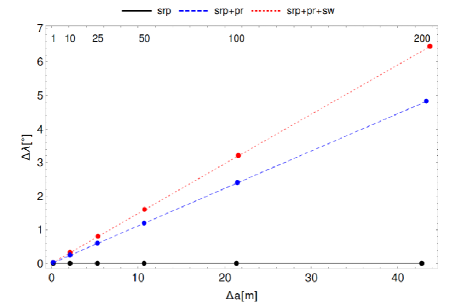
Figure 2: Location of the equilibria in the $(\Delta a,\Delta\lambda)$-plane for $A/m=1$, 10, 25, 50, 100, 200 (small ticks): solar radiation pressure alone (black, thick), with the additional Poynting-Robertson effect (blue, dashed), all together with solar wind drag (red, dotted), i.e. $\eta=1/3$, $Q=1$. Additional Kepler elements have been set to $e=0$, $i=0{}^{o}$, $\omega=0{}^{o}$, $\Omega=0{}^{o}$, respectively.

Next, we linearize the left hand sides of (15) around the stationary solution, and calculate the eigenvalues $(\zeta_{1},\zeta_{2})$ of the linearized system for the same parameters and initial conditions as in the study of the equilibria. Our results are provided in Figure 3: we clearly see, that the combined PR/SW-drag effect introduces a positive real part to $(\zeta_{1},\zeta_{2})$ growing with increasing $A/m$ ratio. For comparison, we also derive the eigenvalues on the basis of $V_{E}$, as well as of $V_{E}$ and $V_{SRP}$ in (15). In both cases, the eigenvalues stay complex, yielding the elliptic character of the equilibrium for circular orbits.

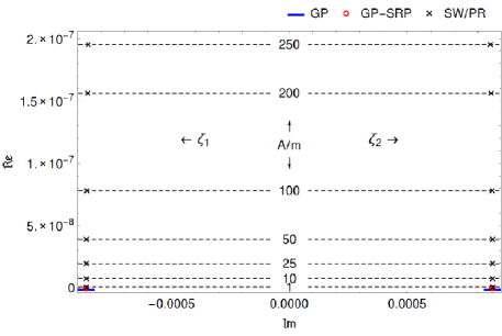
Figure 3: Eigenvalues, in the $({\mathfrak{I}m},{\mathfrak{R}e})$-plane, of the linearized system of (15) expanded around the stationary point for different $A/m$ (indicated by small numbers inside the plot), for the same circular orbit as in Figure 2.

To conclude, let us mention that in the following we will refer to a GEO 1:1 resonance, whenever the following relation holds:

$$\dot{M}-\dot{\theta}=0\ ,$$

where $\dot{M}$ corresponds to the mean motion of the SDO, while $\dot{\theta}$ denotes the angular speed of rotation of the Earth. Such resonance corresponds to a geostationary orbit located on the equatorial plane at a distance of about 42 164.17 $km$ from the center of the Earth.

4 Temporary trapping or escape from the resonance

In this section we perform several numerical experiments to study the behavior of the orbits close to the GEO 1:1 resonance. As it is well known, within the conservative framework the GEO 1:1 resonance shows a pendulum-like phase portrait. Indeed, the exact 1:1 resonance corresponds to the equilibrium point, which is surrounded by a librational island, whose border is delimited by a chaotic separatrix (Celletti & Galeş (2014)). When the dissipation is switched on, the orbits might collapse on the equilibrium, can be temporarily trapped in a resonant regime, or rather escape from the resonance (Neĭshtadt (2005)). Although the PR-SW drag is rather weak, we observe that its effect is not negligible on a proper time scale, as shown in the Sections 4.1 and 4.2.

Let us premise some information about the parameters and data used in the forthcoming numerical simulations: the astronomical constants ${\mathcal{G}}m_{E}$, ${\mathcal{G}}m_{M}$, $Gm_{S}$ are taken from Luzum et al. (2011), the gravity field of the Earth (tide-free gravity field EGM2008) are obtained from Pavlis (2013); Pavlis et al. (2012). The ranges for various parameters related to PR/SW-drag are derived on the basis of values found in the literature (see Burns et al. (1979); Gustafson (1994); Kocifaj et al. (2006)). We remark that for typical optical properties and densities, that are consistent with observations, $\beta\simeq 0.2/s$ (with the radius $s$ of a spherical particle given in $[\mu mt]$, see, e.g. Beaugé & Ferraz-Mello (1994)), or $\beta\simeq 7.6\times 10^{-4}A/m$ (with $A/m$ given in $[mt^{2}/kg]$, see, e.g. Kocifaj et al. (2006)) may be used.

In all numerical simulations, the initial Epoch is J2000 (January 1, 2000, 12:00 GMT). We provide the numerical results in terms of osculating orbital elements. The transformation between inertial Cartesian coordinates and osculating Kepler elements is summarized in Appendix A.

4.1 Drift motion (outside resonances)

Outside a resonant regime, the dynamical behavior leads to a drift of the semimajor axis. This is well explained by the following example of drift motion, which is shown in Figure 4, obtained by a direct numerical integration of (1) (including all effects). The drift in semimajor axis is conveniently described by the secular theory developed in Section 3, i.e. formula (12).

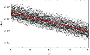
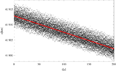
Figure 4: Typical drift motion in semi-major axis $a$ outside a resonant regime. Parameters and osculating initial conditions are: $A/m=1\,[mt^{2}/kg]$, $a(0)=41914.1696\ [km]$, $e(0)=0.2$, $i(0)=0{}^{o}$, $\omega(0)=0{}^{o}$, $\Omega(0)=0{}^{o}$, $M(0)=0{}^{o}$. Left: $\eta=0$ (without solar wind). Right: $\eta=1/3$, $Q=1$ (with solar wind). The slope of the drift rate calculated on the basis of (12) is shown in red-thick.

We provide a survey of the drift rates in Figure 5: while in the rotational regime of motion of the resonant angle $\lambda$, the drift due to the combined PR/SW-effect is essentially described by a constant linear drift, the drift rates are spread, when getting close to the exact resonance. Figure 5 also shows that the role of Moon and Sun becomes relevant outside the resonance, as already noticed, e.g., in Celletti & Galeş (2015), Rosengren et al. (2015).

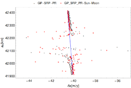
Figure 5: Drift rates close to the GEO regime of motion. Numerically obtained drift rates on the basis of (1) for osculating initial conditions within $a(0)=a_{0}$ and $41914.1696\ [km]\leq a_{0}\leq 42414.1696\ [km]$, and same parameters and additional initial conditions as in Figure 4. Black-cross: without the additional effect of the Sun and the Moon. Red-circle: full model. Blue-thick line: drift rates calculated on the basis of (12).

4.2 Behavior in the neighborhood of the GEO 1:1 resonance

Depending on parameters and initial conditions, the numerical study unveils a rich dynamical behavior in the vicinity of the 1:1 resonance, much more complex than the linear drift described above, consisting of trapped motions in primary or higher order resonances, resonance captures, escapes from resonance and jumps. Although we know that such behavior is typical of dissipative systems, we aim to show that PR-SW drag is not negligible on reasonably long time scales. For instance, Figure 7, upper plots, will show the stabilizing effect of the resonance condition between the orbital period of the satellite and the rotational period of the Earth on the long-term motion of the SDO (temporarily trapped motion into primary resonance). We clearly see that initial conditions starting in the librational regime of motion of the resonant angle $\lambda$ stay close to their initial orbital semi-major axis $a(0)$ on long time scales.

In order to point out the role of the PR–drag effect close to the 1:1 resonance and to depict numerically all the above mentioned phenomena, we consider two sample objects having $A/m=1\,[mt^{2}/kg]$ and $A/m=15\,[mt^{2}/kg]$, respectively. For spherical bodies having the typical density $\rho=2.2\,[g/cm^{3}]$, these values of the area-to-mass ratio correspond to debris of the order of sub-millimeters in diameter.

To avoid complex effects induced by the lunisolar secular resonances (see for example Hughes (1980); Celletti et al. (2016); Daquin et al. (2016)), we focus on a region of the space of orbital elements characterized by small inclinations and not very large eccentricities, where instead lunisolar secular resonances might strongly influence the dynamics. As a matter of fact, in computations, we took the initial inclination $i(0)=10^{o}$ and the initial eccentricity $e(0)=0.2$. Since the eccentricity is not zero, for large values of the area-to-mass ratio, like $A/m=15\,[mt^{2}/kg]$, some secondary resonances between the geostationary libration angle $\lambda$ and the Sun’s longitude, denoted hereafter by $\lambda_{Sun}$, appear as effect of the solar radiation pressure (Valk et al. (2009); Lemaître et al. (2009)). We remark that the term secondary is commonly used to describes resonances within a librational regime, while here - in agreement with the terminology adopted in Valk et al. (2009) - we label secondary those resonances which are due to an interaction between the geostationary libration angle and the longitude of the Sun.

To highlight the influence of the PR/SW drag, it is important to discuss first the dynamical effect induced by the other perturbations (namely, by the conservative part), in particular the solar radiation pressure. Figure 6 computes two FLI plots for the Cartesian model described in Section 2.1, which includes all perturbations but PR/SW–drag effect, when the area to mass ratio parameter has the values $A/m=1\,[mt^{2}/kg]$ (left panel) and $A/m=15\,[mt^{2}/kg]$ (right panel). The (osculating) initial conditions are $e(0)=0.2$, $i(0)=10^{o}$, $\omega(0)=10^{o}$, $\Omega(0)=20^{o}$. The color scale provides a measure of the FLI, which gives an indication of the regular or chaotic dynamics: small values (i.e., dark colors) correspond to regular motions, while larger values (i.e., red to yellow colors) denote chaotic regions. The phase plane $\lambda$–$a$ is very similar to that of a pendulum for $A/m=1\,[mt^{2}/kg]$ (left panel of Figure 6). The semimajor axis $a$ and the resonant angle $\lambda$ librate or circulate; the red-yellow curves divide the phase space in regions corresponding to libration or circulation.

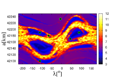
Figure 6: FLI map (using Cartesian equations) for the GEO 1:1 resonance, under the effect of the following perturbations: solar radiation pressure, Earth’s harmonics up to $n=m=3$, Sun and Moon (conservative case). The osculating initial conditions are: $e(0)=0.2$, $i(0)=10^{o}$, $\omega(0)=10^{o}$, $\Omega(0)=20^{o}$. Left: $A/m=1\,[mt^{2}/kg]$; Right: $A/m=15\,[mt^{2}/kg]$. The green–black circles represent the orbits analyzed in Figures 7, 8, 9, 10 and 11, in the framework of the full model which includes also the PR/SW–drag effect.

However, when the area-to-mass ratio parameter is larger, say $A/m=15\,[mt^{2}/kg]$, then besides the libration region associated to the primary resonance $\dot{\lambda}=0$, some new structures are visible in the right panel of Figure 6, which account for some secondary resonances involving a linear combination of the geostationary resonant angle $\lambda$ with the longitude of the Sun $\lambda_{Sun}$ (see Valk et al. (2009); Lemaître et al. (2009); Celletti & Galeş (2015) for a detailed description of the web of secondary resonances appearing outside the geostationary resonance as a product of the interaction of solar radiation pressure with different tesseral resonances). In fact, as Figures 8, 9 and 11 infer, the six larger libration islands visible in the right panel of Figure 6 are due to the following resonances: $\dot{\lambda}+{1\over 2}\dot{\lambda}_{Sun}=0$ (the two blue regions located on top of the plot), $\dot{\lambda}=0$ (the two largest islands) and $\dot{\lambda}-{1\over 2}\dot{\lambda}_{Sun}=0$ (the regions located at the bottom of the plot). The chaotic region that surrounds the libration islands is due to the interaction of these three resonances.

Comparing the patterns shown in the two panels of Figure 6, we notice that a larger area-to-mass ratio, say $A/m=15\,[mt^{2}/kg]$ (right plot), strongly deforms the phase space plots, as a result of the influence of the short periodic part of the disturbing forces, in particular as an effect of the action of the solar radiation pressure. Each disturbing force, namely the oblateness of the Earth, the attraction of the Moon and of the Sun, and the solar radiation pressure, induces a short periodic variation of the orbital elements. These elements, used in the framework of the Cartesian formulation and called osculating orbital elements, differ from the mean orbital elements used in the secular theories. For perturbations relatively small in magnitude, the difference between the mean and osculating elements is not so evident. However, for large perturbations, like that due to the effect of solar radiation pressure when $A/m=15\,[mt^{2}/kg]$, there is a remarkable difference between the osculating and mean elements. However, we underline that in the rest of this section we deal with the osculating orbital elements.

Within the conservative dynamical background described above, let us now consider the dissipative effects induced by the PR/SW–drag. By merging the results given by the secular theory with numerical investigations, in the following we describe the weak influence of PR/SW drag and exemplify with some concrete examples the complex dynamical behavior near the GEO 1:1 resonance on large time scales.

Let us recall first that the stability analysis presented in Section 3.2 shows that the equilibria of the simplified resonant dissipative system (15) are repellors. So, as theories of dynamical systems suggest, the initial conditions located in the vicinity of these points do not evolve toward but rather away from them. Thus, within the framework of the dissipative system, the libration regions in Figure 6 should become a sort of “basins of repulsion”. However, as Figure 3 shows, the positive real parts of the eigenvalues $(\zeta_{1},\zeta_{2})$ of the linearized system are very small in comparison with the absolute values of the imaginary parts. Therefore, in numerical investigations we expect this effect to be very small even on long time scales. Because the PR/SW-drag effect is weak, we will still use the terminology “libration regions”, even in the case of the full (dissipative) model, and not “basins of repulsion” as we should normally adopt in the framework of dissipative dynamical systems.

In Figures 7, 8, 9, 10 and 11 we report some results obtained by propagating several osculating initial conditions for a time reaching at most 1000 years, starting from January 1.5, 2000 (J2000). All these orbits are represented by green–black circles in Figure 6, which provided a picture within the conservative case.

The combined influence of the dissipative effects (the fact that equilibrium points are repellors) and of the conservative part can lead to escape motions after a transient time, as shown by the top panels of Figure 7 for $A/m=1\,[mt^{2}/kg]$, and the top panels of Figure 8 for $A/m=15\,[mt^{2}/kg]$. However, the initial condition should be close enough to the separatrix for $A/m=1\,[mt^{2}/kg]$, or sufficiently near the chaotic region for $A/m=15\,[mt^{2}/kg]$ (see Figure 6). Besides, the escape time is very large, more than 900 years in the case of the orbit analysed in the top panels of Figure 7 for $A/m=1\,[mt^{2}/kg]$. These initial conditions lead to an escape orbit; however, our tests show that a small change in initial conditions, for example in $\lambda$, from $\lambda(0)=5^{o}$ to $\lambda(0)=6^{o}$, leads to a trapped motion for more than 1000 years. In addition, we find drift, temporary capture and release from resonance for $\lambda=20{}^{o}$ (middle panels of Figure 7), but also drift and long-term capture (bottom panels of Figure 7) for $\lambda=0{}^{o}$.

For larger area-to-mass ratios, the effects induced by both the solar radiation pressure and PR/SW–drag increase in intensity. Figure 8, top panels, obtained for $A/m=15\,[mt^{2}/kg]$, show an escape orbit characterized by a smaller escape time; due to large perturbations, it crosses multiple dynamical regimes (temporary escapes and captures), before it escapes definitively at about 310 years. In fact, as the numerical results are showing, the escape time depends on multiple factors: parameters, how close the initial conditions are from the separatrix (or from the chaotic region), the magnitude of the perturbing forces, the interaction between various perturbations.

For $A/m=15\,[mt^{2}/kg]$, given the fact that the dynamical background is much more complex than for relatively small area-to-mass ratios, the matter is a little bit more complicated. The orbit described by the top plots of Figure 8, and which is located in the libration region of the primary resonance (compare with the right panel of Figure 6), is an escape orbit. This does not mean that any orbit located in libration regions is an escape orbit. As discussed above, it depends on how close the initial condition is from the equilibrium point located inside the libration region. For example, the bottom plots of Figure 8 describe a temporarily trapped motion into a primary resonance. It is interesting to point out that trapped motions exist also into the secondary resonances $\dot{\lambda}+{1\over 2}\dot{\lambda}_{Sun}=0$ and $\dot{\lambda}-{1\over 2}\dot{\lambda}_{Sun}=0$, as shown in Figure 9.

In order to have a holistic picture of the dynamics for $A/m=15\,[mt^{2}/kg]$, inside the GEO 1:1 resonance, we should describe the behavior of the orbits located in the chaotic region. Since the interaction between the primary resonance and the secondary resonances is large, an initial condition from the chaotic region leads to an escape orbit on a scale of time of the order of tens (at most two hundred) years. To reveal the complex interplay between resonances and PR/SW–drag effect, in Figure 10 and 11 we represent the evolution of the semimajor axis $a$, and the resonant angles $\lambda+\lambda_{Sun}/2$, $\lambda$ and $\lambda-\lambda_{Sun}/2$, associated to each resonance. As Figures 10 and 11 show, the orbit is affected by all resonances, since there is a temporary trapping in each resonance at different intervals of time. The escape time is less than 100 years.

Finally, to completely describe the behavior in the near vicinity of the GEO 1:1 resonance, one should understand the behavior of the orbits located initially at a longer distance than that at which the resonance pattern is located. As effect of the interaction between the dissipative and conservative parts of the perturbations, numerical simulations show that there are possible jumps, usually for small area-to-mass ratios (not shown here), temporary captures into the primary resonance (middle panels of Figure 7), temporary captures into primary and secondary resonance (Figures 10 and 11) or even captures for times longer than 1000 years (bottom panels of Figure 7). It is important to note that in either of the cases, capture into primary resonance or capture into secondary resonances, the orbit does not approach toward the center of libration island, but rather remains on a long time scale in a very close neighborhood of the separatrix.

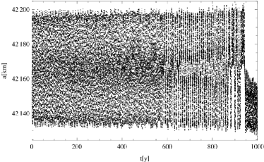
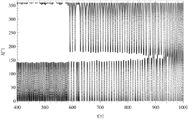
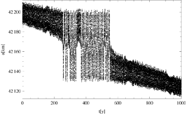
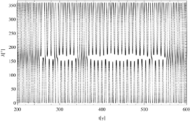
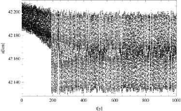
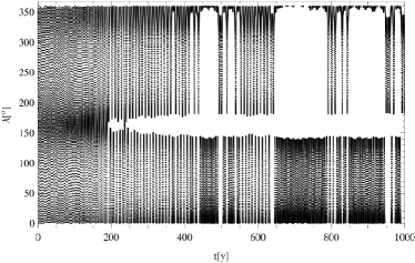
Figure 7: Variation of the semimajor axis $a$ and resonant angle $\lambda$ for three orbits located in the neighborhood of the 1:1 resonance. Parameters and osculating initial conditions are $A/m=1\ [mt^{2}/kg]$, $\eta=0$, $i(0)=10^{o}$, $e=0.2$, $\omega(0)=10^{o}$, $\Omega(0)=20^{o}$ and: $a(0)=42164\,km$, $\lambda(0)=5^{o}$ (or $M(0)=-25^{o}$) (top panels); $a(0)=42198\,km$, $\lambda(0)=20^{o}$ (or $M(0)=-10^{o}$) (middle panels); $a(0)=42190\,km$, $\lambda(0)=0^{o}$ (or $M(0)=-30^{o}$) (bottom panels). Compare with the left panel of Figure 6.

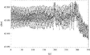
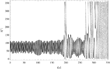
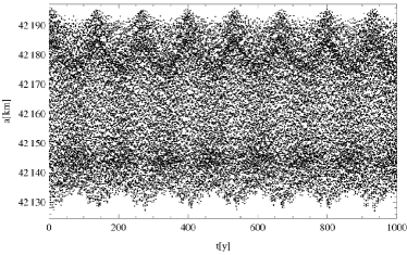
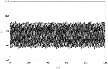
Figure 8: Escape motion from the primary resonance (top) and trapped motion into primary resonance (bottom). Variation of the semimajor axis $a$ and the resonant angle $\lambda$ for two orbits in the libration region of primary resonance. Parameters and osculating initial conditions are $A/m=15\ [mt^{2}/kg]$, $\eta=0$, $i(0)=10^{o}$, $e=0.2$, $\omega(0)=10^{o}$, $\Omega(0)=20^{o}$ and: $a(0)=42170\,km$, $\lambda(0)=45^{o}$ (or $M(0)=15^{o}$) (upper panels); $a(0)=42190\,km$, $\lambda(0)=90^{o}$ (or $M(0)=60^{o}$) (bottom panels). Compare with the right panel of Figure 6.

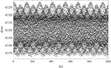
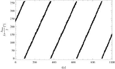
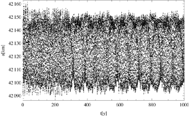
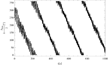
Figure 9: Trapped motions into secondary resonances $\dot{\lambda}+\frac{\dot{\lambda}_{Sun}}{2}=0$ (top) and $\dot{\lambda}-\frac{\dot{\lambda}_{Sun}}{2}=0$ (bottom). Variation of the semimajor axis $a$ and the resonant angle $\lambda+\lambda_{Sun}/2$ (top) and $\lambda-\lambda_{Sun}/2$ (bottom) for two orbits trapped in the secondary resonances $\dot{\lambda}+\frac{\dot{\lambda}_{Sun}}{2}=0$ (top) and $\dot{\lambda}-\frac{\dot{\lambda}_{Sun}}{2}=0$ (bottom). Parameters and osculating initial conditions are $A/m=15\ [mt^{2}/kg]$, $\eta=0$, $i(0)=10^{o}$, $e=0.2$, $\omega(0)=10^{o}$, $\Omega(0)=20^{o}$ and: $a(0)=42190\,km$, $\lambda(0)=-130^{o}$ (or $M(0)=-160^{o}$) (upper panels); $a(0)=42100\,km$, $\lambda(0)=-110^{o}$ (or $M(0)=-140^{o}$) (bottom panels). Compare with the right panel of Figure 6.

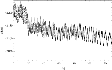
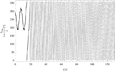
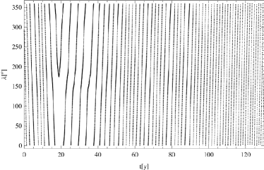
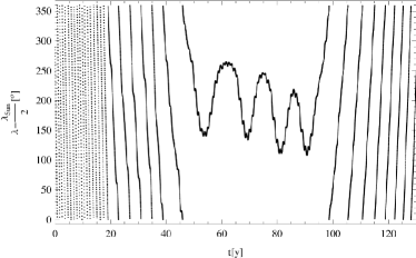
Figure 10: Initial conditions are taken within the chaotic region surrounding the GEO 1:1 resonance. Variation of the semimajor axis $a$ (top left) and the angles $\lambda+\lambda_{Sun}/2$ (top right), $\lambda$ (bottom left), $\lambda-\lambda_{Sun}/2$ (bottom right) for an orbit having the following parameters and osculating initial conditions: $A/m=15\ [mt^{2}/kg]$, $\eta=0$, $i(0)=10^{o}$, $e=0.2$, $\omega(0)=10^{o}$, $\Omega(0)=20^{o}$, $a(0)=42178\,km$ and $\lambda(0)=-50^{o}$ (or $M(0)=-80^{o}$). Compare with the right panel of Figure 6.

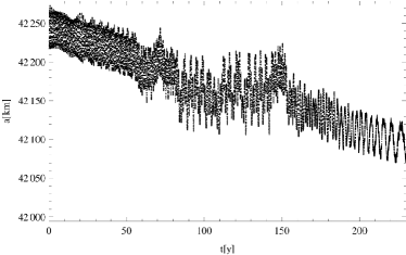
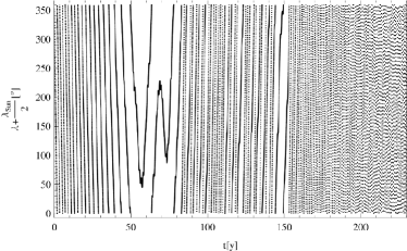
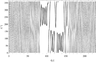
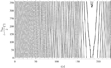
Figure 11: Initial conditions are taken outside (above) the GEO 1:1 resonance. Variation of the semimajor axis $a$ (top left) and the angles $\lambda+\lambda_{Sun}/2$ (top right), $\lambda$ (bottom left), $\lambda-\lambda_{Sun}/2$ (bottom right) for an orbit having the following parameters and osculating initial conditions: $A/m=15\ [mt^{2}/kg]$, $\eta=0$, $i(0)=10^{o}$, $e=0.2$, $\omega(0)=10^{o}$, $\Omega(0)=20^{o}$, $a(0)=42233\,km$ and $\lambda(0)=-5^{o}$ (or $M(0)=-35^{o}$). Compare with the right panel of Figure 6.

As a final experiment, we perform a numerical integration of the equations of motion with and without PR effect. Figure 12 shows the difference in orbital elements $(a,e,i)$ over 100 and 1000 years. The longer is the timescale, the stronger is the influence of the PR effect. We also computed several other integrations, all showing that PR effect is not so relevant for small values of the initial eccentricity, as well as for small values of the area-to-mass ratio.

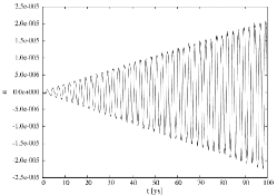
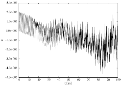
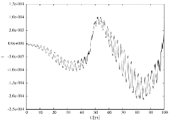
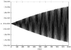
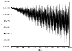
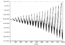
Figure 12: Difference of the integration with and without Poynting–Robertson effect. The other effects included in the equations of motion are: Earth’s harmonics up to $n=m=3$, SRP, Sun and Moon. Here we take $a=42164.8$ km, $e=0.1$, $i=3^{o}$, $\omega=5^{o}$, $\Omega=10^{o}$, $M=20^{o}$, $A/m=1\ [mt^{2}/kg]$. The left panels refer to the semimajor axis (in units of $a_{geo}\equiv 42\,164.17\ [km]$, the middle panels to the eccentricity, the right panels to the inclination (in degrees). The upper panels show the integration over 100 years, while the lower panels over 1000 years.

5 Conclusions

It is well known that Poynting-Robertson and solar wind drag contribute as dissipative effects acting over long time scales on artificial satellites and space debris. We explore the behavior of the dynamics in the vicinity of the GEO 1:1 resonance for two sample objects characterized by $A/m=1\,[mt^{2}/kg]$ and $A/m=15\,[mt^{2}/kg]$. Given the fact that the population of objects in the GEO region continues to grow, it is important to know how small objects (equivalently, large objects having high area-to-mass ratios), which could result from a catastrophic event, behave under the combined effect of dissipative forces and conservative perturbations. Understanding their dynamics is crucial for risk evaluation and mitigation strategies.

Although several studies were performed in the past years to evaluate the role of the dissipative effects due to PR/SW, we are not aware of any investigation of PR/SW drag combined with a careful analysis of the dynamical properties of the phase space. We know that equilibria are repellors both within and outside the librational region, but the evolution of a space debris strongly depends on its initial location as well as its area-to-mass ratio. Indeed, the study performed in the previous sections show that a debris with relatively small area-to-mass ratio, say $A/m=1\ [mt^{2}/kg]$, might undergo different behaviors, even when changing a little the initial conditions. The three case studies considered in Figure 6, left panel, show that, although being all close to the separatrix, the debris can be trapped into resonance for a long time and then escape (Figure 7, top panels), or rather it can be only temporary trapped (Figure 7, middle panels), or trapped after a transient time (Figure 7, bottom panels).

On the other hand, when the area-to-mass ratio is large, say $A/m=15\ [mt^{2}/kg]$, the structure of the phase space changes significantly: chaotic motions occupy a relevant portion of the phase space, while secondary resonances make their appearance, thus reflecting the interaction with the longitude of the Sun (see Figure 6, right panel).

The investigation given in this work leads to a zoo of dynamical behaviors under PR/SW drag: temporary trapping or escape from the primary resonance, temporary trapping or escape from one of the secondary resonances. All these information can be conveniently used to monitor the long-term behavior of space debris, and in particular can be used to evaluate the decay rate due to PR/SW drag. Since the dynamical behavior is very sensitive to small displacements of the object in the phase space, one could even design a strategy which exploits PR/SW drag to move space debris within different regions for the safeguard of operational satellites.

Appendix A

Gravity field

The quantities $P_{nm}$ in (1) are defined in terms of the standard Legendre polynomials:

$$P_{n}(x)\equiv{1\over{2^{n}n!}}\ {{d^{n}}\over{dx^{n}}}\{(x^{2}-1)^{n}\}\ ,\qquad P_{nm}(x)\equiv(1-x^{2})^{m\over 2}\ {{d^{m}}\over{dx^{m}}}\{P_{n}(x)\}\ .$$

The coefficients $C_{nm}$, $S_{nm}$ are defined as

$$C_{nm} \equiv {{2-\delta_{0m}}\over m_{E}}\ {{(n-m)!}\over{(n+m)!}}\ \int_{V_{E}}({r_{p}\over R_{E}})^{n}\ P_{nm}(\sin\phi_{p})\ \cos(m\lambda_{p})\delta(\underline{r}_{p})\ dV_{E}$$

$$S_{nm} \equiv {{2-\delta_{0m}}\over m_{E}}\ {{(n-m)!}\over{(n+m)!}}\ \int_{V_{E}}({r_{p}\over R_{E}})^{n}\ P_{nm}(\sin\phi_{p})\ \sin(m\lambda_{p})\delta(\underline{r}_{p})\ dV_{E}\ ,$$

where $(r_{p},\lambda_{p},\phi_{p})$ are the spherical coordinates of some point $P$ inside the Earth ($\delta_{jm}$ is the Kronecker symbol).

Rotation matrices

The rotation matrices are defined as follows:

$${\mathfrak{R}}_{1}(\varphi)=\left(\begin{array}[]{ccc}1&0&0\\ 0&\cos\varphi&-\sin\varphi\\ 0&\sin\varphi&\cos\varphi\\ \end{array}\right)\ ,\quad{\mathfrak{R}}_{3}(\varphi)=\left(\begin{array}[]{ccc}\cos\varphi&-\sin\varphi&0\\ \sin\varphi&\cos\varphi&0\\ 0&0&1\\ \end{array}\right)\ .$$

Osculating orbital elements

The orbital elements $a$, $e$, $i$, $\omega$, $\Omega$, $M$ are obtained from the Cartesian position $\vec{r}$ and velocity $\vec{v}$ by means of the following procedure. Let $\mu={\mathcal{G}}m_{E}$ and $\vec{I}=(1,0,0)$, $\vec{J}=(0,1,0)$, $\vec{K}=(0,0,1)$. Furthermore, $r=|\vec{r}|$, $v=|\vec{v}|$ and let $h\vec{K}=\vec{r}\wedge\vec{v}$ be the angular momentum with $h=|\vec{h}|$. From the eccentricity vector

$$\vec{e}={{\vec{v}\wedge\vec{h}}\over{\mu}}-{{\vec{r}}\over{r}}$$

we calculate the eccentricity $e=|\underline{e}|$. The semi-major axis is obtained by the relation

$$h^{2}=\mu a(1-e^{2})\ ,$$

while the inclination can be obtained from

$$\cos i={{\vec{h}\cdot\vec{K}}\over{h}}\ .$$

Let $\vec{n}/n$ be the unit nodal vector with $\vec{n}=\vec{K}\wedge\vec{h}$ and $n=|\vec{n}|$; then, $\Omega$ is given by

$$\cos\Omega={\vec{n}\cdot\vec{I}\over n}\ ,\qquad\sin\Omega={\vec{n}\cdot\vec{J}\over n}\ .$$

The argument of perigee is obtained from

$$\cos\omega={\vec{n}\cdot\vec{e}\over{ne}}\ ,\qquad\sin\omega=({\vec{n}\over n}\wedge{\vec{e}\over e})\cdot{\vec{h}\over h}\ .$$

The true anomaly $f$ is given by

$$\cos f={{\vec{e}\cdot\vec{r}}\over{e\,r}}\ ,$$

while the eccentric anomaly is obtained from

$$\cos E={{e+\cos f}\over{1+e\cos f}}\ ,$$

which, together with Kepler’s equation

$$M=E-e\sin E\ ,$$

provides the mean anomaly $M$.

References

- Beaugé & Ferraz-Mello (1994) Beaugé C., Ferraz-Mello S., 1994, Icarus, 110, 239
- Burns et al. (1979) Burns J. A., Lamy P. L., Soter S., 1979, Icarus, 40, 1
- Celletti & Galeş (2015) Celletti A., Galeş C., 2015, Advances in Space Research, 56, 388
- Celletti et al. (2016) Celletti A., Galeş C., Pucacco G., Rosengren A., 2016, Preprint
- Celletti & Galeş (2014) Celletti A., Galeş C., 2014, J. Nonlinear Sci., 24, 1231
- Celletti & Galeş (2015) Celletti A., Galeş C., 2015, Adv. Spac. Res., 56, 388
- Celletti & Lhotka (2012) Celletti A., Lhotka C., 2012, Regular and Chaotic Dynamics, 17, 273
- Daquin et al. (2016) Daquin J., Rosengren A. J., Alessi E. M., Deleflie F., Valsecchi G. B., Rossi A., 2016, Celestial Mechanics and Dynamical Astronomy, 124, 335
- Dvorak & Lhotka (2013) Dvorak R., Lhotka C., 2013, Celestial Dynamics: Chaoticity and Dynamics of Celestial Systems. Wiley-VCH
- Fitzpatrick (1970) Fitzpatrick P. M., 1970, Principles of celestial mechanics. Academic Press, New York
- Froeschlé et al. (1997) Froeschlé C., Lega E., Gonczi R., 1997, Celestial Mechanics and Dynamical Astronomy, 67, 41
- Früh & Schildknecht (2012) Früh C., Schildknecht T., 2012, MNRAS, 419, 3521
- Gustafson (1994) Gustafson B. A. S., 1994, Annual Review of Earth and Planetary Sciences, 22, 553
- Hubaux & Lemaître (2013) Hubaux C., Lemaître A., 2013, Celestial Mechanics and Dynamical Astronomy, 116, 79
- Hughes (1980) Hughes S., 1980, Proceedings of the Royal Society of London Series A, 372, 243
- Klačka (2014) Klačka J., 2014, MNRAS, 443, 213
- Kocifaj et al. (2006) Kocifaj M., Klačka J., Horvath H., 2006, MNRAS, 370, 1876
- Kuznetsov & Zakharova (2015) Kuznetsov E., Zakharova P., 2015, Advances in Space Research, 56, 406
- Kuznetsov (2011) Kuznetsov E. D., 2011, Solar System Research, 45, 433
- Kuznetsov et al. (2013) Kuznetsov E. D., Zakharova P. E., Glamazda D. V., Kudryavtsev S. O., 2013, in 6th European Conference on Space Debris Vol. 723 of ESA Special Publication, Light Pressure Effect on the Orbital Evolution of Space Debris in Low-Order Resonance Regions. p. 157
- Kuznetsov et al. (2014) Kuznetsov E. D., Zakharova P. E., Glamazda D. V., Kudryavtsev S. O., 2014, Solar System Research, 48, 446
- Kuznetsov et al. (2012) Kuznetsov E. D., Zakharova P. E., Glamazda D. V., Shagabutdinov A. I., Kudryavtsev S. O., 2012, Solar System Research, 46, 442
- Lemaître et al. (2009) Lemaître A., Delsate N., Valk S., 2009, Celestial Mechanics and Dynamical Astronomy, 104, 383
- Lhotka & Celletti (2013) Lhotka C., Celletti A., 2013, International Journal of Bifurcation and Chaos, 23, 50036
- Lhotka & Celletti (2015) Lhotka C., Celletti A., 2015, Icarus, 250, 249
- Luzum et al. (2011) Luzum B., Capitaine N., Fienga A., Folkner W., Fukushima T., Hilton J., Hohenkerk C., Krasinsky G., Petit G., Pitjeva E., Soffel M., Wallace P., 2011, Celestial Mechanics and Dynamical Astronomy, 110, 293
- McMahon & Scheeres (2010) McMahon J., Scheeres D., 2010, Celestial Mechanics and Dynamical Astronomy, 106, 261
- Montenbruck & Gill (2000) Montenbruck O., Gill E., 2000, Satellite Orbits: Models, Methods, and Applications. Physics and astronomy online library, Springer Berlin Heidelberg
- Moulton (1914) Moulton F. R., 1914, An Introduction to Celestial Mechanics. The MacMillan Company, New York
- Murray & Dermott (1999) Murray C., Dermott S., 1999, Solar System Dynamics. Cambridge University Press
- Neĭshtadt (2005) Neĭshtadt A. I., 2005, Tr. Mat. Inst. Steklova, 250, 198
-
Pavlis (2013)
Pavlis N., , 2013, Earth Gravitational Model 2008 (EGM2008),
http://earth-info.nga.mil/GandG/wgs84/gravitymod/egm2008/ - Pavlis et al. (2012) Pavlis N., Holmes S., Kenyon S., Factor J., 2012, JGR, 117, B04406
- Rosengren et al. (2015) Rosengren A. J., Alessi E. M., Rossi A., Valsecchi G. B., 2015, MNRAS, 449, 3522
- Slabinski (1980) Slabinski V. J., 1980, in Bulletin of the American Astronomical Society Vol. 12, Poynting-Robertson drag on satellites near synchronous altitude. p. 741
- Slabinski (1983) Slabinski V. J., 1983, in Bulletin of the American Astronomical Society Vol. 15, Poynting-Robertson force allowing for wavelength-dependent reflection coefficients and non-spherical shapes. p. 869
- Smirnov & Mikisha (1993) Smirnov M., Mikisha A., 1993, in The Technogeneous Space Debris Problems Secular Evolution of Geostationary Objects Caused by Light Pressure. pp 126–142
- Smirnov & Mikisha (1995) Smirnov M., Mikisha A., 1995, in Collisions in the Surrounding Space (Space Debris) Secular Evolution of Space Bodies on High Orbits due to Light Pressure. Part II. pp 252–271
- Tueva & Avdyushev (2006) Tueva O., Avdyushev V., 2006, in Sbornik trudov konf. Okolozemnaya astronomiya-2005 How the Light Pressure and Poynting-Robertson Effect Influence onto Space Debris Dynamic. pp 261–267
- Valk et al. (2009) Valk S., Delsate N., Lemaître A., Carletti T., 2009, Advances in Space Research, 43, 1509