A Rapid Pattern-Recognition Method for Driving Styles Using Clustering-Based Support Vector Machines
Abstract
A rapid pattern-recognition approach to characterize driver’s curve-negotiating behavior is proposed. To shorten the recognition time and improve the recognition of driving styles, a -means clustering-based support vector machine (MC-SVM) method is developed and used for classifying drivers into two types: aggressive and moderate. First, vehicle speed and throttle opening are treated as the feature parameters to reflect the driving styles. Second, to discriminate driver curve-negotiating behaviors and reduce the number of support vectors, the -means clustering method is used to extract and gather the two types of driving data and shorten the recognition time. Then, based on the clustering results, a support vector machine approach is utilized to generate the hyperplane for judging and predicting to which types the human driver are subject. Lastly, to verify the validity of the MC-SVM method, a cross-validation experiment is designed and conducted. The research results show that the MC-SVM is an effective method to classify driving styles with a short time, compared with SVM method.
Index Terms:
Pattern recognition, driving styles, -means clustering, support vector machinesI Introduction
To design an intelligent and human-centered control system [1] that adaptively adjusts relevant parameters in time to meet the human driver’s needs and to provide a basic control law for the advanced vehicle dynamics control system [2][3] or driver assistance system [4][5], driver behaviors, driving styles or characteristics should be recognized and predicted. For example, to improve vehicle’s fuel economy and reduce the emission, we can design different control strategies for driving styles. To achieve these goals, recognition and prediction of driving styles and characteristics precisely is the primary work. Drivers and their factors have been discussed from the viewpoint of application in vehicle dynamics [6][7], physical attributes of human drivers, and modeling driver [8][9]. For the recognition and prediction of driving characteristics or driver types, including physical characteristics/states (e.g., fatigue, drunk, and drowsiness), psychical characteristics (e.g., nervous, relaxed) and driving styles (e.g., aggressive, moderate), a lot of investigations have been conducted in recent years.
In general, the basic idea to identify and predict driving behaviors or styles is based on driver model, called indirect or model-based method. The model-based method, firstly, requires to establish a driver model that can describe driver’s basic driving behaviors, i.e., lane keeping, lane change, and obstacle avoidance, etc. Then identify or extract driving characteristics based on the proposed driver model. Many stochastic process theories were applied to the recognition of driving behaviors. Hidden Markov Model (HMM), as a simple dynamic Bayesian network, can identify the underlying relationship between observations and states, and then be widely utilized to model and predict driver’s states [10], driving behaviors [11][12]. In [11], the driver-vehicle system was treated as a hybrid-state system, and the HMM was used to estimate driver’s decisions when driving near intersections. In [13], a probabilistic ARX model was utilized to predict the human driver’s behavior and classify the driving styles, i.e., the aggressive and normal driving. To mimic and model the uncertainty of driver’s behavior, a stochastic switched-ARX (SS-ARX) model was developed and adopted by Akita et al. [14] and Sekizawa et al. [15].
The other recognition method to extract and identify driver’s driving characteristics, called direct method . The basic process of the direct method is to directly analyze the driving data (e.g., vehicle speed, steering wheel angle, throttle opening, etc.) using pattern-recognition or data-analysis method without establishing relevant driver models. For recognition of driving skills, Zhang et al. [16] proposed a direct pattern-recognition approach based on three recognition methods, i.e., multilayer perception artificial neural networks (MLP-ANNs), decision tree, and support vector machines (SVMs). The coefficients of discrete Fourier transform (DFT) of steering wheel angles were treated as the discriminant features. In [17], relationships between driver state and driver’s actions were investigated using the cluster method with eight state-action variables. For different driving patterns of drivers, the state-action clusters were different, thus segmenting driver into different patterns.
In this paper, a direct method to recognize driving styles is proposed by combining -means clustering (-MC) method and SVM method together. In terms of traditional recognition or classification method such as SVM, ANNs, and ARX, most of them take a long time to calculate the reasonable results, especially for not linearly separable issues. In order to develop an efficient, time-saving, and direct method to recognize driving styles, the MC-SVM method is adopted. There are three main steps of this research effort: 1) Clustering. To extract the discrimination features that can distinctly reduce the number of support vectors, the driving data is clustered into subsets using the -MC method. 2) Training and generating a hyperplane. The hyperplane that can disparate driving styles into two types is generated using the MC-SVM method, to predict the new input data to which category a driver is subjected. 3) Experimental verification. A cross-validation experiment is designed to recognize driving styles and to present the benefits of the proposed method.
Following the overview in the first section of this paper, Section II presents the basic framework of the MC-SVM method. To show the advantages of MC-SVM method, the experiments and driving simulator to collect driving data is shown in section III. Subsequently, the evaluation of recognition performance is discussed in section IV.
II Pattern Recognition Method
In this section, the parameters selected for MC-SVM method, the SVM and -MC are discussed. The structure of proposed recognition method is shown as Fig. 1.

II-A Parameters Selection
To characterize driving styles when drivers pass a curve road, the longitudinal speed and throttle opening are treated as the feature vector parameter .
II-A1 Longitudinal speed
The longitudinal vehicle speed can reflect the driver’s driving preferences. For instance, if a driver prefers high vehicle speed when passing a curve road, the driver is treated as an aggressive driver. Inversely, we will treat the driver as a moderate type. Therefore, the vehicle speed driver selects is treated as one of the feature parameters.
II-A2 Throttle opening
The longitudinal acceleration of the vehicle can also represent the driving styles, i.e., the higher acceleration of vehicle, the more aggressive the driver would be treated as. The throttle opening is directly controlled by the human driver and highly related to the acceleration. Therefore, the throttle opening is also selected as one of the feature parameters.
To describe the driving styles precisely, the combination of longitudinal vehicle speed and throttle opening is conducted. Namely, a low (high) speed with a large (small) throttle opening denotes more aggressive, and a high (low) speed with a large (small) throttle opening denotes less aggressive. Therefore, the mapping between driving styles and driving data can be written as , where , is a set of all collected data , . Our goal is to train and learn the mapping that can accurately and rapidly classify new data sets.
II-B Support Vector Machines
SVM, as a tool of solving problems in classification, regression, and novelty detection, becomes popular in recent years and has been widely involved in voice or speaker detection [20], image processing [21], human action detection [22], etc. The SVM method is discussed as follows.
II-B1 Problem Formulation Based on SVM
An important property of SVM is that determining the model parameters is equal to solve a convex problem, guaranteeing the global optimum [23]. In this work, the classes of driving patterns are not linearly separable, i.e., it belongs to the situation of overlapping class distribution. Considering the case in which there are two driving-patterns in this paper that are not linearly separable in dimension space. For each of the training cases, there is a vector, denoting , represents the feature parameters with corresponding target value, denoting . Therefore, the training data could be written as , , . Here, the aim is to generate a hyperplane in a high-dimension space to separate the two classes accurately. To separate classes as accurately as possible for the inseparable situation, the slack variable, , where , is introduced. For the new input data , its target value can be calculated by
| (1) |
where is a feature-space transform, is a bias parameter. The slack variable, , allows some of the training data to be misclassified, generating a soft margin. Then, the objective function can be described as follows:
| (2) |
where the parameter is used to adjust the trade-off between slack variable penalty and the margin. Transform Equation (2) into the Lagrangian form:
| (3) |
with constraints as follows: , where is the Lagrangian multiplier, is the kernel function. Here, the kernel function is positive definite and Gaussian kernel function is selected and presented as follows:
| (4) |
where is the Gaussian kernel parameter.
II-B2 Parameters Determination
The determination of SVM parameters () is discussed in this section. Our goal is to find the optimal parameters (), allowing the classifier to accurately predict the unknown data. For the highly linearly-inseparable set of observations, it may not be the best for parameters that could highly separate the training data into an accuracy region, which may lead to the problem of over-fitting the training data. To overcome this issue, the cross-validation procedure is adopted.
Here, the cross-validation and grid-search method are adopted to determine the optimal parameters (). According to [24], the exponentially growing sequences of and shows a better performance of identifying the optimal parameters. Therefore, parameters and are all selected by the following form:
| (5) |
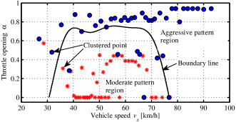
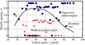
where and and, here, and are the arithmetic sequences with initial value , end value and interval value . For SVM training, the initial value () is set as (). After training the data set, we get the optimal value () is (), i.e., and . Based on above descriptions, the driving patterns are classified using MC-SVM method and the optimal separating hyperplane is produced, as shown in Fig. 2 and Fig. 3.
II-C -means Clustering
As one of the direct methods to analyses and extracts feature parameters from the large volume of raw data, the aim of clustering method is to provide objective and stable classifications [18]. Objective in the case means that the analysis of the same set of drivers using the same sequence of numerical methods results in the same classification. Stable denotes that the classification remains the same under a wide variety of additions of drivers.
Assume that a set of training examples () is recorded. is the set of all driving data sets and is the set of all labels that drivers subject to. Generally speaking, the driving data would be thousands of data points () and they are highly overlapped data sets. To reduce the number of support vectors and separate the raw feature parameters for different types driving patterns, the -MC method is applied. For any data point () , the remaining data sets would be clustered and generating a new cluster, if the remaining data could meet the following condition
| (6) |
where is a constant parameter that determine the center-radius of new clusters, and must have the same label. Therefore, the application of -MC could refine the raw data into a new set. -MC is used to partition the raw data sets into () clusters, forming a set . The is the subset of set . In this paper, the -MC is calculated by optimizing the following objective function:
| (7) |
where is the mean of point in set , , and is the number of observations. The adopted clustering algorithm can be found in [19].
II-D Training Results Analysis
Two typical drivers are discussed in the training results. For moderate driver in Fig. 2, he prefers lower speed ( km/h) with smaller throttle openings () when passing a curve road. When vehicle speed km/h, the moderate driver prefers a smaller throttle opening (). When the vehicle speed reaches to certain threshold ( km/h), the moderate drive prefers less opportunities in the speed range, km/h, than the aggressive driver. According to the Fig. 2, the moderate driver rarely drives the vehicle with speed of larger than km/h. For aggressive driver in Fig. 2, they prefer a larger throttle opening most of the case, though there are some times that the small throttle opening is selected. For the vehicle speed, the aggressive driver prefers has less opportunity to drive vehicle at speed of the range of km/h and have a higher opportunity to drive at speed range of km/h, in which the moderate driver scarcely does.
For moderate driver in Fig. 3, he prefers to drive vehicle with speed range of and a small throttle opening ranging from to . For the aggressive driver , he prefers a lager throttle opening than the moderate driver though the vehicle has a lower speed in km/h, which means that the aggressive driver prefers a lager acceleration. When km/h, the aggressive driver prefers to chose a lager throttle opening than the moderate driver. Specially, according to Fig. 3, we can conclude that the aggressive driver is incline to a higher speed ( km/h) than the moderate driver when they drive on the curve road.
III Experiments in Driving Simulator
In this section, the driver simulator and the collection of the training data are discussed.
III-A Driving Simulator
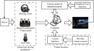
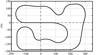
All the experimental data are collected in a driving simulator. The driving simulator consists of five main parts (Fig. 4). The game-type driving peripherals are used to collect the driver’s operating signals, i.e., steering wheel angle, brake pedal displacement, throttle opening. The virtual scenarios, including the vehicle, roads, and driving facilities, are designed through 3Ds Max software and Vizard software. The vehicle dynamics model is built using Matlab/Simulink, and a 2-DOF vehicle model is used. The driving environment is considered normal and the road friction is set as . Fig. 5 shows the road files we designed.
III-B Training-Data Collection and Experiments
The driving simulator could record a list of driving parameters such as vehicle speed, vehicle position, steering wheel angle, braking pedal displacement, throttle opening, at a sample frequency of 50 Hz. In the experiment, every driver should be familiarized with the test course and the driving simulator before running an experiment. Two typical types of the human driver, including four aggressive and four moderate, are involved. To rule out other factors such as the age and gender, all participants are male and aging between 22 27 years. Before running the tests, the driving pattern for each driver is determined by a questionnaire way. For each participant, the participant drives vehicle in the simulator more than ten times and every driver is manually labeled the driving pattern such as aggressive or moderate driver before running.
IV Recognition Performance Evaluation
The assessment method for the proposed recognizer, i.e., MC-SVM, is described in this section and the testing results are presented and discussed.
IV-A Evaluation Method
To evaluate recognition performance of the proposed recognition method, a well-known evaluation scheme, called cross-validation, is utilized. For all recorded data from the driving simulator, they are divided into subsets of equal size. Then, (, ) arbitrary subsets of all data sets are used to assessing the performance of classifier trained by the rest subsets. This method is called Leave--out Cross-validation (LO-CV). Here, the value of is set as . The accuracy of driving-pattern recognizer is defined as:
-
•
For the aggressive driver:
(8) -
•
For the moderate driver
(9)
where denotes the {} number of {} driving pattern. , and the symbol represents the correct choice. For example, represents the number of the clustering points that are correctly classified into the moderate pattern region for the moderate driver.
IV-B Testing Results and Analysis
For different testing data sets , the test results with corresponding to training data sets are conducted using off-line and on-line method. Then, the comparisons between MC-SVM and SVM are presented.
IV-B1 Off-line Testing
For off-line test, all the data are recorded and clustered first, and then the clustered testing data is used for evaluation. The off-line test results of testing data corresponding to the training data sets in Fig. 2 and Fig. 3 are shown in Fig. 6, Fig.7, and Table I. The symbol denotes the first group of drivers with driving pattern. From the Table I, it is obvious that the MC-SVM method has more benefits than the traditional SVM method on the recognition of driving styles. For the first group of drivers, the MC-SVM method is more efficient to recognizing the aggressive driver than SVM method, but not improvement on recognizing the moderate drivers. For the second group of drivers, the MC-SVM method has greatly benefits for recognizing both driving patterns, improve recognition accuracy by and .
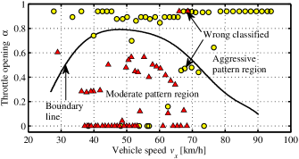
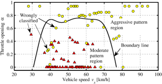
IV-B2 On-line Testing
We assume that the human driver’s driving pattern are treated as constant in a fixed time interval , is the current time and is the fixed time span. In this paper, the past information or driving pattern of the human driver during a fixed time span is adopted to represent the current driving pattern. Therefore, the current driving style is described as follows:
| (10) |
where is the clustering point based on the past time span and . Therefore, the data sequence of driving data can be clustered in the time span , generating clustering data sets. The testing results are shown in Fig. 8, Fig. 9, and Table I. According to the Table I, we can make conclusion that the MC-SVM method has a higher accuracy for recognition of driving patterns than SVM. For the first group of drivers, the accuracy of recognition is improved by and for the aggressive driver and moderate driver, respectively. For the second group, the accuracy of recognition is improved by and for the aggressive and moderate driver, respectively.
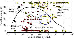
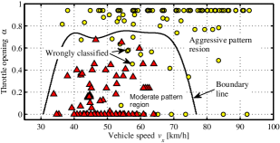
| Method | |||||
|---|---|---|---|---|---|
| MC-SVM | off-line | 77.78% | 92% | 79.49% | 95% |
| on-line | 87.04% | 94.92% | 82.72% | 100% | |
| SVM | off-line | 74.25% | 93.28% | 75.35% | 85.43% |
IV-C Time-Cost Analysis
In this section, to show the time-saving benefits of MC-SVM, one data set for testing is selected from the all of the datasets, and then the remaining data sets are used for training. The training time is listed in Table. II using MC-SVM and SVM, where , and , , [s] is the calculation time. For MC-SVM method, [s] consists of the clustering time and training time, and for SVM method, [s] is the training time. Because the testing time is very short, we neglected it here. According to Table II, we can know that the MC-SVM method can shorten time greatly, though the on-line recognition efficiency is down slightly, compared with the SVM method.
| MC-SVM | SVM | |||||
| [s] | [s] | |||||
| 169.35 | 78.89% | 82.07% | 740.18 | 85.46% | 88.19% | |
V Conclusion
A rapid pattern-recognition method, called MC-SVM, is developed by combining the -means clustering and SVM, and subsequently applied to recognize driver’s curve-negotiating patterns, i.e., aggressive and moderate. The kMC-SVM, compared with SVM, can not only shorten the recognition time but improve the recognition for classification issues that are not linearly separable. First, to reduce the number of support vectors, the -means clustering method is applied, clustering the original data sets into subsets. And then, based on the clustering results, the SVM is applied to generate the hyperplane for datasets with different labels. Last, the cross-validation experiments is designed to shown the benefits of the proposed method. The testing results show that the MC-SVM is able to not only shorten the training time for classification model, but improve recognition, compared with SVM method.
References
- [1] W. Wang, J. Xi, and J. Wang, “Human-centered feed-forward control of a vehicle steering system based on a driver’s steering model”, 2015 American Control Conference, Chicago, IL, pp. 3361 – 3366, July 2015.
- [2] M. Bichi, G. Ripaccioli, S. Di Cairano, D. Bernardini, A. Bemporad, and I.V. Kolmanovsky, “Stochastic model predictive control with driver behavior learning for improved powertrain control,” in 49th IEEE Conference on Decision and Control, Hilton Atlanta Hotel, Atlanta, GA, USA, pp. 6077 – 6082, Dec. 15 – 17, 2010.
- [3] M. Okamoto, S. Morimoto, M. Ohashi, and K. Uchida, “Automobile on-demand gear-shift control including driver characteristics,” in 2010 IEEE Multi-Conference on Systems and Control, Yokohama, Japan, pp. 896 – 901, Sep. 8 – 10, 2010.
- [4] J. Wang, L. Zhang, D. Zhang, and K. Li, “An adaptive longitudinal driving assistance system based on driver characteristics,” IEEE Transaction on Intelligent Transportation Systems, vol. 14, no. 1, pp. 1 – 12, Mar. 2013.
- [5] P. Angkititrakul, R. Terashima, and T. Wakita, “On the use of stochastic driver behavior model in lane departure warning,” IEEE Transaction on Intelligent Transportation Systems, vol. 12, no. 1, pp. 174 – 183, Mar. 2011.
- [6] M. Plöchl and J. Edelmann, “Driver models in automobile dynamics application,” Vehicle System Dynamics, vol. 45, nos. 7 – 8, pp. 699 – 741, July – August 2007.
- [7] W. Wang and J. Xi, “Study of semi-active suspension control strategy based on driving behavior characteristics”, International Journal of Vehicle Design, vol. 68, nos. 1 – 3, pp. 141 – 161, 2015.
- [8] C.C. Macadam, “Understanding and modelling the human driver,” Vehicle System Dynamics, vol. 40, nos. 1 – 3, pp. 101 –134, 2003.
- [9] W. Wang, J. Xi, and H. Chen, “Modeling and recognizing driver behavior based on driving data: a survey,” Mathematical Problems in Engineering, vol. 2014, Article ID 245641, 20 pages, 2014.
- [10] E. Tadesse, W. Sheng, and M. Liu, “Driver drowsiness detection through HMM based dynamic modeling,” in 2014 IEEE International Conference on Robotics & Automation, Hong Kong Convention and Exhibition Center, Hong Kong, China, pp. 4003 – 4008, May 31 - June 7, 2014.
- [11] V. Gadepally, A. Krishnamurthy, and Ü. Özgüner, “A framework for estimating driver decisions near intersections,” IEEE Transaction on Intelligent Transportation Systems, vol. 15, no. 2, pp. 637 – 646, Apr. 2014.
- [12] D. Mitrivić, “Reliable method for driving events recognition,” IEEE Transaction on Intelligent Transportation Systems, vol. 6, no. 2, pp. 198 – 205, Jun. 2005.
- [13] M. Sundbom, P. Falcone, and J. Sjöberg, “Online driver behavior classification using probabilistic ARX models,” in Proceedings of the 16th International IEEE Annual Conference on Intelligent Transportation Systems, pp. 1107 – 1112 , Hague, Netherlands, Oct. 2013.
- [14] T. Akita, S. Inagaki, T. Suzuki, S. Hayakawa, and N. Tsuchida, “Hybrid system modeling of human driver in the vehicle following task,” in SICE Annual Conference 2007, Kagawa University, Japan, , pp. 1122 – 1127, Sept. 2007.
- [15] S. Sekizawa, S. Inagaki, T. Suzuki, S. Hayakawa, N. Tsuchida, T. Tsuda, and H. Fujinami, “Modeling and Recognition of Driving Behavior Based on Stochastic Switched ARX Model,” IEEE Transaction on Intelligent Transportation Systems, vol. 8, no. 4, pp. 593 – 606, Dec. 2007.
- [16] Y. Zhang, W.C. Lin, and Y.S. Chin, “A pattern-recognition approach for driving skill characterization,” IEEE Transaction on Intelligent Transportation Systems, vol. 11, no. 4, pp. 905 – 916, Dec. 2010.
- [17] B. Higgs and M. Abbas, “Segmentation and clustering of car-following behavior: recognition of driving patterns,” IEEE Transactions on Intelligent Transportation Systems, vol. 16, no. 1, pp. 81 – 90, Feb. 2015.
- [18] B.S. Everitt, S. Landau, M. Leese, and D. Stahl, Cluster Analysis, 5th Edition, John Wiley & Sons Ltd., Publication, 2011.
- [19] D. Mackay, Information Theory, Inference, and Learning Algorithms, Cambridge University Press, 2003.
- [20] A.O. Hatch, S. Kajarekar, and A. Stolcke, “Within-class covariance normalization for SVM-based speaker recognition,” in 2006 and 9th International Conference on Spoken Language Processing, vol. 3, pp 1471 – 1474, 2006.
- [21] C. Cusano, G. Ciocca, and R. Schettini, “Image annotation using SVM,”, in Proc. SPIE 5304, Internet Imaging, vol. 330, Dec. 22, 2003.
- [22] C. Schuldt, I. Laptev, and B. Caputo, “Recognizing human actions: a local SVM approach,” in Proceedings of the 17th International Conference on Pattern Recognition, vol. 3, 2004
- [23] C.M. Bishop, Pattern Recognition and Machine Learning, Information Science and Statistics, Verlag New York Inc., 2006.
- [24] C.W. Hsu, C.C. Chang, and C.J. Lin, “A practical guide to support vector classification,” 2003.