Enhanced Playback of Automated Service Emulation Models Using Entropy Analysis

Abstract

Service virtualisation is a supporting tool for DevOps to generate interactive service models of dependency systems on which a system-under-test relies. These service models allow applications under development to be continuously tested against production-like conditions. Generating these virtual service models requires expert knowledge of the service protocol, which may not always be available. However, service models may be generated automatically from network traces. Previous work has used the Needleman-Wunsch algorithm to select a response from the service model to play back for a live request. We propose an extension of the Needleman-Wunsch algorithm, which uses entropy analysis to automatically detect the critical matching fields for selecting a response. Empirical tests against four enterprise protocols demonstrate that entropy weighted matching can improve response accuracy.

1 Introduction

Continuous delivery is an emerging practice in Software Engineering which aims to compress the release cycle such that a completed developer change can be quickly released (within a timeframe of hours) to the end-user. It aims to satisfy the business demand for agility and can be applied to both Cloud computing and on-premise software.

Continuous delivery relies on automating all stages of the release cycle, including software builds, unit testing, integration testing, performance testing and end-user environment testing. For continuous delivery, fully automated tests need to be performed in “production like conditions” [13]. For on-premise enterprise software, this is particularly challenging. Each enterprise environment is unique. Furthermore, a software system-under-test (SUT) will be integrated with other systems, such that its behaviour depends on the interactions it makes with the other systems. As a consequence, upgrading, replacing or installing a new service in an enterprise environment is high risk. To be confident the SUT can successfully operate in production, one needs an accurate replication of the real dependency services’ behaviours (including any bugs), at their current versions and configurations. The traditional approach includes having a test environment which is a close replication of the production environment. This is not only expensive to build and maintain, but is difficult to automate making, this approach incompatible with continuous delivery.

Service virtualisation [18] (also known as service emulation) is a technology to build accurate interactive models of the dependency services on which a system-under-test relies. This is achieved by recording on-the-network interactions between a system-under-test and other services in the production environment, and using this as the basis for building a virtualised service model. Since the models are built directly from the real dependency services, their interactive behaviour may be quite accurate. Furthermore, service models are conducive to automation, as they can be easily distributed and incorporated into automated tests. IT operations staff, quality assurance teams and application developers, may all make use of virtual service models to test software in production like conditions. Service virtualisation is, therefore, a critical tool for accelerating the software release cycle and supporting the ultimate goal of continuous delivery.

Service virtualisation requires a Data Protocol Handler (DPH) for every dependency service on which the system-under-test relies. The DPH processes the syntax and semantics of recorded network messages – headers are identified, operations and arguments are extracted, and business rules are identified. Service virtualisation tools provide a set of predefined DPHs covering the most commonly used protocols. However, some of the dependency services may use a less common, and therefore unsupported, protocol. Examples of this include proprietary systems, legacy systems, specialised domain applications, custom built or in-house applications, and mainframe systems. Yet for the system-under-test to be able to operate in a virtualised environment, it is essential that all of the dependency systems be virtualised. If even one of the dependency systems is missing, production like test can, in general, not be performed.

For any unsupported protocol, a custom DPH needs to be written. This may require extensive hours of programming as well as detailed knowledge of the target protocol, provided by thorough documentation and application specific knowledge given by the application architect. In practice such detailed knowledge is often unavailable or incomplete. For example, documentation may be missing, not updated, or the original application architect may have left the organisation. Without the required knowledge, writing the custom DPH becomes impossible, causing the entire service virtualisation project to fail.

To address this gap, an alternative method for service virtualisation was proposed [7], the method, dubbed opaque service virtualisation, uses the Needleman-Wunsch algorithm [19] to perform byte-level matching, when selecting a response from the opaque service model to replay. This method assumes no knowledge of the target protocol, enabling a service to be modelled automatically, even in the absence of the expert knowledge that would otherwise be required.

The previous opaque service virtualisation technique [7] has limited accuracy when a response of the wrong operation type is replayed. Since there is no knowledge of the protocol or message structure, there is no way to prioritise matching the operation type over other parts of the message (i.e. the payload). We propose an extension to opaque service virtualisation, whereby entropy analysis is used is used to prioritise matching responses for the correct operation type. The technique extends the Needleman-Wunsch algorithm to perform an entropy weighted match.

2 Related Work

The most common approach to recreating a production like environment for a system-under-test is to use virtual machines [15]. Implementations of the services are deployed on virtual machines and communicated with by the system under test. Major challenges with this approach include configuration complexity [10] and the need to maintain instances of each and every service type in multiple configurations [11]. Recently, cloud-based testing environments [1] as well as containerisation [6] have emerged to mitigate some of these issues.

Emulated testing environments for enterprise systems, relying on service models, is another approach. When sent messages by the system under test, the emulation responds with approximations of “real” service response messages [2]. Kaluta [12] is proposed to provision emulated testing environments. Challenges with these approaches include developing the models, lack of precision in the models, especially for complex protocols, and ensuring robustness of the models under diverse load conditions [23].

Recording and replaying message traces is an alternative approach. This involves recording request messages sent by the system under test to real services and response messages from these services, and then using these message traces to ‘mimic’ the real service response messages in the emulation environment [5]. Some approaches combine record-and-replay with reverse-engineered service models. CA Service Virtualization [18] is a commercial software tool, which can emulate the behaviour of services. The tool uses built-in knowledge of some protocol message structures to model services and mimic interactions automatically.

Roadmaps of research challenges relating to continuous delivery broadly have also been proposed [4, 9]. Entropy analysis has been used in other domains, for example in anti-malware research, entropy profiles have been used to classify packers [8].

3 Response Playback Framework

#	Request	Response
1	{id:001,op:S,sn:Du}	{id:001,op:SearchRsp,result:Ok,
		gn:Miao,sn:Du,mobile:5362634}
2	{id:013,op:S,sn:Versteeg}	{id:013,op:SearchRsp,result:Ok,
		gn:Steve,sn:Versteeg,mobile:9374723}
3	{id:024,op:A,sn:Schneider}	{id:024,op:AddRsp,result:Ok}
4	{id:275,op:S,sn:Han}	{id:275,op:SearchRsp,result:Ok,
		gn:Jun,sn:Han,mobile:33333333}
5	{id:490,op:S,sn:Grundy}	{id:490,op:SearchRsp,result:Ok,
		gn:John,sn:Grundy,mobile:44444444}
6	{id:773,op:S,sn:Hine}	{id:273,op:SearchRsp,result:Ok,
		sn:Hine,mobile:123456}
7	{id:887,op:A,sn:Will}	{id:887,op:AddRsp,result:Ok}
8	{id:906,op:A,sn:Hine}	{id:906,op:AddRsp,result:Ok}

Table 1: Directory Service Interaction Library Example

Opaque service virtualisation consists of two parts:

1. Record an interaction library – a sample set of messages exchanges between a system-under-test and a dependency service (the target service). These messages may be collected using a network analyser tool, such as WireShark, or logged through a proxy.

2. Deploy an emulation of the target service. The emulator receives live requests on the network from the system-under-test. The emulator searches the interaction library for the nearest matching request, and plays back the corresponding response.

We will now give a playback example and then describe in detail the previous approach to the response selection step.

3.1 Non-Weighted Playback Example

Table 1 shows a small example interaction library. It is from a fictional directory service protocol that has some similarities to the widely used LDAP protocol [20], but is simplified to make our running example easier to follow. Our example protocol uses a JSON encoding. The transaction library contains two kinds of operations: add and search. Add requests contain the field op:A, whereas search requests have op:S. The add and search response operations are specified with the fields op:AddRsp and op:SearchRsp, respectively.

Suppose we receive a live search request, for example, {id:552,op:S,sn:Hossain}. Using the Needleman-Wunsch response selection method [7], then request 4 ({id:275,op:S, sn:Han}, $dist$=0.125) is the nearest request in the interaction library and the emulator will replay a search response. For this case the behaviour is correct.

Now suppose we receive another live search request:
{id:024,op:S,sn:Schneider}. When selecting a response, request 3 ({id:024,op:A,sn:Schneider}, $dist$=0.019) is a nearer match than request 4 ({id:275,op:S,sn:Han}, $dist$= 0.15), even though the latter is a search request and the former is an add request. Due to there being no prioritisation for matching the operation type characters (op:A) over the payload characters, a response of the wrong operation type may be played back.

3.2 Definitions

We define a number of constructs needed to express our framework more formally. We start with the notion of the most basic building block, the set of message characters, denoted by $\mathcal{C}$. We require equality and inequality to be defined for the elements of $\mathcal{C}$. For the purpose of our study, $\mathcal{C}$ could comprise of a set of valid bytes that can be transmitted over a network or characters from a character set (such as ASCII or Unicode) or the set of printable Characters as a dedicated subset. Furthermore, we define $\mathcal{M}$ to be the set of all (possibly empty) messages that can be defined using the message characters. A message $m\in\mbox{$\mathcal{M}$}$ is a non-empty, finite sequence of message characters $c_{1}c_{2}c_{3}\ldots c_{n}$ with $c_{i}\in\mbox{$\mathcal{C}$},1\leq i\leq n$.

Without loss of generality, we assume that each request is always followed by a single response. If a request does not generate a response, we insert a dedicated “no-response” message into the recorded interaction traces. If, on the other hand, a request leads to multiple responses, these are concatenated into a single response.

A single interaction $I$ consists of a request, denoted by Rq, as well as the corresponding response, denoted by Rp. Both Rq and Rp are elements of $\mathcal{M}$ and we write $(\mbox{\it Rq},\mbox{\it Rp})$ to denote the corresponding request/response pair.

An interaction trace is defined as a finite, non-empty sequence of interactions, that is, $I_{1}I_{2}I_{3}\ldots I_{n}$. Finally, we define the set of interactions $\mathcal{I}$ as a non-empty set of interaction traces.

3.3 Non-Weighted Response Selection

Our previous framework consisted two main processing steps: (i) given an incoming request from the system-under-test to a virtual service model, we search for a suitably “similar” request in the previously recorded interaction traces. (ii) Our system then synthesizes a response for the incoming request based on the similarities in the request itself and the “similar” request identified in the interaction traces, as well as the recorded response of the “similar” request.

Using the definitions introduced above, our framework can thus be formalized as below. To facilitate the presentation, we denote ${\mbox{\it Rq}}_{in}$ as the incoming request and the interaction library $I^{*}({\mbox{$\mathcal{I}$}})$ as the set of all interactions in $\mathcal{I}$.

${\mbox{\it Rp}}_{out}=\mathbf{\mbox{$trans$}}\ ({\mbox{\it Rq}}_{in},{\mbox{\it Rq}}_{sim},{\mbox{\it Rp}}_{sim})$

with

• ${\mbox{$({\mbox{\it Rq}}_{sim},{\mbox{\it Rp}}_{sim})$}}\in I^{*}({\mbox{$\mathcal{I}$}})$; and
  

• $\forall\;{\mbox{$({\mbox{\it Rq}}_{i},{\mbox{\it Rp}}_{i})$}}:{\mbox{$dist$}}({\mbox{\it Rq}}_{in},{\mbox{\it Rq}}_{sim})\leq{\mbox{$dist$}}({\mbox{\it Rq}}_{in},{\mbox{\it Rq}}_{i})$

where $dist$ and $trans$ denote user-defined distance and translation functions, respectively, allowing the framework to be tailored for the specific needs of given context.

The distance function $dist$ is used to compute the distance between two requests. We require (i) the distance of a message $m$ with itself to be zero, that is ${\mbox{$dist$}}(m,m)=0$, and (ii) the distance between two non-identical messages $m_{1}$ and $m_{2}$ to be greater than zero. Depending on what kind of distance function is used, a different pre-recorded request will be chosen to be the most “similar” to the incoming request. We used the Needleman-Wunsch edit distance [19] as the basis for $dist$.

The translation function’s responsibility is to synthesize a response for the incoming request. As a simplification of our work, we made the decision to ignore temporal properties in our framework, that is, the synthesized response solely depends on the incoming request and the recorded interaction traces, but not on any previously received or transmitted requests or responses, respectively. Adding a temporal dimension to the framework is part of our future work.

3.4 Needleman-Wunsch

The Needleman-Wunsch algorithm [19] is a dynamic programming algorithm for computing the edit distance between two sequences. Needleman-Wunsch finds the globally optimal alignment for two sequences of symbols in $O(n_{1}\!\cdot\!n_{2})$ time, where $n_{1}$ and $n_{2}$ are the lengths of the sequences.

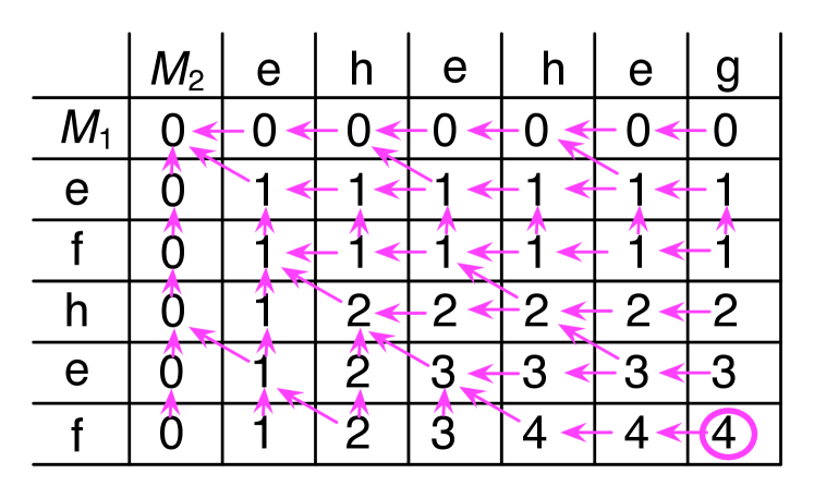
(a) $F$-matrix fill

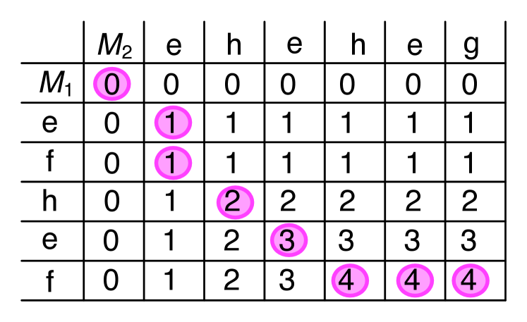
(b) $F$-matrix trace back

Figure 1: Needleman-Wunsch example of aligning $M_{1}=\text{`efheh'}$ and $M_{2}=\text{`eheheg'}$, using $d_{\rm identical}=1,d_{\rm differing}=-1,d_{\rm gap}=0$.

Needleman-Wunsch progressively constructs a matrix $F$, using a scoring function $S(a,b)$ to score pairs of aligned symbols:

$$S(a,b)=\begin{cases}d_{\rm identical}&~{}\text{if}~{}a=b\\ d_{\rm differing}&~{}\text{otherwise}\\ \end{cases}$$ (1)

where $d_{\rm identical},d_{\rm differing}$ are constants. The constant $d_{\rm gap}$ is the gap penalty constant.

Needleman-Wunsch has three stages. To align two sequences $M_{1}$ (of length $n_{1}$) and $M_{2}$ (length $n_{2}$):

1. An $(n_{1}+1)\times(n_{2}+1)$ matrix $F$ is constructed, with rows and columns labelled from 0..$n_{1}$ and 0..$n_{2}$, respectively. Row 0 and column 0 are initialised to 0.

2. $F$ is calculated progressively. At each cell:

   $$F_{i,j}={\it max}\left\{\begin{array}[]{l}F_{i-1,j-1}+S(M_{1}(i),M_{2}(j))\\ F_{i,j-1}+d_{\rm gap}\\ F_{i-1,j}+d_{\rm gap}\\ \end{array}\right.$$ (2)

   (See Figure 1 for example.)

3. $F_{n_{1},n_{2}}$ gives $\mbox{$score$}(M_{1},M_{2})$, the optimal alignment score of $M_{1}$ and $M_{2}$. The trace back step (see Figure 1) captures the alignment.

For example (in Figure 1), the strings $M_{1}=\text{`efheh'}$ and $M_{2}=\text{`eheheg'}$ have an alignment score $\mbox{$score$}=4$ and are aligned as:

efheh${\boldsymbol{\star}}$${\boldsymbol{\star}}$

e${\boldsymbol{\star}}$heheg

To normalise for sequence length, we define the distance of $M_{2}$ relative to $M_{1}$ as:

$$\mbox{$dist$}(M_{1},M_{2})=\frac{\mbox{$score$}(M_{1},M_{2})-\mbox{$score$}_{\rm min}}{\mbox{$score$}_{\rm max}-\mbox{$score$}_{\rm min}}$$ (3)

where $\mbox{$score$}_{\mathrm{max}}$ denotes the maximum possible alignment score and $\mbox{$score$}_{\mathrm{min}}$ the minimum possible alignment score for $M_{1}$ as defined by equations 4 and 5, respectively.

$${\mbox{$score$}_{\mathrm{max}}(M_{1})}=\sum_{i=1}^{|M_{1}|}S(M_{1}(i),M_{1}(i))$$ (4)

$${\mbox{$score$}_{\mathrm{min}}(M_{1})}=\sum_{i=1}^{|M_{1}|}S(M_{1}(i),\varnothing)$$ (5)

where $\varnothing\not\in\mbox{$\mathcal{C}$}$ is a special symbol not in the character set.

4 Entropy Weighted Approach

We now propose a method of predicting which parts of a message contain the operation type and other structural information, using entropy analysis. Our method assumes no prior knowledge of the protocol message structure. We make use of the observation that the parts of the message which contain operation type and structural information are more stable (have less possibilities) than the parts of the message containing payload information. We perform an entropy analysis on the interaction library to derive a weightings vector, which is applied to prioritise matching for the Needleman-Wunsch distance calculation. The character positions with a low entropy (stable) are given a high weighting, and character positions with high entropy (unstable) are given a low weighting. Figure 2 depicts an overview of our approach.

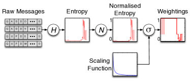
Figure 2: Transformation steps in deriving a set of entropy weights

Let $R=(r_{i,j})$ be a matrix of requests of normalised length:

$$r_{i,j}=\begin{cases}\mbox{\it Rq}_{i,j}&\text{if}\ j<|\mbox{\it Rq}_{i}|\\ \lambda&\text{otherwise}\end{cases}$$ (6)

where $\mbox{\it Rq}_{i,j}$ is the $j$th character of the $i$th request in the interaction library $I^{*}({\mbox{$\mathcal{I}$}})$, $1\leq i\leq|\mbox{$I^{*}({\mbox{$\mathcal{I}$}})$}|,1\leq j\leq L$. $L={\it max}\{|\mbox{\it Rq}_{i}|\}$ is the length of the longest request, and $\lambda\not\in\mbox{$\mathcal{C}$}$ is a special character to denote a missing value.

Let $q_{j}(c)$ be the relative frequency of the character $c\in\mbox{$\mathcal{C}$}$ for the $j$th column of $R$. Let the set $Q_{j}=\{q_{j}(c):c\in\mbox{$\mathcal{C}$}\}$ be the set of relative frequencies for all characters at the $j$th column position of $R$.

To calculate a weightings vector, we require three functions:

• Let $H:{\mbox{$\mathbb{R}$}}^{n}\rightarrow{\mbox{$\mathbb{R}$}}$ be a method for calculating the entropy of the set of real numbers.

• Let $N:{\mbox{$\mathbb{R}$}}\rightarrow[0,1]$ be a normalisation function.

• Let $\sigma:[0,1]\rightarrow[0,1]$ be a scaling function.

We define the weightings vector ${\bf w}=(w_{1},w_{2},...w_{L})$, which gives a weighting for each column in the matrix $R$, with:

$$w_{j}=\sigma(N(H(Q_{j})))$$ (7)

4.1 Entropy Measures

We calculated the entropy of each column position of the matrix $R$, considering three alternative entropy methods:

• Shannon Index [21] is based on the weighted geometric mean of the relative frequencies of the characters, as given by Equation 8.

  $$H_{\rm Shannon}(Q)=-\sum^{|Q|}_{q_{k}\in Q}q_{k}\log q_{k}$$ (8)

• Richness [14] is a simple count of how many different characters occur at a give column, i.e.

  $$H_{\rm Richness}(Q)=|Q^{\prime}|,\text{~{}where~{}}Q^{\prime}=\{q_{k}:q_{k}\in Q\land q_{k}>0\}$$ (9)

• The Simpson Index [22] is another measure of the concentration of types. It is defined as:

  $$H_{\rm Simpson}(Q)=\sum^{|Q|}_{q_{k}\in Q}q_{k}^{2}$$ (10)

4.2 Range Normalisation

The entropy measures described in Section 4.1 have differing ranges. We introduce a normalisation step, such that the entropy measured in each column of R is in the range [0,1]. Our normalisation function is:

$$N(x)=\frac{x-E_{\rm min}}{E_{\rm max}-E_{\rm min}}$$ (11)

where $E_{\rm min}={\it min}({\bf E}),E_{\rm max}={\it max}({\bf E}),{\bf E}=H({\bf Q})$.

4.3 Scaling Functions

The scaling function $\sigma$ serves two purposes: (i) to invert the normalised entropy value, such that low entropy positions are given a high value in the weighting vector, and (ii) to scale the differential between a high weighting and a low weighting.

We considered four types of scaling functions:

• A hyperbolic scaler of the form:

  $$\mbox{$\sigma$}_{\rm hyper}(x)=\frac{1}{(1+ax)^{c}}$$ (12)

  where $a>0$ and $c>0$ are scaling constants.

• An exponential scaler of the form:

  $$\mbox{$\sigma$}_{\rm exp}(x)=e^{-kx}$$ (13)

  where $k>0$ is a scaling constant.

• A sigmoid scaler of the form:

  $$\mbox{$\sigma$}_{\rm sigmoid}(x)=\frac{1}{1+e^{k(x-\tau)}}$$ (14)

  where $k>0$ is a scaling constant $0\leq\tau\leq 1$ is the threshold constant.

• A thresholding step function:

  $$\mbox{$\sigma$}_{\rm thresh}(x)=\begin{cases}1&\text{if}\ x\leq\tau\\ 0&\text{otherwise}\end{cases}$$ (15)

  where $0\leq\tau\leq 1$ is the thresholding constant.

4.4 Entropy Weighted Needleman-Wunsch

We propose a modified Needleman-Wunsch scoring matrix $F^{*}$ (replacing $F$). The initialisation and traceback steps for $F^{*}$ follow the same method as for standard Needleman-Wunsch (see cf.  3.4.) However for the progressive scoring calculation, weights are applied from the vector ${\bf w}$:

$$F^{*}_{i,j}={\it max}\left\{\begin{array}[]{l}F^{*}_{i-1,j-1}+w_{k}\!\cdot\!S(M_{1}(i),M_{2}(j))\\ F^{*}_{i,j-1}+w_{k}\!\cdot\!d_{\rm gap}\\ F^{*}_{i-1,j}+w_{k}\!\cdot\!d_{\rm gap}\\ \end{array}\right.$$ (16)

where $k={\it max}\{i,j\}$.

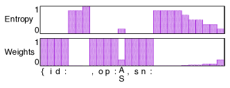
Figure 3: Example entropy and weights calculated from the interaction library in Table 1, using the Richness and hyperbolic scaler ($a=1,c=10$)

Figure 3 shows an example entropy and weights vectors calculated from the interaction library in Table 1 (using the Richness entropy method, and the hyperbolic scaler with $a=1,c=10$). Returning to our example from Section 3.1, by applying the entropy weighting method, a different response is selected. Using the weights vector from Figure 3, request 4 ($dist$=0.0066) now has a closer distance to the live request than request 3 ($dist$=0.019), thereby selecting a response of the correct operation type.

5 Experimental Evaluation

We wanted to evaluate the entropy-weighted response selection to answer the following research questions:

1. RQ1 (Comparison of Entropy Methods): what impact do the differing entropy methods have on the response accuracy?

2. RQ2 (Comparison of Scaling Functions): what is the impact of the scaling function on the response accuracy and the sensitivity of their parameters?

3. RQ3 (Relative Accuracy): what is the overall accuracy of the entropy weighted response selection relative to other methods?

5.1 Case Study Protocols and Traces

Protocol	Binary/Text	Fields	#Ops.	#Transactions
IMS	binary	fixed length	5	800
LDAP	binary	length-encoded	10	2177
SOAP	text	delimited	6	1000
Twitter (REST)	text	delimited	6	1825

Table 2: Message trace datasets.

In order to answer these questions, we applied our technique on message trace datasets from four case study protocols: IMS [16] (a binary mainframe protocol), LDAP [20] (a binary directory service protocol), SOAP [3] (a textual protocol, with an Enterprise Resource Planning (ERP) system messaging system services), and RESTful Twitter [24] (a JSON protocol for the Twitter social media service). We chose these four protocols because: (i) they are widely used in enterprise environments, (ii) they represent a good mix of text-based protocols (SOAP and RESTful Twitter) and binary protocols (IMS and LDAP), (iii) they use either fixed length, length encoding or delimiters to structure protocol messages, and (iv) each of them includes a diverse number of operation types, as indicated by the Ops column. The number of request-response interactions for each test case is shown as column #Transactions in Table 2.

Our message trace datasets are available for download at http://quoll.ict.swin.edu.au/doc/message_traces.html

Incoming Request	{id:15,op:S,sn:Du}
Expected Response	{id:15,op:SearchRsp,result:Ok,gn:Miao,sn:Du}
Valid Responses	{id:15,op:SearchRsp,result:Ok,gn:Miao,sn:Du}
	{id:15,op:SearchRsp,result:Ok,gn:Menka,sn:Du}
Invalid Responses	{id:15,op:AddRsp,result:Ok}
	{id:15,op:SearchRsp,result:Ok,gn:Miao},sn:Du

Table 3: Examples of valid and invalid emulated responses.

5.2 Compared Techniques

We compared the proposed entropy-weighted response selection with two other methods. The baseline for comparison was a hash lookup. If the hash code of an incoming request matched the hash code of a request in the transaction library, then the associated response was replayed (without any transformation). This approach can only work when a request is identical to the live request occurred in the recording. It is a standard record-and-replay approach used for situations where nothing is known about the protocol. Our second compared technique is the non-weighted Needleman-Wunsch response selection [7].

5.3 Accuracy Measurement

Cross-validation is a popular model validation method for assessing how accurately a predictive model will perform in practice. For the purpose of our evaluation, we applied the commonly used 10-fold cross-validation approach [17] to all four case study datasets.

We randomly partitioned each of the original interaction datasets into 10 groups. Of these 10 groups, one group is considered to be the evaluation group for testing our approach, and the remaining 9 groups constitute the training set. This process is then repeated 10 times (the same as the number of groups), so that each of the 10 groups will be used as the evaluation group once. When running each experiment with each trace dataset, we applied our approach to each request message in the evaluation group, referred to as the incoming request, to generate an emulated response. The entire cross validation process was repeated ten times for each experiment using different random seeds.

Having generated a response for each incoming request, we then used a validation script to assess the accuracy. The script used a protocol decoder to parse the emulated response and compared it to the original recorded response (the expected response) from the evaluation group. The emulated response was classified as valid or invalid, according to the following definitions:

1. Valid: the emulated response conformed to the message format of the protocol (i.e. was successfully parsed by the decoder) and the operation type of the emulated response was the same as the expected response. Note that contents of the emulated response payload may differ to the expected response and still be considered valid.

2. Invalid: the emulated response was not structured according to the expected message format of the protocol, or the operation type of the emulated response was different to the expected response.

5.4 Entropy Method Results (RQ1)

The three alternative entropy measure functions were used against the four datasets. Keeping the scaling method consistent (Hyperbolic scaler, $a=50,c=1$), the accuracy of the different methods is shown in Table 4. The Richness method was the best for the IMS dataset, and the Shannon Index was the best for LDAP. All of the entropy methods outperformed the non-weighted approach.

Entropy	IMS	LDAP	SOAP	Twitter
Method
None	77.4%	94.2%	100%	99.5%
Shannon	81.3%	94.9%	100%	99.5%
Richness	100%	91.6%	100%	99.5%
Simpson	89.9%	94.3%	100%	99.5%

Table 4: The response accuracy for the alternative entropy measures against the four datasets tested.

5.5 Scaling Function Results (RQ2)

The scaling functions were applied with varying parameters, keeping the entropy method consistent (Shannon Index). The results are shown in Figure 4. For the Hyperbolic scaler, the most significant results can be observed for IMS, where the accuracy increases from 80% to 99% as the $c$ scaling exponent is increased. Similarly for the Exponential scaler, accuracy for IMS increases with a higher exponent value. For the other datasets no dramatic differences are observed. The Thresholder scaler is very sensitive to the setting of the threshold $\tau$, and the optimal setting is different for each data set. The performance of the Sigmoid scaler appears fairly insensitive to the parameter settings.

(a) Hypberbolic scaler: $a$ sensitivity

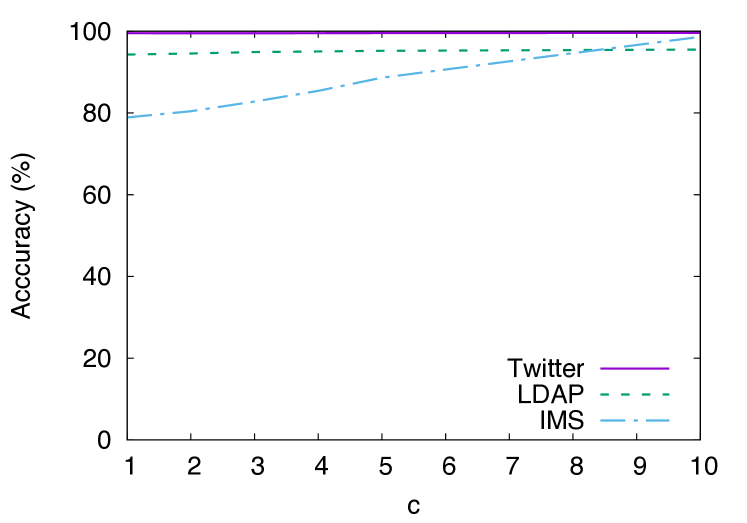
(b) Hyperbolic scaler: $c$ sensitivity

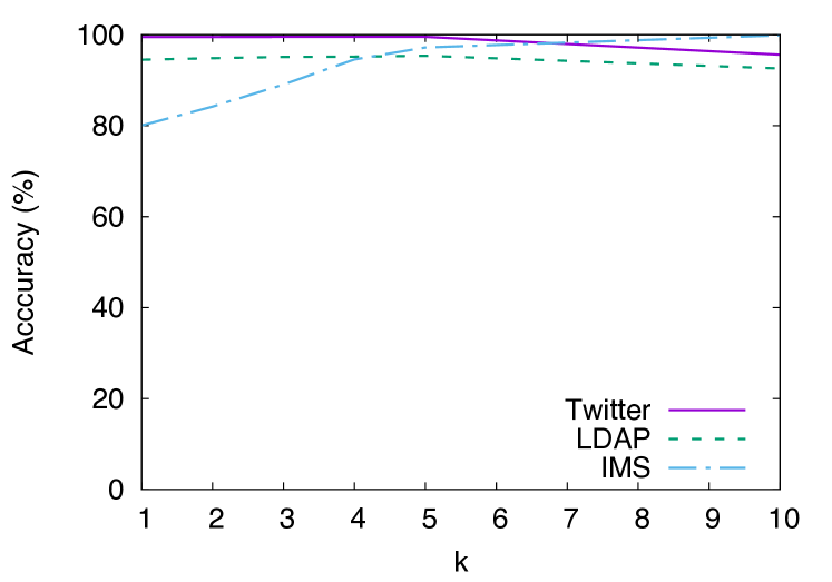
(c) Exponential scaler: $k$ sensitivity

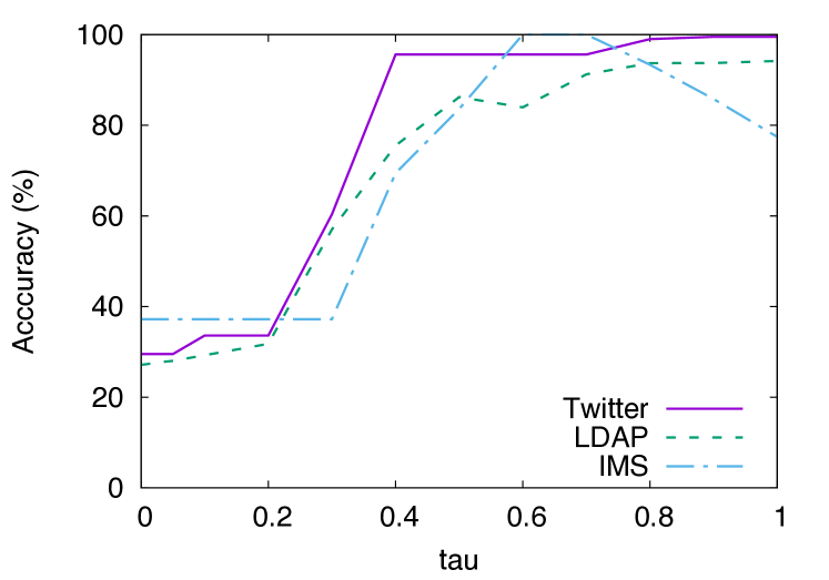
(d) Thresholding scaler: $\tau$ sensitivity

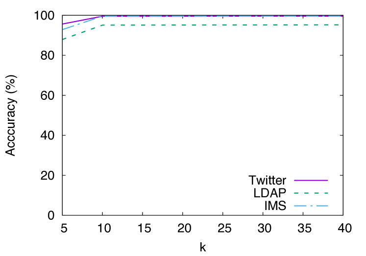
(e) Sigmoid scaler: $k$ sensitivity

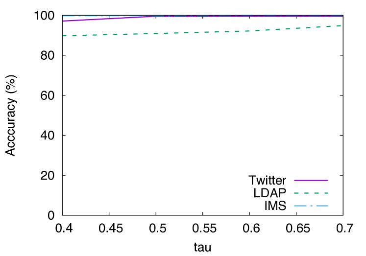
(f) Sigmoid scaler: $\tau$ sensitivity

Figure 4: Effect of scaling function parameters on response accuracy

5.6 Comparison to Baselines (RQ3)

Our results showed that the Shannon Index combined with the Hypberbolic scaler ($a=1,c=10$) gave high response accuracy for all datasets. Table 5 compares this method to the other response selection approaches. The entropy weighted method equalled or outperformed the other methods for all datasets. The most significant improvement occurs with IMS. There is a marginal improvement for LDAP and Twitter. SOAP already had 100% accuracy using the non-weighted method, but importantly the entropy weighting did not worsen this result.

Matching Method	IMS	LDAP	SOAP	Twitter
Hash Lookup	50%	5.36%	0.5%	30.1%
Non-Weighted NW	77.4%	94.2%	100%	99.5%
Entropy-Weight NW	98.6%	95.5%	100%	99.6%

Table 5: The response accuracy of entropy weighted matching versus other response selection methods

6 Discussion and Future Work

In the experiments, the entropy weighted method had a significant impact on improving the response accuracy for the IMS dataset, but had limited impact for the other three datasets. A key characteristic of IMS is that it uses fixed length encoding to delimit fields. This ensures the operation type will always be at the same character position. For the other datasets, the operation type can be at different positions in the message. We hypothesise that this is the cause of the decreased effectiveness for non-fixed width protocols. Further testing is required to confirm this.

Regarding the entropy measures tested, no one method was conclusively better. However we caution that Richness will be more sensitive to noisy data (with single data points distorting the results) whereas the Shannon and Simpson indices are more robust.

Future work will consider aligning all the messages in the interaction library before performing entropy analysis (using multiple sequence alignment). We expect this to improve results for variable width protocols, by increasing the probability that the operation type characters are aligned. Another extension is to cluster the interaction library first, and then perform a separate entropy analysis on each cluster.

7 Conclusion

Service virtualisation is an important tool for realising continuous delivery, by creating realistic service models of a system-under-test’s dependency services, thereby facilitating automated testing of production-like conditions. Opaque service virtualisation is a method for automatically deriving service models, even in the absence of a protocol decoder and other knowledge. We perform an entropy analysis on a recorded sample of the target service’s messages and then use an entropy weighted Needleman-Wunsch based similarity measure to select the best matching responses to play back to live requests. We have shown our entropy weighted approach can be used to improve the accuracy of opaque service virtualisation, particularly for fixed width protocols.

8 Acknowledgments

This research was supported by ARC grant LP150100892.

References

- [1] T. Banzai, H. Koizumi, R. Kanbayashi, T. Imada, T. Hanawa, and M. Sato. D-cloud: Design of a software testing environment for reliable distributed systems using cloud computing technology. In 10th IEEE/ACM International Conference on Cluster, Cloud and Grid Computing (CCGrid 2010), pages 631–636, Melbourne, Australia, 2010.
- [2] A. Bertolino, G. De Angelis, L. Frantzen, and A. Polini. Model-based generation of testbeds for web services. In Testing of Software and Communicating Systems, volume 5047, pages 266–282. 2008.
- [3] D. Box, D. Ehnebuske, G. Kakivaya, A. Layman, N. Mendelsohn, H. F. Nielsen, S. Thatte, and D. Winer. Simple Object Access Protocol (SOAP) 1.1, 5 2000. W3C Note 08 May 2000.
- [4] L. Chen. Continuous delivery: Huge benefits, but challenges too. IEEE Software, 32(2):50–54, 2015.
- [5] W. Cui, V. Paxson, N. C. Weaver, and R. H. Katz. Protocol-independent adaptive replay of application dialog. In Proceedings of the 13th Annual Network and Distributed System Security Symposium (NDSS 2006), pages 1–15, San Diego, California, USA, 2006.
- [6] Docker Inc. Docker. http://docker.com, 2015.
- [7] M. Du, J.-G. Schneider, C. Hine, J. Grundy, and S. Versteeg. Generating service models by trace subsequence substitution. In Proceedings of the 9th International ACM Sigsoft Conference on Quality of Software Architectures (QoSA 2013), pages 123–132, Vancouver, British Columbia, Canada, 2013.
- [8] T. Ebringer, L. Sun, and S. Boztas. A fast randomness test that preserves local detail. Virus Bulletin, 2008.
- [9] B. Fitzgerald and K.-J. Stol. Continuous software engineering and beyond: trends and challenges. In 1st International Workshop on Rapid Continuous Software Engineering, pages 1–9. ACM, 2014.
- [10] P. Godefroid. Micro execution. In 36th International Conference on Software Engineering (ICSE 2014), pages 539–549, Hyderabad, India, 2014.
- [11] J. Grundy, Y. Cai, and A. Liu. Softarch/mte: Generating distributed system test-beds from high-level software architecture descriptions. Automated Software Engineering, 12(1):5–39, Jan. 2005.
- [12] C. Hine. Emulating Enterprise Software Environments. Phd thesis, Swinburne University of Technology, Faculty of Information and Communication Technologies, 2012.
- [13] J. Humble. Continuous delivery vs continuous deployment. http://continuousdelivery.com/2010/08/continuous-delivery-vs-continuous-deployment/, 13 August 2010. (Accessed 19 January 2016).
- [14] L. Jost. The relation between evenness and diversity. Diversity, 2(2):207–232, 2010.
- [15] P. Li. Selecting and Using Virtualization Solutions: our Experiences with VMware and VirtualBox. Journal of Computing Sciences in Colleges, 25(3):11–17, 2010.
- [16] R. Long, M. Harrington, R. Hain, and G. Nicholls. IMS Primer. IBM International Technical Support Organisation, 2000.
- [17] G. J. McLachlan, K.-A. Do, and C. Ambroise. Analyzing Microarray Gene Expression Data. Wiley-Interscience, 2004.
- [18] J. Michelsen and J. English. Service Virtualization: Reality is Overrated. Apress, September 2012.
- [19] S. B. Needleman and C. D. Wunsch. A general method applicable to the search for similarities in the amino acid sequence of two proteins. Journal of Molecular Biology, 48(3):443–453, 1970.
- [20] J. Sermersheim. Lightweight Directory Access Protocol (LDAP): The Protocol, 6 2006. RFC 4511.
- [21] C. E. Shannon. A mathematical theory of communication. The Bell System Technical Journal, 27:379–423,623–656, 1948.
- [22] E. H. Simpson. Measurement of diversity. Nature, 1949.
- [23] J. Sun and T. Mannisto. Usefulness evaluation of simulation in server system testing. In 36th IEEE Computer Software and Applications Conference (COMPSAC 2012), pages 158–163, Turkey, 2012.
- [24] Twitter. The Twitter REST API, 2014.