Red, Straight, no bends: primordial power spectrum reconstruction from CMB and large-scale structure

Abstract

We present a minimally parametric, model independent reconstruction of the shape of the primordial power spectrum. Our smoothing spline technique is well-suited to search for smooth features such as deviations from scale invariance, and deviations from a power law such as running of the spectral index or small-scale power suppression. We use a comprehensive set of the state-of the art cosmological data: Planck observations of the temperature and polarisation anisotropies of the cosmic microwave background, WiggleZ and Sloan Digital Sky Survey Data Release 7 galaxy power spectra and the Canada-France-Hawaii Lensing Survey correlation function. This reconstruction strongly supports the evidence for a power law primordial power spectrum with a red tilt and disfavours deviations from a power law power spectrum including small-scale power suppression such as that induced by significantly massive neutrinos. This offers a powerful confirmation of the inflationary paradigm, justifying the adoption of the inflationary prior in cosmological analyses.

1 Introduction

All recent cosmological observations are in excellent agreement with the standard $\Lambda$CDM model: a spatially flat cosmological model, with matter-energy density dominated by a cosmological constant and cold dark matter, where cosmological neutrinos are effectively massless and where the primordial power spectrum of adiabatic perturbations is a (almost scale invariant) power law. State-of-the art cosmological observations such as those of the Planck satellite [1], measuring cosmic microwave background (CMB) anisotropies, provided us with very precise measurements of the parameters of the standard cosmological model [2].

Most cosmological analyses assume a power-law primordial power spectrum with a fixed spectral index, and deviations from this assumption are often in the form of a “running” of the spectral index.

A nearly scale invariant power spectrum is a generic prediction of the simplest models of inflation, but there are models with (small) deviations from this prediction (e.g., [3, 4, 5, 6]). Small deviations from scale invariance constitute a critical and generic prediction of inflation. For this reason a model-independent reconstruction of the primordial power spectrum (PPS) shape can be a powerful test of inflationary models.

Here we perform a minimally parametric reconstruction of the PPS using smoothing spline interpolation in combination with cross validation. This approach follows [7, 8, 9].

The idea is simple: we choose a functional form that allows a great deal of freedom in the shape of the deviations from a power-law. Because most models predict the PPS to be smooth, among the possible choices we use a smoothing spline. The ensuing challenge is to avoid over-fitting the data; a complex function that fits the data set extremely well is of no interest if we are simply fitting statistical noise. To prevent over-fitting we use cross-validation and a roughness penalty. The roughness penalty is an additional parameter that penalises a high degree of structure in the functional form. By performing cross-validation as a function of this penalty, we can judge the amount of freedom in the smoothing spline that the data require, without fitting the noise.

The Planck collaboration has performed an analysis with the same goals in mind, but with different methods [10]. They carried out both a parametric search for deviations from a power law, using a set of theoretically motivated shapes for the PPS, and a minimally parametric analysis to reconstruct the PPS. In all cases there is no strong evidence for deviations from a power law.

Our analysis differs from that of the Planck collaboration and from others existing in the literature as we analyse jointly a comprehensive set of state-of-the-art experiments probing the matter power spectrum and the latest Planck measurements.

Because we assume standard late-time evolution of density perturbations and consider both early-time observables (CMB) and late-time ones (i.e., large-scale structure), our reconstruction is also sensitive to late-time effects on structure formation. In particular a non-negligible neutrino mass would suppress the growth of structures below the neutrino free-streaming scale, inducing an “effective” loss of small scale power in our reconstructed PPS. Reconstructing in a model-independent way a possible neutrino signature on the shape of the matter power spectrum is of particular importance as [11, 12, 13, 14, 15, 16] claims that relatively large neutrino masses ($\Sigma_{\nu}\gtrsim 0.4$ eV) could solve the tension between CMB and local measurements, whilst other studies [17, 18, 19, 20, 21, 22, 23, 24] rule out this possibility.

The rest of the paper is organised as follows: in section 2 we briefly summarise the methodology adopted, the data chosen and how they are analysed. In section 3 we present our findings; we discuss and present the conclusions in section 4.

2 Methodology and datasets

2.1 Spline reconstruction

We perform a minimally-parametric reconstruction of the primordial power spectrum based on the method presented in [7] and further refined in [8, 9]. Here we only briefly summarise the approach; it is based on the cubic smoothing spline technique (for details see [25]). In this approach to recover a smooth function $f(x)$, given its value $f_{i}$ only on a set of $n$ points $x_{i}$, hereafter knots, one fits the pairs $(x_{i},f_{i})$ with a cubic spline $s(x)$. The spline, its first, and second derivatives are continuous on the knots by definition. The full function is then uniquely defined by the values at the knots and two boundary conditions. We choose to require that the jump in the third derivative across the first and last knots is forced to zero.

In our application the resulting spline function is the reconstructed primordial power spectrum. The $f_{i}$ are free parameters we wish to determine and we place the knots equally spaced in $\log k$ as it is the most conservative choice to recover deviations from a power law. The whole $s(k)$ is used as the PPS to compute the observables and evaluate the likelihood of the parameters $f_{i}$. Including the roughness penalty, the effective likelihood becomes

$$-\log(\mathcal{L})=-\log(\mathcal{L}_{\rm exp})+\alpha_{p}\int^{\ln{k_{f}}}_{\ln{k_{i}}}\left(s^{\prime\prime}(\ln{k})\right)^{2}\,d\ln{k}$$ (2.1)

where $s^{\prime\prime}$ denotes the second derivative of $s$ with respect to $\ln k$, $k_{i}$ and $k_{f}$ are respectively the position of the first and of the last knots, $\alpha_{p}$ is a weight that controls the penalty, and $\mathcal{L}_{\rm exp}$ is the likelihood given by the experiments.

The roughness penalty effectively reduces the degrees of freedom, disfavouring jagged functions that “fit the noise”. As $\alpha_{p}$ goes to infinity, one effectively implements linear regression; as $\alpha_{p}$ goes to zero one is interpolating. The use of cubic spline — instead of other possible interpolating functions — is motivated by the fact that such a function minimises the roughness penalty for a given set of knots $(f_{i},x_{i})$.

In generic applications of smoothing splines, cross-validation is a rigorous statistical technique for choosing the optimal roughness penalty [25]. Cross-validation (CV) quantifies the notion that if the PPS has been correctly recovered, we should be able to accurately predict new independent data. To make the problem computationally manageable, we adopt the following. We split the data set in two halves $A$ and $B$. A Markov chain Monte Carlo (MCMC) parameter estimation analysis (for a given roughness penalty) is carried out on $A$, finding the best fit model. Then the $-\log$ likelihood of $B$ given the best fit model for $A$, $CV_{AB}$, is computed and stored. This is repeated by switching the roles of the two halves, obtaining $CV_{BA}$. The sum $CV_{AB}+CV_{BA}$, gives the “CV score” for that penalty weight. With this construction, the smoothing parameter that best describes the entire data set is the one that minimises the CV score. The cross validation data sets are described below (see table 1).

We choose to use 5 knots equally spaced in $\log k$ between $k=10^{-5}$ Mpc^-1 and $k=1$ Mpc^-1, i.e., $k_{1}=10^{-5}$ Mpc^-1, $k_{2}=1.78\times 10^{-4}$ Mpc^-1, $k_{3}=3.16\times 10^{-3}$ Mpc^-1, $k_{4}=5.62\times 10^{-2}$ Mpc^-1, $k_{5}=1$ Mpc^-1 (see figure 1 bottom panel for knots placement visualisation). The number and position of the knots is held fixed throughout the analysis. As discussed in reference [8], beyond a minimum number of knots, there is a trade-off between the number of knots and the penalty, and the form of the reconstructed function does not depend significantly on the number of knots beyond this minimum number. As the main goal of this work is to explore, in a minimally parametric way, smooth deviations from a power law, a few ($>3$) knots are sufficient.

The basic cosmological parameters, $\omega_{b}=\Omega_{b}h^{2}$, $\omega_{c}=\Omega_{c}h^{2}$, $h$, and $\tau_{\rm{reio}}$ — physical baryonic matter density parameter, physical cold dark matter parameter, dimensionless Hubble parameter and optical depth to last scattering surface — are varied in the MCMC alongside the values $f_{i}$ of the reconstruction at the knots. A flat geometry is assumed so that $\Omega_{m}+\Omega_{\Lambda}=1$.

The prediction for cosmological observables, the calculation of the likelihood and the MCMC parameter inference are implemented using the standard Boltzmann code CLASS [26] and its Monte Carlo code, Monte Python (MP) [27], suitably modified.

Even though we reconstruct the primordial power spectrum, we are sensitive to late-time cosmological effects. Our main focus is on massive neutrinos: the presence of non-negligibly massive neutrinos would distort our reconstruction in a way that is predictable due to the linearity of the growth functions [28] (see Appendix). Thus in the analysis we will assume massless neutrinos.

Of course neutrino masses do not actually affect the physical PPS. But assuming standard gravity, standard growth of structure, and massless neutrinos in the analysis, would yield a reconstructed PPS with an artificial distortion, if neutrino masses were not negligible. In fact a detectable signature of massive neutrinos in the real data would appear as a power suppression feature in the reconstructed PPS. Of course a detection of power suppression cannot be univocally interpreted as signature of neutrino masses; other particles beyond the standard model could easily share the same properties of neutrinos when it comes to damping perturbations or it could be a real feature in the PPS.

2.2 Datasets

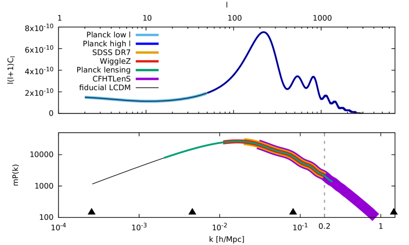
Figure 1: Comoving scales covered by the experiments used in our analysis. The vertical dashed line show the limit of the linear scales. The triangles show the position of the knots. The leftmost one is not visible in the plot.

We use a comprehensive set of power spectra obtained from observations of CMB and of large scale structure (including both weak gravitational lensing and galaxies redshift surveys) as follows:

• Planck power spectra of temperature and polarisation of the CMB. The Planck collaboration released in 2013 the temperature data from the first half of the mission [29]. We complement the Planck 2013 data with the WMAP polarisation. We refer to this as PlanckCMB13. In 2015 the results of the full analysis has been released [30]. Temperature and E-mode polarisation power spectra (and their cross-correlation) data and likelihoods come in two sets: a low $\ell$ from $\ell=2$ to $\ell=49$, and the high $\ell$ angular power spectrum. We use the temperature and polarisation data up to $\ell=2500$ and we refer to this as PlanckCMB15.

• Beside the CMB power spectrum, Planck reconstructed the CMB lensing potential [31], which contains information on the amplitude of large scale structure integrated from recombination to present time. We will refer to it as PlanckLens.

• The Canada-France-Hawaii Lensing Survey (CFHTLenS) [32] provides the two point correlation function of the tomographic weak lensing signal.

• The WiggleZ Dark Energy Survey (WiggleZ), through the measurement of position and redshift of 238,000 galaxies, mapped a volume of one cubic gigaparsec over seven regions of the sky up to a redshift $z\lesssim 1$. The corresponding galaxy power spectrum is presented in [33].

• The Sloan Digital Sky Survey collaboration, in Data release 7 (SDSS DR7), used a sample of luminous red galaxies to reconstruct the halo density field and its power spectrum roughly between $k=0.02$ $h$/Mpc and $k=0.2$ $h$/Mpc [34].

In figure 1 we show the scales probed by each experiment along with the location of the knots.

2.3 Runs set-up

We now describe the cross validation set up. In order to constrain both the shape of the PPS and the cosmological parameters, we have to consider CMB primary data in all CV runs. Because of time constraints PlanckCMB2013 is used in the set up CV runs but PlanckCMB2015 is used in the final run. This choice is conservative, favouring slightly more freedom (lower penalty) to the reconstructed PPS. Besides these, we have 4 other experiments: 2 measuring weak lensing and 2 using galaxy catalogues. We perform 3 CV runs in a pyramidal scheme as summarised in table 1. We start performing in parallel two different cross-validation analysis on two pairs of experiments where each pair is formed by a weak lensing experiment and by a galaxy catalogue. The dependence of the CV score on $\alpha_{p}$ was mapped by sampling several $\alpha_{p}$ values. The results of these preliminary runs show no unexpected behaviour or tension, i.e., the reconstructed PPS shows no significant deviation from a power-law, and the shape of the CV score is the same for both run 1.1 and run 1.2. Knowing this, we then combine the large scale structure data to have one weak lensing and one galaxy survey in each CV set. The best roughness penalty found from this CV is used in the final run which includes all experiments (this is called “Rec.” run in the table). The penalty parameter value to use in the reconstruction is determined by the CV score of run 2 alone: its dependence on $\alpha_{p}$ is illustrated in figure 2. The fact that the shape of the three CV scores — from run 1.1, 1.2, and 2 — shown in figure 2 is very similar, indicate robustness and that there are no significant tensions between the datasets.

Run	$A$	$B$
1.1	PlanckCMB13, PlanckLens	PlanckCMB13, SDSS DR7
1.2	PlanckCMB13, CFHTLenS	PlanckCMB13, WiggleZ
2	PlanckCMB13, PlanckLens, SDSS DR7	PlanckCMB13, CFHTLenS, WiggleZ
Rec.	PlanckCMB15, PlanckLens, SDSS DR7, CFHTLenS, WiggleZ

Table 1: Cross-validation datasets A and B for the various runs. The reconstruction (Rec.) involve all the experiments together.

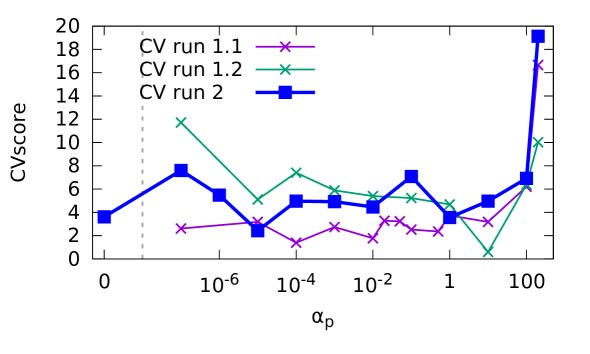
Figure 2: CV score as a function of $\alpha_{p}$ for the cross-validation run 2. A different arbitrary offset has been subtracted from each CV score.

The CV score has a fairly well defined “wall” for high penalties , but is quite constant under a certain threshold at $\alpha_{p}\sim 10$. For high $\alpha_{p}$ the penalty starts being the dominant contribution to the likelihood, so the behaviour in the limit of high $\alpha_{p}$ is expected. On the other hand, if small values of the penalty were to lead to overfitting, the CV score should increase as $\alpha_{p}$ decreases. This is not what we see and can be understood as follows. CMB angular power spectra are always included in the analysis and in this limit, it is the statistical power of these data (not the penalty) that drives the smoothness of the reconstruction and therefore the CV score. In other words, for low values of the penalty below $\alpha_{p}\sim 10$, all datasets are well consistent with the Planck-inferred PPS reconstruction: the CMB data alone disfavour unnecessarily wiggly shapes, even when there is a low penalty.

Since there is not a well defined minimum for the CV score, we opt for presenting two different cases. One is more conservative, in the sense that it has a stronger penalty that allows only small deviations from the concordance power-law model. For this one we choose $\alpha_{p}=1$.

The other leaves more freedom to the data, as we choose a more relaxed penalty $\alpha_{p}=0.01$. A reconstruction with $\alpha_{p}\ll 0.01$ is pretty much uninformative. In fact recall that the free parameters in our MCMC runs are the physical baryon density $\omega_{b}$, the physical cold dark matter density $\omega_{\rm{cdm}}$, the rescaled Hubble parameter $h$, the optical depth to reionization $\tau_{\rm{reio}}$, and the value of the five knots of the spline that we used to parametrize the shape of the PPS. At such low penalty values the reconstruction transfers in part the features of the radiation transfer function and the effect of the optical depth to reionization into the PPS opening up degeneracies in parameter space.

3 Results

Here we present the results with the latest Planck likelihood (2015 release) and all the large scale structure power spectrum data (Planck Lensing 2015, WiggleZ, CFHTLenS, and SDSS DR7), with the two different roughness penalties ($\alpha_{p}=1$ and $\alpha_{p}=0.01$) justified above.

As discussed in refs. [17, 35, 36, 37, 38] there is a tension between the inferred matter power spectrum amplitude from CMB and from CFHTLenS, which may arise from possible systematic errors in the photometric redshifts of CFHTLens. For this reason we present results first without and then with CFHTLens.

3.1 Reconstruction without CFHTLens

In figure 3(a) and 3(b) we show the reconstructed PPS for $\alpha_{p}=1$ and $\alpha_{p}=0.01$ respectively. The colour-bars on the upper side show the scales probed by each experiment as in figure 1, green for PlanckLens, red for WiggleZ, gold for SDSS DR7. PlanckCMB15 covers the whole plot. The best fit reconstruction is shown in yellow and errors are shown by plotting in dark blue (light blue) a random sample of 400 reconstructions chosen among the 68.27% most likely points (points in the range 68.27% - 95.45%) in the MCMC. The 95.5% confidence regions appear to coincide with the 68.3%: this is because the reconstructed spectra are simply more wiggly and are not allowed to deviate more, and consistently across scales, from the best fit.

In the figure the red and pale red regions show the 68 and 95% confidence intervals for the standard power law $\Lambda$CDM Planck 2015 TT, TE, EE + Low P analysis [2].

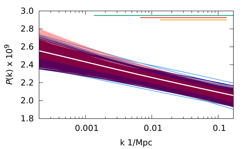
(a) $\alpha_{p}=1$.

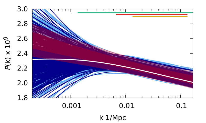
(b) $\alpha_{p}=0.01$.

Figure 3: Reconstructed PPS. The best fit reconstruction is shown in white. Errors are shown by plotting in dark blue (light blue) 400 spline picked at random among the 68.27% most likely points (points in the range 68.27% - 95.45%) in the MCMC. The red (pale red) region shows the 68% (95%) confidence intervals for Planck 2015 TT, TE, EE + Low P. The colour-bars on the upper side show the scales probed by each experiment as in figure 1, green for PlanckLens, red for WiggleZ, gold for SDSS DR7. PlanckCMB15 covers the whole plot.

Note that for the more conservative choice of the penalty, errors of the reconstructed PPS are comparable with errors from Planck parametric fit at all scales. For the less conservative penalty this is also true on scales corresponding to $\ell>30$. This did not happen with the previous generation of cosmological data (see [9]) where the reconstructed PPS was significantly less constrained than with a power law fit.

The additional freedom in the PPS allowed by the lower penalty $\alpha_{p}=0.01$ is used on scales corresponding to low CMB multipoles $\ell<30$. These scales are dominated by cosmic variance and are known to be lower than the standard $\Lambda$CDM prediction e.g., [29, 39, 40, 41] and refs therein.

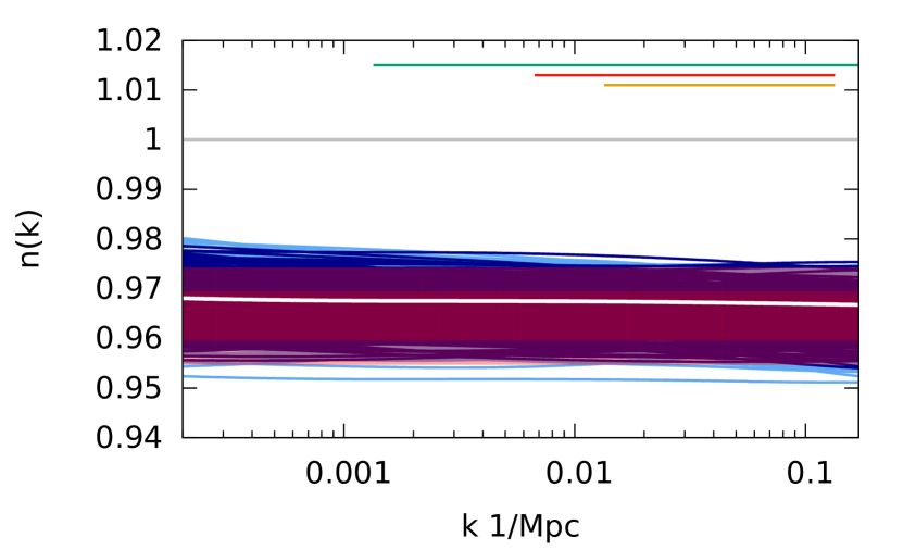
(a) $\alpha_{p}=1$.

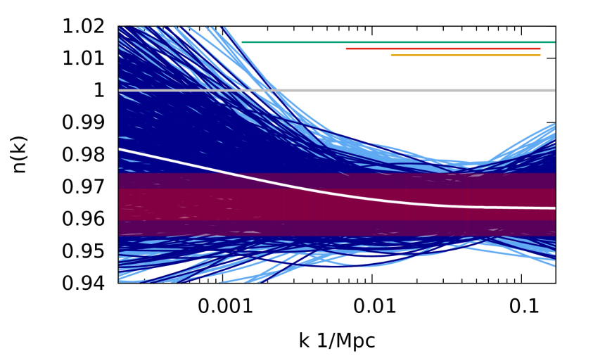
(b) $\alpha_{p}=0.01$.

Figure 4: Power spectrum spectral index of the reconstructed PPSs. The white line corresponds to the best fit reconstruction. Errors are shown by plotting in dark blue (light blue) 400 reconstructions randomly selected from the 68.27% most likely points (points in the range 68.27% - 95.45%) in the MCMC. The red (pale red) region shows 68% (95%) confidence intervals for the power law Planck 2015 TT, TE, EE + Low P fit. The colour-bars on the upper side show the scales probed by each experiment as in figure 1, green for PlanckLens red for WiggleZ, gold for SDSS DR7. PlanckCMB15 covers the whole plot. In the right figure, the grey line is $n(k)\equiv 1$, i.e., scale invariance.

In figure 4(a) and 4(b) we also show the reconstructed $n(k)\equiv d\ln P(k)/d\ln k$ ($\alpha_{p}=1$ and $\alpha_{p}=0.01$) for ease of comparison with the standard power law results. We find no evidence that any scale dependence of the power spectrum spectral slope is necessary, which is in agreement with previous analyses. However with this new data set we find that $n=1$ is highly disfavoured by the data, in particular for $\alpha_{p}=1$ the significance of the departure from scale invariance is comparable with that obtained when adopting the “inflation–motivated” power-law prior. Even for the more flexible reconstruction, not even one point of the more than $4\times 10^{5}$ MCMC points falls near scale invariance.

The results shown in Figs. 3 and 4 offer a powerful confirmation of the inflationary paradigm, justify the adoption of the inflationary prior in cosmological analyses.

Finally in figs. 5(a) and 5(b) we show the ratio of the reconstructed PPS to the best fit Planck 2015 (temperature, polarisation, and lensing) power law model.

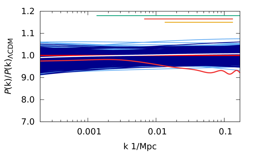
(a) $\alpha_{p}=1$.

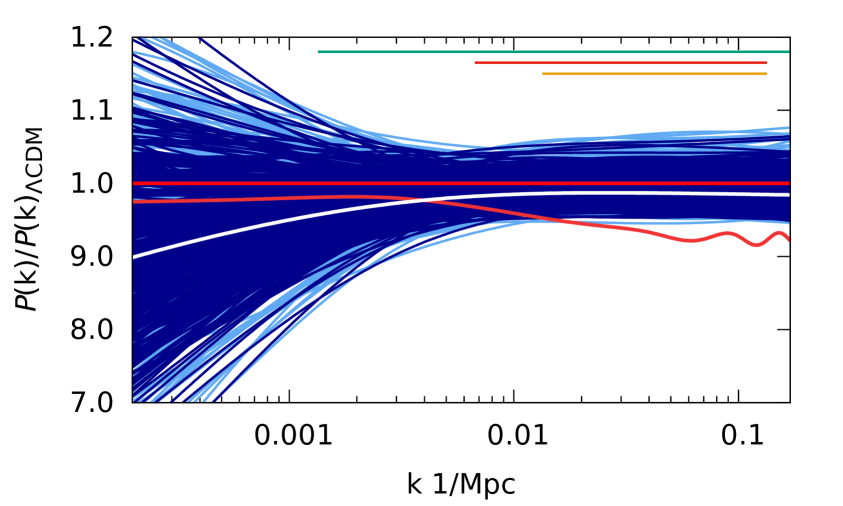
(b) $\alpha_{p}=0.01$.

Figure 5: Reconstructed PPS divided by the Planck 2015 TT, TE, EE + LowP + Lensing power-law PPS best-fit using the same conventions as Figs.3 for the legend and the reconstructed $P(k)$. The red lines show the small-scales power suppression effect due to massive neutrinos. The upper line is the $\Sigma m_{\nu}=0$ eV theoretical prediction based on the conditional best fit to Planck 2015 TT, TE, EE + Low P + Lensing + BAO + JLA + $H_{0}$ data, the lower line is the same with $\Sigma m_{\nu}=0.2$ eV.

The reconstruction is fully compatible with the parametric fit. The figure also shows the expected effect of small scale power suppression due to massive neutrino free-streaming for two representative values of neutrino masses $\Sigma m_{\nu}=0$ eV and $0.2$ eV. The two models are the conditional (i.e., keeping $\Sigma m_{\nu}$ fixed at the required value) best fit to the data (Planck 2015 TT, TE, EE + Low P + Lensing + BAO + JLA + $H_{0}$ data). Clearly models with $\Sigma m_{\nu}>0.2$ eV are highly disfavoured by the data even with this minimally parametric reconstruction: not a single step of a $4\times 10^{5}$ size MCMC goes near the $\Sigma m_{\nu}=0.2$ eV line. This of course does not exclude the — admittedly contrived — case with a arbitrarily large neutrino mass inducing a small scale power suppression which is cancelled by a compensating boost of the PPS on the same scales. Occam’s razor disfavours this scenario.

3.2 Reconstruction with CFHTLens

The reconstructed $P(k)$, $n(k)$ and $P(k)$ relative to the power law best fit are shown in figures 6, 7, and 8 using the same conventions as in figures 3, 4, and 5.

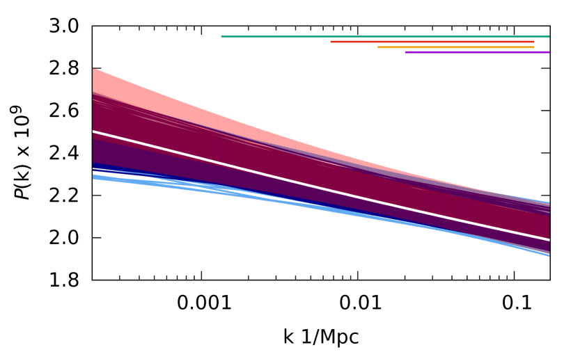
(a) $\alpha_{p}=1$.

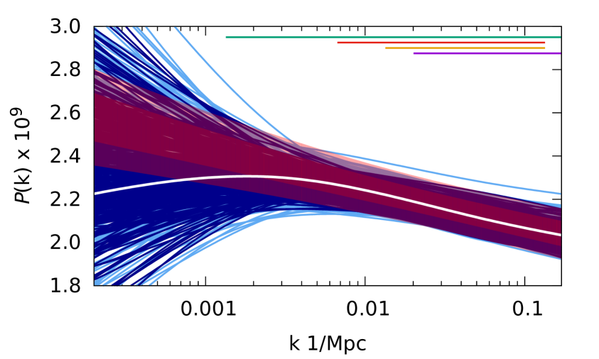
(b) $\alpha_{p}=0.01$.

Figure 6: Reconstructed PPS. Refer to figure 3 for explanation and colour code. In addition, the purple line shows the scales covered by CFHTLenS.

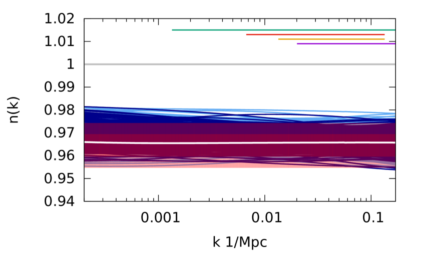
(a) $\alpha_{p}=1$.

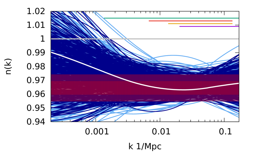
(b) $\alpha_{p}=0.01$.

Figure 7: Power spectrum spectral index of the reconstructed PPSs. Refer to figure 4 for explanation and colour code. In addition, the purple line shows the scales covered by CFHTLenS.

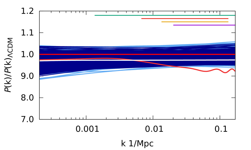
(a) $\alpha_{p}=1$.

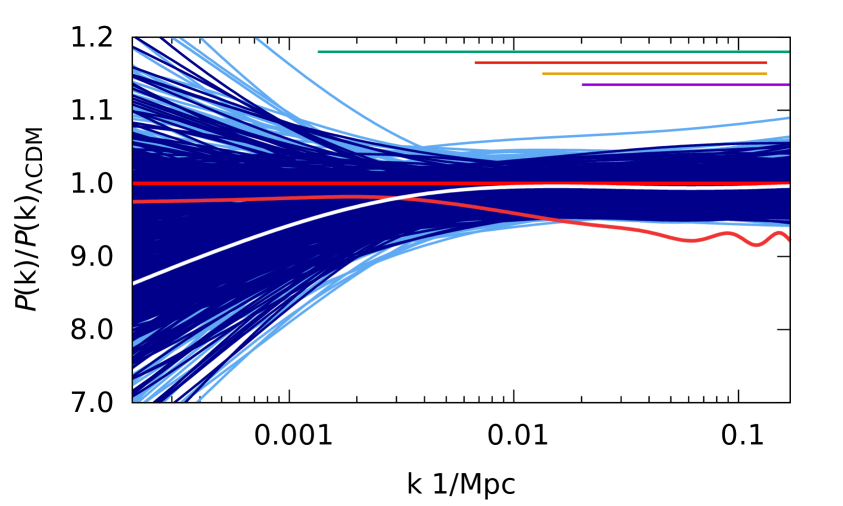
(b) $\alpha_{p}=0.01$.

Figure 8: Reconstructed PPS relative to Planck 2015 TT, TE, EE + LowP + Lensing power-law PPS best-fit. Refer to figure 5 for explanation and colour code. In addition, the purple line shows the scales covered by CFHTLenS.

Comparison with the results of section 3.1 (in figures 3, 4, 5) shows that qualitatively the reconstructions are very similar, there is no strong evidence for deviations from the power law behaviour and scale invariance is still excluded. However quantitatively some differences may be appreciated. Adding the CFHTLenS datasets has the effect of lowering the overall PPS normalisation (clearly visible by comparison with figure 3).

The ratio with Planck power law best-fit in figure 8 highlights how, independently from our choice of datasets, high neutrino masses are disfavoured. Quantitatively the $\Sigma m_{\nu}>0.2$ eV bound is excluded at more than 95% confidence if we assume a power law PPS, as discussed in section 3.1.

For completeness we also report the recovered values and errors for all the model parameters in table 2 and table 3 for the two penalties $\alpha_{p}=1$ and $\alpha_{p}=0.01$ respectively.

Without CFHTLenS $\qquad-\ln{\cal L}_{\mathrm{min}}=6727.02$
Param	best-fit	mean$\pm\sigma$	95% lower	95% upper
$100\leavevmode\nobreak\ \omega_{b}$	$2.226$	$2.229_{-0.015}^{+0.015}$	$2.199$	$2.258$
$\omega_{\rm{cdm}}$	$0.1194$	$0.1191_{-0.0011}^{+0.0011}$	$0.1168$	$0.1214$
$h$	$0.6795$	$0.6815_{-0.0053}^{+0.0052}$	$0.6712$	$0.6919$
$\tau$	$0.0542$	$0.05982_{-0.013}^{+0.0092}$	$0.04001$	$0.07955$
$10^{+9}K_{1}$	$2.788$	$2.736_{-0.12}^{+0.11}$	$2.507$	$2.965$
$10^{+9}K_{2}$	$2.546$	$2.534_{-0.07}^{+0.07}$	$2.395$	$2.673$
$10^{+9}K_{3}$	$2.307$	$2.32_{-0.049}^{+0.043}$	$2.231$	$2.412$
$10^{+9}K_{4}$	$2.072$	$2.108_{-0.053}^{+0.036}$	$2.028$	$2.194$
$10^{+9}K_{5}$	$1.872$	$1.9_{-0.059}^{+0.047}$	$1.802$	$2.006$
With CFHTLenS $\qquad-\ln{\cal L}_{\mathrm{min}}=6777.64$
Param	best-fit	mean$\pm\sigma$	95% lower	95% upper
$100\leavevmode\nobreak\ \omega_{b}$	$2.244$	$2.236_{-0.014}^{+0.015}$	$2.207$	$2.264$
$\omega_{\rm{cdm}}$	$0.1182$	$0.1182_{-0.001}^{+0.0011}$	$0.1161$	$0.1204$
$h$	$0.6867$	$0.6854_{-0.0051}^{+0.0048}$	$0.6757$	$0.6953$
$\tau$	$0.05239$	$0.05852_{-0.013}^{+0.0087}$	$0.04001$	$0.07795$
$10^{+9}K_{1}$	$2.721$	$2.697_{-0.12}^{+0.12}$	$2.463$	$2.931$
$10^{+9}K_{2}$	$2.512$	$2.504_{-0.071}^{+0.069}$	$2.363$	$2.645$
$10^{+9}K_{3}$	$2.281$	$2.3_{-0.048}^{+0.041}$	$2.213$	$2.389$
$10^{+9}K_{4}$	$2.065$	$2.098_{-0.051}^{+0.035}$	$2.021$	$2.182$
$10^{+9}K_{5}$	$1.869$	$1.9_{-0.058}^{+0.045}$	$1.802$	$2.003$

Table 2: Best fit, mean and confidence intervals for the MCMC parameters in the reconstruction with $\alpha_{p}=1$

Without CFHTLenS $\qquad-\ln{\cal L}_{\mathrm{min}}=6726.32$
Param	best-fit	mean$\pm\sigma$	95% lower	95% upper
$100\leavevmode\nobreak\ \omega_{b}$	$2.239$	$2.226_{-0.016}^{+0.016}$	$2.194$	$2.259$
$\omega_{\rm{cdm}}$	$0.1173$	$0.1193_{-0.0012}^{+0.0013}$	$0.1168$	$0.1218$
$h$	$0.6898$	$0.6806_{-0.006}^{+0.0055}$	$0.6694$	$0.6922$
$\tau$	$0.07136$	$0.05974_{-0.014}^{+0.0088}$	$0.04$	$0.08061$
$10^{+9}K_{1}$	$1.968$	$2.351_{-0.69}^{+0.67}$	$1.014$	$3.711$
$10^{+9}K_{2}$	$2.159$	$2.351_{-0.3}^{+0.29}$	$1.769$	$2.934$
$10^{+9}K_{3}$	$2.272$	$2.31_{-0.062}^{+0.059}$	$2.191$	$2.431$
$10^{+9}K_{4}$	$2.148$	$2.106_{-0.056}^{+0.036}$	$2.024$	$2.198$
$10^{+9}K_{5}$	$1.933$	$1.923_{-0.078}^{+0.073}$	$1.773$	$2.074$
With CFHTLenS $\qquad-\ln{\cal L}_{\mathrm{min}}=6776.95$
Param	best-fit	mean$\pm\sigma$	95% lower	95% upper
$100\leavevmode\nobreak\ \omega_{b}$	$2.235$	$2.234_{-0.016}^{+0.015}$	$2.203$	$2.266$
$\omega_{\rm{cdm}}$	$0.1179$	$0.1182_{-0.0011}^{+0.0012}$	$0.116$	$0.1205$
$h$	$0.686$	$0.6853_{-0.0054}^{+0.0052}$	$0.6749$	$0.6958$
$\tau$	$0.06203$	$0.05911_{-0.014}^{+0.0085}$	$0.04$	$0.07976$
$10^{+9}K_{1}$	$2.241$	$2.42_{-0.69}^{+0.67}$	$1.09$	$3.784$
$10^{+9}K_{2}$	$2.294$	$2.373_{-0.31}^{+0.28}$	$1.787$	$2.962$
$10^{+9}K_{3}$	$2.28$	$2.292_{-0.063}^{+0.056}$	$2.176$	$2.414$
$10^{+9}K_{4}$	$2.106$	$2.1_{-0.055}^{+0.035}$	$2.019$	$2.189$
$10^{+9}K_{5}$	$1.899$	$1.919_{-0.08}^{+0.071}$	$1.772$	$2.071$

Table 3: Best fit, mean and confidence intervals for the MCMC parameters in the reconstruction with $\alpha_{p}=0.01$

The degeneracies among the parameters for the PPS value at the knots can be appreciated in the triangle plots of figure 9(a) for $\alpha_{p}=1$ and figure 9(b) for $\alpha_{p}=0.01$. Correlations with and among the cosmological parameters not shown are negligible. As expected, higher penalty induce correlations among the knots which are stronger between neighbouring ones.

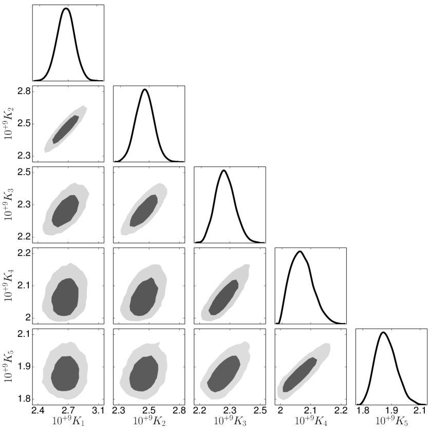
(a) $\alpha_{p}=1$.

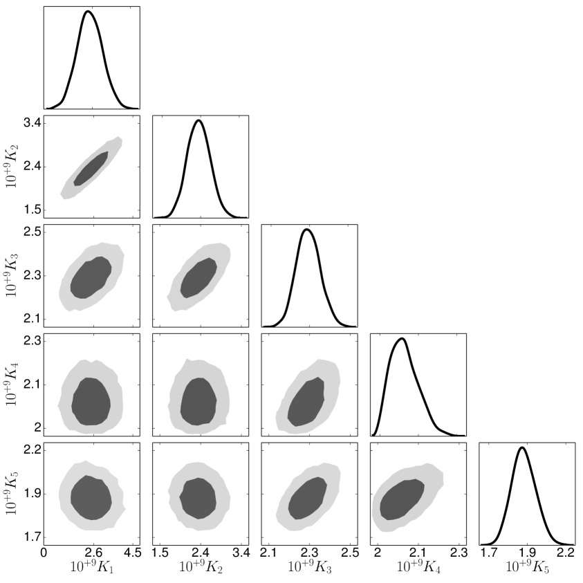
(b) $\alpha_{p}=0.01$.

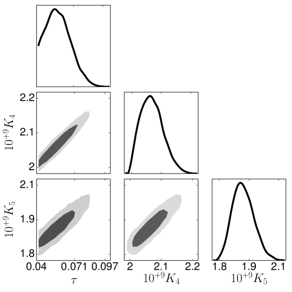
(c) $\alpha_{p}=1$.

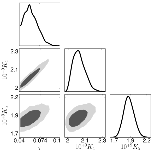
(d) $\alpha_{p}=0.01$.

Figure 9: Triangular plots for the run with all the datasets combined. We refer to the value of the spline function evaluated at the $i$-th knot as $K_{i}$.

Interestingly the only cosmological parameter that correlates with the knots is $\tau_{\rm{reio}}$, which show degeneracy with the knots at higher $k$ (figure 9(c) and 9(d)). This behaviour is however not unexpected. The $\tau_{\rm{reio}}$ parameter only affects the CMB and in particular its main effect is to suppress the temperature power spectrum at multipoles $\ell\gtrsim 80$. With our choice for the location of the knots, the most affected knots are therefore $K_{4}$ and $K_{5}$. Improved polarisation data at low $\ell$ should reduce this degeneracy. The figure excluding the CFHTLenS dataset is qualitatively very similar and thus is not shown here.

4 Discussion and conclusions

The analysis of the latest cosmological data [2] indicates a highly significant deviation from scale invariance of the primordial power spectrum (PPS) when parameterized by a power law or by a spectral index and a “running”. This offers a powerful tool to discriminate among theories for the origin of perturbations and among inflationary models. In fact, the deviation from scale invariance of the PPS is a critical prediction of inflation and is the only signature that is generic to all inflationary models. It is therefore a vital test of the inflationary paradigm.

One may wonder if a strong theory prior on the form of the power spectrum, such as the power law prescription, can lead to artificially tight constraints or even a spurious detection of a deviation from scale invariance, if the adopted model were not a good fit to the data.

Here we have built on the work of [7, 8] to reconstruct the PPS with a minimally parametric approach, using the cross-validation technique as the smoothness criterion. We consider a comprehensive set of state-of-the art cosmological data including probes of the Cosmic Microwave Background, and of large scale structure via gravitational lensing and galaxy redshift surveys. While the spline reconstruction used here is best suited for smooth features in the PPS, it is also sensitive to sharp features if they have high enough signal-to-noise.

We find that there is no evidence for deviations from a power law PPS, and that errors of the reconstructed PPS are comparable with errors obtained with a power law fit. These results should be compared with those presented in [9], to appreciate the increase in statistical power brought about by the latest generation of experiments. In fact with current data a scale-invariant power spectrum is highly disfavoured even with this minimally parametric reconstruction. In particular for our conservative choice of smoothness penalty parameter values the significance of the departure from scale invariance is comparable with that obtained when adopting the “inflation–motivated” power-law prior. Constraints no longer relax significantly when generic forms of the PPS are allowed.

Because of its flexibility, our reconstruction would be able to detect the tell-tale signature of small scale power suppression induced by free streaming of neutrino if they are sufficiently massive. Of course in reality the suppression happens in the late-time power spectrum, not in the primordial one. But as we do not include the effect of neutrino masses in the matter transfer function, the reconstruction would recover an “effective” small scale damping. Our reconstruction detects no such signature, ruling out a model with a power law PPS and sum of neutrino masses of $0.2$ eV or larger.

Our results, which recover in a model independent way a power law power spectrum with a small but highly significant red tilt, offer a powerful confirmation of the inflationary paradigm, justifying adoption of the inflationary prior in cosmological analyses.

Appendix: Reconstruction sensitivity to non-primordial effects

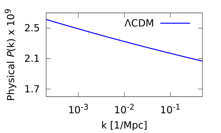
A.1 In the first case the initial condition is a power-law PPS.

B.1 In the second case the neutrino damping is considered in the initial conditions.

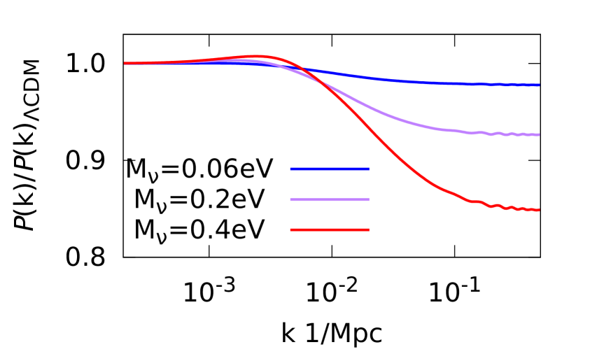
A.2 Then the evolution takes into account the presence of massive neutrino.

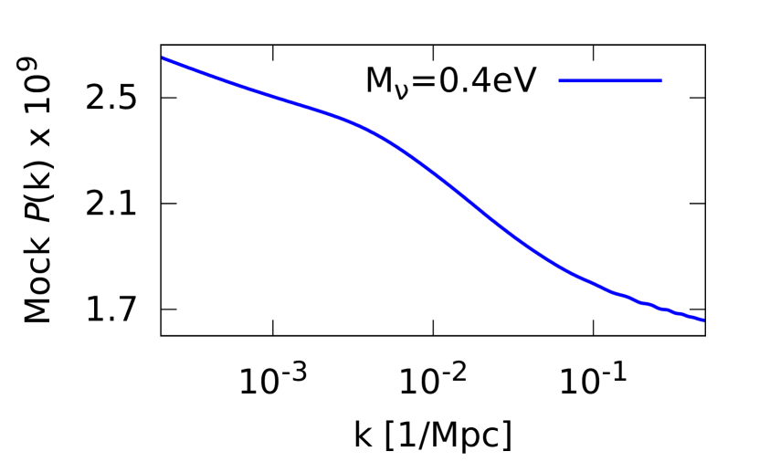
B.2 The initial condition is a power-law multiplied by the neutrino power suppression. Then the evolution equation with massless neutrino is used.

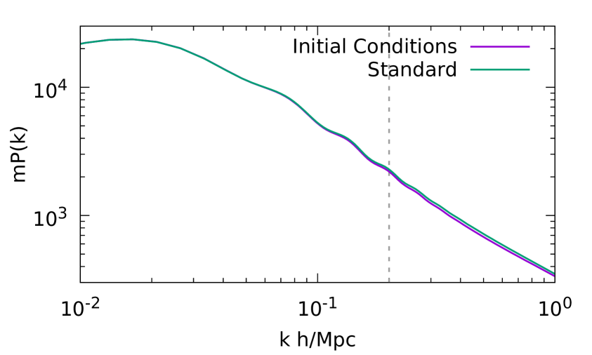
R.1 The two methods generate the same observables in the scales of interest. Here we show the non-linear matter power spectrum.

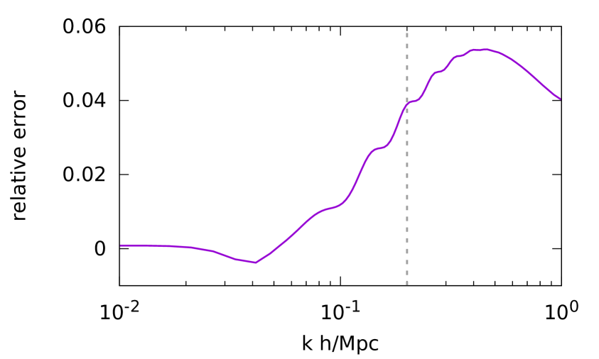
R.2 The error do not exceed 1% at scales larger than $k=0.1$ $h/$Mpc and is due to non-linearities.

Figure 10: How a non-zero neutrino mass would induce a power suppression in the reconstructed power spectrum. Both method 10A.1–10A.2 and 10B.1–10B.2 give the same result 10R.1–10R.2 at linear level.

Figure 10A.1–10R.2 visualises the concept — exploited here — that in the reconstructed power spectrum the effect of a non-zero neutrino mass is degenerate with a power suppression. This is a good approximation especially on scales where the evolution is linear or mildly non-linear, i.e., $k\leavevmode\nobreak\ <\leavevmode\nobreak\ 0.2\leavevmode\nobreak\ \ \leavevmode\nobreak\ h$/Mpc. Consider a $\Lambda$CDM universe with massive neutrinos, where all the cosmological parameters are known and with a power law PPS at the end of inflation (figure 10A.1). From these initial conditions we evolve the perturbations assuming massive neutrino (different values for the total mass are shown). On small physical scales neutrino free streaming [42] suppresses power 10A.2) yielding a resulting power spectrum shown in figure 10R.1. Now we can think of an alternative method: implement the neutrino power suppression (figure 10B.1) directly on the initial PPS as a deviation from a power law as shown in figure 10B.2. This initial power spectrum is then evolved assuming massless neutrinos. The linearity of the perturbation evolution equations guarantees that the generated matter and CMB power spectra would be the same as in the first case (figure 10R.1). In figure 10R.2 we can appreciate the fact that discrepancies in the prediction made in the two cases come from non-linearities. For example, when considering neutrino with $\Sigma m_{\nu}=0.4$ eV we expect a small scale suppression in the linear power spectrum of 15% (figure 10A.2). The differences due to non linearities exceed 1% only above $k=0.1$ $h/$Mpc, and are never more than 4% at the scales of interest. This means that in principle this approach we should be able to distinguish the effect for $\Sigma m_{\nu}\geq 0.06$ eV, even though it would prevent us to obtain an unbiased measure in case of detection.

Another source of error that might contribute is given by the use of spline with a limited number of knots. If the number of knots, or their position, is not suitably chosen, one could be unable to reconstruct a given signal. It is not our case, with our choice of knots we have verified that we can reconstruct any neutrino power suppression with a $10^{-3}$ accuracy.

References

- [1] Planck Collaboration, P. A. R. Ade, N. Aghanim, et al., Planck 2013 results. I. Overview of products and scientific results, Astronomy & Astrophysics 571 (Nov., 2014) A1, [arXiv:1303.5062].
- [2] Planck Collaboration, P. A. R. Ade, N. Aghanim, et al., Planck 2015 results. XIII. Cosmological parameters, ArXiv e-prints (Feb., 2015) [arXiv:1502.01589].
- [3] V. Miranda and W. Hu, Inflationary steps in the Planck data, Physical Review D 89 (Apr., 2014) 083529, [arXiv:1312.0946].
- [4] P. D. Meerburg, D. N. Spergel, and B. D. Wandelt, Searching for oscillations in the primordial power spectrum. II. Constraints from Planck data, Physical Review D 89 (Mar., 2014) 063537, [arXiv:1308.3705].
- [5] X. Chen, M. H. Namjoo, and Y. Wang, Models of the Primordial Standard Clock, Journal of Cosmology and Astroparticle Physics 2 (Feb., 2015) 27, [arXiv:1411.2349].
- [6] U. H. Danielsson, Note on inflation and trans-Planckian physics, Physical Review D 66 (July, 2002) 023511, [hep-th/0203198].
- [7] C. Sealfon, L. Verde, and R. Jimenez, Smoothing spline primordial power spectrum reconstruction, Physical Review D 72 (nov, 2005) 103520, [astro-ph/0506707].
- [8] L. Verde and H. Peiris, On minimally parametric primordial power spectrum reconstruction and the evidence for a red tilt, Journal of Cosmology and Astroparticle Physics 7 (July, 2008) 9, [arXiv:0802.1219].
- [9] H. V. Peiris and L. Verde, The shape of the primordial power spectrum: A last stand before Planck data, Physical Review D 81 (Jan., 2010) 021302, [arXiv:0912.0268].
- [10] Planck Collaboration, P. A. R. Ade, N. Aghanim, et al., Planck 2015 results. XX. Constraints on inflation, ArXiv e-prints (Feb., 2015) [arXiv:1502.02114].
- [11] L. Verde, P. Protopapas, and R. Jimenez, Planck and the local universe: Quantifying the tension, Physics of the Dark Universe 2 (2013), no. 3 166 – 175.
- [12] R. A. Battye and A. Moss, Evidence for massive neutrinos from cosmic microwave background and lensing observations, Phys. Rev. Lett. 112 (Feb, 2014) 051303.
- [13] M. Wyman, D. H. Rudd, R. A. Vanderveld, and W. Hu, Neutrinos help reconcile planck measurements with the local universe, Phys. Rev. Lett. 112 (Feb, 2014) 051302.
- [14] J. Hamann and J. Hasenkamp, A new life for sterile neutrinos: resolving inconsistencies using hot dark matter, Journal of Cosmology and Astroparticle Physics 2013 (2013), no. 10 044.
- [15] F. Beutler, S. Saito, J. R. Brownstein, et al., The clustering of galaxies in the SDSS-III Baryon Oscillation Spectroscopic Survey: signs of neutrino mass in current cosmological data sets, Monthly Notices of the Royal Astronomical Society 444 (Nov., 2014) 3501–3516, [arXiv:1403.4599].
- [16] E. Giusarma, E. Di Valentino, M. Lattanzi, A. Melchiorri, and O. Mena, Relic neutrinos, thermal axions, and cosmology in early 2014, Physical Review D 90 (Aug., 2014) 043507, [arXiv:1403.4852].
- [17] Planck Collaboration, P. A. R. Ade, N. Aghanim, et al., Planck 2013 results. XVI. Cosmological parameters, Astronomy & Astrophysics 571 (Nov., 2014) A16, [arXiv:1303.5076].
- [18] S. M. Feeney, H. V. Peiris, and L. Verde, Is there evidence for additional neutrino species from cosmology?, Journal of Cosmology and Astroparticle Physics 2013 (2013), no. 04 036.
- [19] J.-W. Hu, R.-G. Cai, Z.-K. Guo, and B. Hu, Cosmological parameter estimation from cmb and x-ray cluster after planck, Journal of Cosmology and Astroparticle Physics 2014 (2014), no. 05 020.
- [20] L. Verde, S. M. Feeney, D. J. Mortlock, and H. V. Peiris, (lack of) cosmological evidence for dark radiation after planck, Journal of Cosmology and Astroparticle Physics 2013 (2013), no. 09 013.
- [21] G. Efstathiou, H0 revisited, Monthly Notices of the Royal Astronomical Society 440 (May, 2014) 1138–1152, [arXiv:1311.3461].
- [22] B. Leistedt, H. V. Peiris, and L. Verde, No New Cosmological Concordance with Massive Sterile Neutrinos, Physical Review Letters 113 (July, 2014) 041301, [arXiv:1404.5950].
- [23] A. J. Cuesta, V. Niro, and L. Verde, Neutrino mass limits: robust information from the power spectrum of galaxy surveys, Physics of the Dark Universe (2016) [arXiv:1511.05983].
- [24] N. Palanque-Delabrouille, C. Yèche, J. Baur, et al., Neutrino masses and cosmology with Lyman-alpha forest power spectrum, Journal of Cosmology and Astroparticle Physics 11 (Nov., 2015) 011, [arXiv:1506.05976].
- [25] P. Green and B. Silverman, Nonparametric regression and generalized linear models: a roughness penalty approach. Chapman & Hall, 1994.
- [26] D. Blas, J. Lesgourgues, and T. Tram, The Cosmic Linear Anisotropy Solving System (CLASS). Part II: Approximation schemes, Journal of Cosmology and Astroparticle Physics 7 (July, 2011) 34, [arXiv:1104.2933].
- [27] B. Audren, J. Lesgourgues, K. Benabed, and S. Prunet, Conservative Constraints on Early Cosmology: an illustration of the Monte Python cosmological parameter inference code, JCAP 1302 (2013) 001, [arXiv:1210.7183].
- [28] S. Dodelson, Modern Cosmology. Academic Press, 2003.
- [29] Planck Collaboration, P. A. R. Ade, N. Aghanim, et al., Planck 2013 results. XV. CMB power spectra and likelihood, Astronomy & Astrophysics 571 (Nov., 2014) A15, [arXiv:1303.5075].
- [30] Planck Collaboration, N. Aghanim, M. Arnaud, et al., Planck 2015 results. XI. CMB power spectra, likelihoods, and robustness of parameters, ArXiv e-prints (July, 2015) [arXiv:1507.02704].
- [31] Planck Collaboration, P. A. R. Ade, N. Aghanim, et al., Planck 2013 results. XVII. Gravitational lensing by large-scale structure, Astronomy & Astrophysics 571 (Nov., 2014) A17, [arXiv:1303.5077].
- [32] C. Heymans, L. Van Waerbeke, L. Miller, et al., CFHTLenS: the Canada-France-Hawaii Telescope Lensing Survey, Monthly Notices of the Royal Astronomical Society 427 (Nov., 2012) 146–166, [arXiv:1210.0032].
- [33] D. Parkinson, S. Riemer-Sørensen, C. Blake, et al., The WiggleZ Dark Energy Survey: Final data release and cosmological results, Physical Review D 86 (Nov., 2012) 103518, [arXiv:1210.2130].
- [34] B. A. Reid, W. J. Percival, D. J. Eisenstein, et al., Cosmological constraints from the clustering of the Sloan Digital Sky Survey DR7 luminous red galaxies, Monthly Notices of the Royal Astronomical Society 404 (May, 2010) 60–85, [arXiv:0907.1659].
- [35] N. MacCrann, J. Zuntz, S. Bridle, B. Jain, and M. R. Becker, Cosmic discordance: are Planck CMB and CFHTLenS weak lensing measurements out of tune?, Monthly Notices of the Royal Astronomical Society 451 (Aug., 2015) 2877–2888, [arXiv:1408.4742].
- [36] S. Joudaki, C. Blake, C. Heymans, et al., CFHTLenS revisited: assessing concordance with Planck including astrophysical systematics, ArXiv e-prints (Jan., 2016) [arXiv:1601.05786].
- [37] T. D. Kitching, L. Verde, A. F. Heavens, and R. Jimenez, Discrepancies between CFHTLenS cosmic shear and Planck: new physics or systematic effects?, Monthly Notices of the Royal Astronomical Society 459 (June, 2016) 971–981, [arXiv:1602.02960].
- [38] A. Choi, C. Heymans, C. Blake, et al., CFHTLenS and RCSLenS: Testing Photometric Redshift Distributions Using Angular Cross-Correlations with Spectroscopic Galaxy Surveys, ArXiv e-prints (Dec., 2015) [arXiv:1512.03626].
- [39] D. J. Schwarz, C. J. Copi, D. Huterer, and G. D. Starkman, CMB Anomalies after Planck, ArXiv e-prints (Oct., 2015) [arXiv:1510.07929].
- [40] C. J. Copi, D. Huterer, D. J. Schwarz, and G. D. Starkman, Lack of large-angle TT correlations persists in WMAP and Planck, Monthly Notices of the Royal Astronomical Society 451 (Aug., 2015) 2978–2985, [arXiv:1310.3831].
- [41] C. J. Copi, D. Huterer, D. J. Schwarz, and G. D. Starkman, Large-Angle Anomalies in the CMB, Advances in Astronomy 2010 (2010) 847541, [arXiv:1004.5602].
- [42] J. Lesgourgues and S. Pastor, Massive neutrinos and cosmology, Physics Reports 429 (July, 2006) 307–379, [astro-ph/0603494].