Positron surface state as a new spectroscopic probe for characterizing surfaces of topological insulator materials

Abstract

Topological insulators are attracting considerable interest due to their potential for technological applications and as platforms for exploring wide-ranging fundamental science questions. In order to exploit, fine-tune, control and manipulate the topological surface states, spectroscopic tools which can effectively probe their properties are of key importance. Here, we demonstrate that positrons provide a sensitive probe for topological states, and that the associated annihilation spectrum provides a new technique for characterizing these states. Firm experimental evidence for the existence of a positron surface state near Bi₂Te₂Se with a binding energy of $E_{b}=2.7\pm 0.2\,\text{eV}$ is presented, and is confirmed by first-principles calculations. Additionally, the simulations predict a significant signal originating from annihilation with the topological surface states and shows the feasibility to detect their spin-texture through the use of spin-polarized positron beams.

I Introduction

Quickly after their initial discovery, topological insulators (TIs) were recognized to hold significant potential for new technological applications and as playground for fundamental physics Hasan and Kane (2010); *Bansil2016; *Moore2010; *Mellnik2014; *Mourik2012. An intrinsic challenge with TIs, which arises due to the fact that their interesting properties originate from Dirac states located in a nanoscopic layer near the surface, remains to separate the fingerprint of the topological surface states from the bulk behaviour of the sample. Highly surface sensitive techniques such as angle resolved photoemission spectroscopy and scanning tunnelling microscopy have thus proven to be an indispensable tool to establish the existence of the gapless states in several systems and to confirm various of the predicted quasi-particle properties Hsieh et al. (2008); *Hsieh2009; *Roushan2009; *Xia2009.
In this article, we demonstrate that positrons provide a highly surface sensitive probe for the topological Dirac states. Since positron annihilation spectroscopy (PAS) techniques, with measurements of the 2D angular correlation of the annihilation radiation (2D-ACAR) in particular, are well suited to measure both the low and high momentum components of the annihilating electronic states without complication of matrix element effects, they can provide useful information on the Dirac state orbitals. Our calculations show that spin-polarized positron beams can additionally resolve the spin-textures associated with the topological states, owing to the predominant annihilation between particles with opposite spins Berko and Zuckerman (1964).
In section II, we present the experimental evidence for the existence of a bound positron state at the surface of the TI Bi₂Te₂Se and the measured binding energy Shastry et al. (2015). Section III contains a discussion of the theory and computational details used in our first principles investigation. In section IV, we show that the theory confirms the experimental interpretation and predicts a significant overlap between the positron and the topological states. We also demonstrate that spin-polarized positron measurements can reveal the spin-structure at the surface. In section V we summarize the results and discuss possible applications and advantages of PAS over other spectroscopic techniques.

II Experimental results

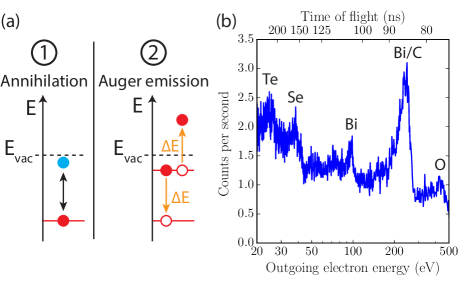
Figure 1: (a) Schematic representation of the PAES mechanism. In the first step, a positron (blue) annihilates with an electron (red) occupying a core level and creates a highly unstable hole. In the second step, an electron from a higher level fills this hole and transfers the energy difference between the two levels to a second electron. If the energy difference is sufficiently large, and the second electron is close enough to the surface, it can traverse the surface dipole and escape from the sample. The measured outgoing electron energy corresponds with the transferred energy in the Auger process minus the energy difference between the second electron’s state and the vacuum level. (b) Results of the PAES measurements on the Bi₂Te₂Se sample in which Auger signals from the different elements are indicated.

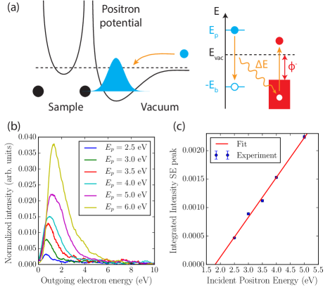
Figure 2: (a) Schematic representation of the AMPS mechanism. The left part of the diagram shows the incident positron (blue) that drops in the image potential well. In this process, the positron transfers an energy $\Delta E$, determined by the incident kinetic energy $E_{p}$ and the binding energy of the SS $E_{b}$, to an electron of the system through a virtual photon, as indicated in the right part of the figure. If the energy difference is larger than the electronic workfunction $\phi^{-}$, the electron can escape to the vacuum. (b) The measured low-energy Auger signals for the Bi₂Te₂Se sample. The outgoing electron energy is determined by the transferred energy $\Delta E$ minus the required energy to escape from the sample. The different lines show the result for varying energies of the incident positrons. (c) The integrated peak amplitudes of the low-energy Auger signal associated with the AMPS mechanism as a function of the incident positron energy.

Our Bi₂Te₂Se films are grown by molecular beam epitaxy on Si (111). The substrates are etched in hydrofluoric acid prior to loading in vacuum. A stoichiometric 2:2:1 Bi:Te:Se flux ratio is used. The substrate temperature is fixed at 200 ^∘C during the growth. The films used in this study are typically 40 nm thick. A 100 nm Se cap is then deposited, in-situ, on the sample surface after cooling down the substrate to room temperature. The capping layer protects the film surface from oxidation and atmospheric contaminants.
X-ray diffraction (XRD) is systematically used to characterize the samples, as briefly discussed in ref. Assaf et al., 2013. The c-axis lattice constant for the film used in this work is found to be equal to $30.10\pm 0.03~{}\text{\AA}$. Energy dispersive X-ray spectroscopy confirmed stoichiometry within a 5% error on samples resulting from an identical growth.
The samples are then transferred to the experimental positron chamber. In order to decap the samples, the protective Se layer is evaporated under UHV conditions, prior to the positron annihilation experiment. A heater button is placed behind the sample in a holder and a suitable current was passed to heat the sample for 20 minutes at 200 ^∘C. This procedure is similar to the decapping sequence used in ref. Zhang et al., 2012. The technical details concerning the setup of the positron experiments can be found in ref. Shastry et al., 2015 and references therein.
Positrons annihilate predominantly with the valence electrons but the small fraction that annihilates with core electrons produces highly unstable core holes, which are filled by the Auger process. Therefore, if positrons annihilate in a surface state (SS), positron-induced Auger-electron spectroscopy (PAES) provides a particularly clean method to determine the composition of the surface, free from a secondary electron background Weiss et al. (1988). A schematic picture of the process is drawn in figure 1(a). Results of PAES experiments from the TI Bi₂Te₂Se surface are shown in figure 1(b), where signals from Bi, Te, Se, C and O can be identified; the latter two are caused by the presence of a small concentration of contaminants adsorbed on the surface Shastry et al. (2015). These results reveal the presence of a bound positron SS. Were this not the case, positrons would either get trapped between the blocks of quintuple layers (QL) of the material or would be re-emitted before they annihilate. Since the extent of one QL block is about $10\,\text{\AA}$, which corresponds roughly to the mean free path of a $60\,\text{eV}$ electron, any Auger signal coming from below the first QL is too weak to be detected. Thus, the fact that the annihilation induced Auger peak intensities are observable is clear evidence that the positron is in a state localized at the surface at the time it annihilates.
Auger Mediated Positron Sticking (AMPS) experiments provide an independent proof for the existence of the SS and allow us to determine its binding energy Mukherjee et al. (2010). In the AMPS mechanism, the excess energy from a positron dropping into the image potential well is transferred to a valence electron. This can result in the emission of an Auger electron if the energy difference between the positron SS and the initial state, determined by the incident positron’s kinetic energy, is larger than the electron workfunction Mukherjee et al. (2010). The maximum kinetic energy of the Auger electrons is then given by $E_{max}=E_{p}+E_{b}-\phi^{-}$, where $E_{p}$ is the energy of the incident positron, $E_{b}$ is the binding energy of the positron surface state, and $\phi^{-}$ is the electron workfunction. Figure 2(a) illustrates the AMPS mechanism schematically. The observed increase in amplitude of the Auger signal at low energies as the energy of the incident positrons is increased, is shown in figure 2(b), and it confirms the presence of the SS. Knowing the electron workfunction, the binding energy of the SS can be determined from the positron energy threshold value for Auger electron emission: $E_{Th}=E_{p}$ for which $E_{max}=0$. The linear fit shown in figure 2(c), yields $E_{Th}=1.8\,\text{eV}$. Next, by considering the measured activation energy $E_{a}=0.4\,\text{eV}$ for positronium (Ps) desorption from the surface Shastry et al. (2015), one can eliminate the electron workfunction using the expression Chu et al. (1981), $E_{a}=E_{b}+\phi^{-}-6.80\,\text{eV}$, which gives a binding energy of $E_{b}=2.7\pm 0.2\,\text{eV}$ (ref. Shastry et al., 2015).

III Theory and computational details

Our first-principles calculations are carried out in the zero-positron-density limit of the two-component electron-positron density functional theory (2CDFT) Chakraborty and Siegel (1983); Boronski and Nieminen (1986). In this limit, which is exact in the case of a delocalized positron in a perfect crystal or at a surface, the electron density remains unperturbed by the presence of the positron. The computations thus consists of an electronic and positronic groundstate calculation which are performed subsequently.

III.1 Electronic structure

The electronic ground state is obtained using the projector-augmented wave (PAW) method Blöchl (1994) as implemented in the VASP software package Kresse and Furthmüller (1996a, b); Kresse and Joubert (1999). Electron exchange-correlation effects are treated using the Perdew-Burke-Ernzerhof (PBE) functional Perdew et al. (1996), and spin-orbit coupling is included in the computations. The kinetic energy cutoff for the plane-wave expansion of the wavefunctions is set to $275\,\text{eV}$. For the bulk calculations, we use the rhombohedral unit cell with a $\Gamma$-centered $11\times 11\times 11$ k-grid in combination with a Gaussian smearing of width $0.1\,\text{eV}$. In the surface calculations, we use a slab geometry with a vacuum of $15\,\text{\AA}$ to avoid spurious interactions between periodic images. Here, the calculations are performed with a $\Gamma$-centered k-grid with $11\times 11\times 1$ points in the hexagonal unit cell in combination with a Gaussian smearing of $0.1\,\text{eV}$. We used the experimental lattice parameters in all our calculations .

III.2 Positron state

The effective potential for the positron in the zero-density limit of the 2CDFT is determined by the Coulomb interaction with the nuclei, the Hartree interaction with the electron density and the electron-positron correlation potential. The latter is usually described with local density (LDA) or generalized gradient approximations (GGA), which give reliable results for bulk systems. A fundamental limitation of these semi-local approximations is that they always describe the formation of Ps^- in the limit of a dilute electron gas. In the case of a surface, however, the correct limit is given by the image potential Lang and Kohn (1973) $-1/4(z-z_{0})$, where $z$ denotes the distance to the surface and $z_{0}$ represents the image potential reference plane. We impose this limit in the vacuum region by considering the corrugated mirror model Nieminen and Puska (1983), in which the image potential is constructed to follow the same isosurfaces as the electron density. In the vacuum region $z>z_{0}$, we take the least negative of the LDA potential  and the image potential. The strength of the image potential is given by Nieminen and Puska (1983):

$$V_{\text{im}}(\textbf{r})=-\frac{1}{4(z_{\text{eff}}(n^{-}(\textbf{r}))-z_{0})},$$ (1)

where $n^{-}(\textbf{r})$ is the electron density and the effective distance to the surface is determined by:

$$z_{\text{eff}}(n^{-}(\textbf{r}))=\int\limits_{z_{0}}^{\infty}dz^{\prime}\,z^{\prime}\,\delta(n^{-}(\textbf{r})-\langle n^{-}\rangle(z^{\prime})).$$ (2)

Here, $\langle n^{-}\rangle$ is the electron density averaged over the planes parallel to the surface and $\delta$ denotes the Dirac delta function. We approximate the image potential reference plane $z_{0}$ by the background edge position, which is determined by the position outside the surface where the electron density starts decaying exponentially.
We used the MIKA/doppler package Makkonen et al. (2006) to obtain the positron ground state. These calculations are performed in an all-electron way in the sense that a superposition of free atomic core quantities, e.g. density and Hartree potential, are added to the self-consistent valence electron properties. The Kohn-Sham equations for the positron are solved on a real space grid using a Rayleigh multigrid implementation Torsti et al. (2003, 2006).

III.3 Electron-positron momentum density

The goal of the present paper is to investigate whether PAS can be used to measure the properties of the TI’s Dirac states. We thus need to calculate the electron-positron momentum density, which contains information about a sample’s electronic structure, and determine if it contains a clear fingerprint of the topological states.
To the best of our knowledge, electron-positron momentum density calculations in which the electronic wavefunctions are not collinear, have not been studied in literature. Hence, we present in some detail a generalization of the theory to the non-collinear case.
Spin-polarized positron annihilation measurements exploit the fact that the two gamma annihilation only occurs for electron-positron pairs in a singlet state. If one specifies the initial spin of the positron, this translates to saying that the positron will only annihilate with electrons of the opposite spin. The magnetization of the electron-positron momentum density along a specified axis can thus be obtained by taking the difference between spectra obtained by aligning the positrons parallel and anti-parallel to that axis. As long as the electron and positron spins are good quantum numbers, i.e. they are position independent, the effect of the spin is easily taken into account by realizing that the positron will be in a singlet state with exactly half of the electron states with the opposite spin. In systems where the spin cannot be considered a good quantum number, however, a more careful examination is required. In general, we can write the momentum density of the annihilating electron-positron pairs as Makkonen et al. (2005); Zubiaga et al. (2016):

$$\begin{split}\rho(\textbf{p})&=4\pi r_{e}^{2}c\sum_{j}g_{j}\sum_{s_{e},s_{p}}\Bigg{|}\int d\textbf{r}\,e^{-i\textbf{p}\cdot\textbf{r}}\,\hat{S}^{s}\alpha_{j}(\textbf{r},s_{e};\textbf{r},s_{p})\Bigg{|}^{2}\\ \end{split}$$ (3)

where $|\alpha_{j}\rangle$ are the natural geminals which diagonalize the reduced two-body density matrix, sometimes also referred to as electron-positron pairing wavefunctions, and the $g_{j}$ are their occupation numbers. The spin of the electron and positron in the geminal are denoted by $s_{e}$ and $s_{p}$, respectively, and $j$ represents a set of quantum numbers (excluding the spin of the particles). The factor $4\pi r_{e}^{2}c$, with $r_{e}$ the classical electron radius and $c$ the speed of light, is the annihilation rate constant Ferrell (1956). The operator $\hat{S}^{s}=1-\frac{1}{2}\hat{S}^{2}$, where $\hat{S}$ is the total spin operator for the electron-positron pair, projects on the singlet state. For the purpose of notation as well as practical calculations, it is convenient to define:

$$A_{j,s_{e},s_{p}}(\textbf{p})=\int d\textbf{r}e^{-i\textbf{p}\cdot\textbf{r}}\alpha_{j}(\textbf{r},s_{e};\textbf{r},s_{p})$$ (4)

as well as the matrix:

$$\Gamma_{j}(\textbf{p})=\begin{pmatrix}|A_{j,\uparrow\downarrow}(\textbf{p})|^{2}&A_{j,\uparrow\downarrow}(\textbf{p})A^{*}_{j,\downarrow\uparrow}(\textbf{p})\\ A_{j,\downarrow\uparrow}(\textbf{p})A^{*}_{j,\uparrow\downarrow}(\textbf{p})&|A_{j,\downarrow\uparrow}(\textbf{p})|^{2}\end{pmatrix}.$$ (5)

In measurements with unpolarized positron beams, the positron has statistically a 50% chance to be either in the spin-up or spin-down state. In this case, upon evaluation of eq. (3), the off-diagonal terms of $\Gamma_{j}(\textbf{p})$ drop since the geminals with opposite spin orientations, e.g. $\alpha_{j}(\textbf{r},\uparrow;\textbf{r},\downarrow$) and $\alpha_{j}(\textbf{r},\downarrow;\textbf{r},\uparrow)$, are not simultaneously occupied. The result for the momentum density then becomes:

$$\rho(\textbf{p})=\pi r_{e}^{2}c\sum_{j}g_{j}\text{Tr}[\Gamma_{j}(\textbf{p})],$$ (6)

where $\text{Tr}[\dots]$ denotes taking the trace. In case the positron beam is perfectly polarized parallel or anti-parallel to the $z$-axis, we obtain:

$$\rho_{z}^{\uparrow}(\textbf{p})=2\pi r_{e}^{2}c\sum_{j}g_{j}|A_{j,\uparrow\downarrow}(\textbf{p})|^{2},$$ (7)

and:

$$\rho_{z}^{\downarrow}(\textbf{p})=2\pi r_{e}^{2}c\sum_{j}g_{j}|A_{j,\downarrow\uparrow}(\textbf{p})|^{2},$$ (8)

respectively. The magnetization along the $z$-axis is obtained by taking the difference between these two spectra, and can conveniently be written as:

$$\begin{split}\rho_{z}(\textbf{p})&=2\pi r_{e}^{2}c\sum_{j}g_{j}\text{Tr}[\sigma_{z}\Gamma_{j}(\textbf{p})],\end{split}$$ (9)

where $\sigma_{z}$ denotes the Pauli matrix. Analogous observations can be made for a positron polarized along the different axes, thus we can write in general:

$$\rho_{i}(\textbf{p})=2\pi r_{e}^{2}c\sum_{j}g_{j}\text{Tr}[\sigma_{i}\Gamma_{j}(\textbf{p})],$$ (10)

where $i=\{x,y,z\}$ and the $\sigma_{i}$ are the Pauli matrices. A detailed derivation of the above formulas can be found in the appendix.
In electron-positron momentum density calculations based on the 2CDFT, one assumes that the natural geminals can be written in terms of a product of the electron and positron single particle Kohn-Sham orbitals $\psi^{-}_{j,s_{e}}$ and $\psi^{+}_{s_{p}}$, where the positron is assumed to reside in its groundstate, and the occupation numbers of the electronic orbitals replace those of the natural geminals $g_{j}$. Electron-positron correlation effects are included by introducing a multiplicative term $\gamma$, i.e. the enhancement factor, which can be state and/or space dependent. We thus have:

$$\alpha_{j}(\textbf{r},s_{e};\textbf{r},s_{p})=\sqrt{\gamma_{j,s_{e},s_{p}}(\textbf{r})}\,\psi^{-}_{j,s_{e}}(\textbf{r})\psi^{+}_{s_{p}}(\textbf{r}).$$ (11)

Note that, in general, it is justified to consider the positron wavefunction to be collinear even though the electronic states are not. Indeed, electron-positron spin-spin interactions are small and generally neglected in PAS studies and positrons stay too far away from the nuclei to experience any significant spin-orbit interaction. We thus assume that the orbital part of the positron wavefunction is independent of the chosen spin-polarization: $\psi^{+}_{s_{p}}(\textbf{r})~{}=\psi^{+}(\textbf{r})\chi_{s_{p}}$, where $\chi_{s_{p}}$ denotes a two-component spinor for the positron. Note that for the calculation of the momentum density from eqs. (6) and (10), we have to set $\psi^{+}_{\uparrow}(\textbf{r})=\psi^{+}_{\downarrow}(\textbf{r})$ instead of explicitly setting a polarization.
In our calculations, we consider the state-dependent enhancement factors Alatalo et al. (1996); *Barbiellini1997: $\gamma_{j,s_{e},s_{p}}=\lambda_{j,s_{e},s_{p}}^{LDA}/\lambda_{j,s_{e},s_{p}}^{IPM}$. The $\lambda$’s denote the partial annihilation rates in the LDA and independent particle model (IPM), respectively, and the former is calculated as:

$$\lambda_{j,s_{e},s_{p}}^{LDA}=\pi r_{e}^{2}c\int d\textbf{r}\,|\psi_{j,s_{e}}^{-}(\textbf{r})|^{2}|\psi_{s_{p}}^{+}(\textbf{r})|^{2}\gamma(n^{-}(\textbf{r})),$$ (12)

with $\gamma(n^{-}(\textbf{r}))$ the LDA enhancement factor parametrized by Drummond Drummond et al. (2011). The IPM annihilation rates are obtained by setting $\gamma(n^{-}(\textbf{r}))=1$.
The high-momentum components of the wavefunctions are important to accurately calculate the electron-positron momentum density. It is thus necessary to use the all-electron wavefunctions in the above formulae instead of the soft pseudo wavefunctions, i.e. we explicitly perform the PAW transformation Blöchl (1994):

$$|\psi^{-}\rangle=|\tilde{\psi}^{-}\rangle+\sum_{i}\left(|\phi^{-}_{i}\rangle-|\tilde{\phi}^{-}_{i}\rangle\right)\langle\tilde{p}_{i}|\tilde{\psi}^{-}\rangle.$$ (13)

Here, $|\tilde{\psi}^{-}_{j}\rangle$ are the soft pseudowavefunctions, $\langle\tilde{p}_{i}|$ are the projectors and $|\phi_{i}^{-}\rangle$ and $|\tilde{\phi}_{i}^{-}\rangle$ are the localized all-electron and soft pseudo partial waves of the ions respectively. The details on how we performed this transformation can be found in refs. Makkonen et al., 2005, 2006.

III.4 Positronium model

We can theoretically determine the activation energy for Ps desorption from a Bi₂Te₂Se, of which the experimental results are described in ref. Shastry et al., 2015, by calculating the particle’s binding energy to the surface. In order to model the Ps state, we consider the Schrödinger equation for a neutral particle in an effective potential well Saniz et al. (2007). Here, the effective potential outside the surface is determined by an attractive and a repulsive contribution. The repulsive contribution, due to the overlap of the electron of the Ps with electrons of the material, is given by

$$V_{R}(z)=|\phi^{Ps}|e^{-(z-z_{0})/\lambda},$$ (14)

where $\phi^{Ps}$ is the Ps workfunction, $z_{0}$ the background edge position and $\lambda$ the characteristic length of the electron density decay outside the surface. The Ps workfunction can be calculated by taking the sum of the workfunctions of the constituent particles minus their binding energy: $\phi^{Ps}=\phi^{+}+\phi^{-}-0.25\,\text{Ha}$. The attractive part of the interaction is given by the Van der Waals interaction and can be written as

$$V_{vdW}(z)=-\frac{C}{(z-z_{0}^{\prime})^{3}}F((z-z_{0}^{\prime})/\lambda),$$ (15)

where the strength of the interaction is given by the expression Zaremba and Kohn (1976):

$$C=\frac{\hbar}{4\pi}\int\limits_{0}^{\infty}d\omega\,\alpha(i\omega)\left(\frac{\epsilon(i\omega)-1}{\epsilon(i\omega)+1}\right).$$ (16)

The bulk dielectric function $\epsilon$ at imaginary frequencies can be obtained by first evaluating the dielectric function at real frequencies, which is readily calculated from first-principles in the RPA approximation, and then applying analytic continuation. The Ps polarizability $\alpha$ can be obtained from the analytic expression for H-like atoms, given in ref. Szmytkowski, 2001, by rescaling. Indeed, the Ps problem can be solved by going to the center of mass coordinates, which then yield the same equations as for the H atom. The only differences are that the Bohr radius is twice as large and the ionization energy is half the value of that of H. The analytic damping function $F$, for which we take expression (17) of ref. Patil et al., 2002, describes the saturation of the Van der Waals interaction as the particle draws closer to the surface and regularizes the divergence at the reference plane position $z=z_{0}^{\prime}$. The reference plane position can in principle take another value than the background edge position but since they are both, in the case of an elementary metal with lattice parameter $a$, located close to $a/2$, we make the approximation $z_{0}^{\prime}=z_{0}$. For $z<z_{0}$, we extend the repulsive interaction, and add $V_{vdW}(z_{0})$ to ensure the continuity of the potential, with a cutoff set by the Ps workfunction:

$$\begin{split}V(z)=\,&\min\{\phi^{Ps},V_{R}(z)+V_{vdW}(z_{0})\}\Theta(z<z_{0})\\ &+\{V_{R}(z)+V_{vdW}(z)\}\Theta(z\geq z_{0}).\end{split}$$ (17)

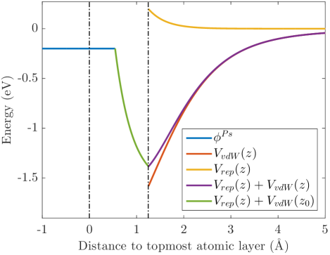
Figure 3: Potential obtained for the Ps model with the values for $C$, $z_{0}$, $\lambda$ and $\phi^{+}$ mentioned in the discussion. For the electronic workfunction, we took $\phi^{-}=4.612~{}\text{eV}$, which gives a Ps workfunction of $\phi^{Ps}=0.2~{}\text{eV}$ and lies in the middle of the range of values for which the model gives an activation energy in good agreement with the experimental result.

The different contributions to the potential are show in figure 3. The Ps state and its energy are obtained by solving the resulting Schrödinger equation

$$-\frac{\psi^{\prime\prime}}{4}+V(z)\psi=E\psi.$$ (18)

IV Computational results

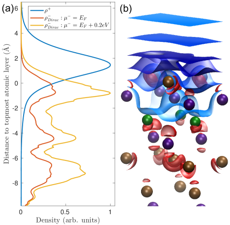
Figure 4: Overlap of the positron SS with the Dirac states. (a) Planar average of the positron (blue) and electron (red/yellow) density associated with the Dirac states below the Fermi-energy for two different values of the chemical potential $\mu^{-}$. (b) Density of the topological surface state and the positron in the same spatial region as panel (a). The progressively lighter blue isosurfaces show the positron density at 80%, 20% and 2% of the maximum value, respectively, and the red isosurfaces show the electronic charge density associated with the electron states on the Dirac cone below the Fermi-level at 10% of the maximum value. The Bi, Te and Se atoms are shown in purple, brown and green colors, respectively.

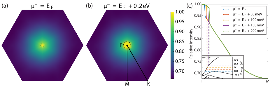
Figure 5: Theoretical momentum densities. (a) LCW map with the chemical potential located at the Fermi-level. (b) LCW map with the chemical potential raised by $0.2\,\text{eV}$. The dashed line denote the location of the Fermi-surface as derived from the electronic bandstructure. (c) High resolution cuts through the LCW map along the $\Gamma$-$M$ direction for different values of the chemical potential. The inset shows the band structure near the Fermi-level $(E_{F}=0.0\,\text{eV})$.

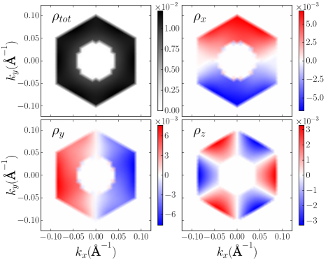
Figure 6: Difference between the LCW maps obtained with different doping levels of the Dirac cone: $\mu^{-}=E_{F}+0.2\,\text{eV}$ and $\mu^{-}=E_{F}$. The top left pane of the figure show the total amplitude of the LCW map. The top right, bottom left and bottom right figures show the magnetization components along the $x$-, $y$- and $z$-axes respectively. We only show the result zoomed in around the $\Gamma$-point as the difference between the LCW maps is exactly zero in the rest of the Brillouin zone. The inner- and othermost edges of the non-zero part in the plots correspond with the dashed lines shown in figures 5(a) and 5(b), respectively. The length of the reciprocal axes is $|\textbf{b}|=1.688\,\text{\AA}^{-1}$ and the amplitudes are given in $\text{ps}^{-1}\text{\AA}^{2}$. (It is readidly seen that the units of the LCW map are in $\text{ps}^{-1}\text{\AA}^{2}$ by realizing that the integral over the LCW map yields the positron’s annihilation rate, or, in the case of the magnetic LCW maps, the difference in annihilation rate between two measurements with opposite spin polarizations for the positron.)

We start our discussion of the computations by showing that the measured Ps activation energy $E_{a}=0.4~{}\text{eV}$ Shastry et al. (2015) is consistent with the theoretical predictions. We take the activation energy to be equal to the groundstate energy predicted by the Ps model discussed in the previous section. For the parameters in the model, we find that the Van der Waals interaction strength evaluates to $C=2.306~{}\text{eV}\cdot\text{\AA}^{3}$ and from the electronic and positronic workfunctions $\phi^{-}=4.904~{}\text{eV}$ and $\phi^{+}=2.392~{}\text{eV}$, we obtain $\phi^{Ps}=0.493~{}\text{eV}$. The values for the background edge position and the characteristic length of the electron density decay in the vacuum region are given by $z_{0}=1.250~{}\text{\AA}$ and $\lambda=0.365~{}\text{\AA}$. Using these values, the model predicts that the Ps forms a delocalized state in the bulk of the material. We note, though, that the experimental value for the electronic workfunction $\phi^{-}=4.5~{}\text{eV}$ is lower than the theoretical one. It is thus sensible to consider the outcome of the model for $\phi^{-}\in[4.5,4.9]~{}\text{eV}$. Over the range $\phi^{-}=4.90~{}\text{eV}$ to $\phi^{-}=4.72~{}\text{eV}$, we find that the groundstate gradually shifts from the bulk to the surface. To determine when we have a surface state, we set the criterion that the Ps density should decay below 1% of its maximum value beyond the first QL block inside the material. In the range $\phi^{-}\in[4.52,4.72]~{}\text{eV}$, the Ps model predicts a surface state with a binding energy of $E_{Ps}=0.40\pm 0.05~{}\text{eV}$, in good agreement with the experimental results.
Next, we investigate the predictions of the 2CDFT calculations to determine whether they support the proposed interpretation of the PAES and AMPS experiments. Our first observation is that the positron in its groundstate indeed resides in the surface’s image potential well rather than the gaps in between the QLs, which also act as strong positron traps. We obtain the binding energy of the positron by taking the difference between the vacuum level and the positron’s chemical potential. The vacuum level is determined in the usual way by the taking the value of the Hartree potential in middle of the vacuum region. We find that the positron SS has a binding energy of $E_{b}=2.69~{}\text{eV}$, in excellent agreement with the measured value. We find that the lifetime evaluates to $\tau=309.25\,\text{ps}$. This value seems reasonable compared with the lifetime of $340-380\,\text{ps}$ measured for positrons trapped at the surface of colloidal PbSe quantum dots Chai et al. (2013). On the other hand, a lifetime of $580\,\text{ps}$ has been determined for positrons trapped at an Al surface Lynn et al. (1984), which can not be reproduced within the LDA approximation Nieminen and Puska (1983). One workaround suggested in literature is to set the enhancement factor to zero for $z>z_{0}$, i.e. assume that the positron will not annihilate in the vacuum region Nieminen et al. (1984). We find, though, that this operation makes the result for the lifetime depend sensitively on the value for the image potential reference plane $z_{0}$. For this reason, as well as the scarcity of experimental data that show this operation is justified, the rest of our calculations have been carried out without modifying the LDA enhancement factor.
Now that the calculations confirmed the existence of the bound positron SS, we turn to the important question of the extent to which this SS overlaps with the Dirac cone electrons. This overlap is of central importance because it determines the annihilation rate of the positron with the electrons occupying the topological states and thus the sensitivity with which positron annihilation spectroscopy can probe the Dirac states. This can be seen from eq. (12), where the partial annihilation rate is determined by the sum over $\lambda_{j}$ where $j$ denotes the states on the cone.
The computed densities of the positron SS, $\rho^{+}$, and the topological Dirac states, $\rho^{-}_{\text{Dirac}}$, are shown in figure 4. The density of the topological states is obtained by summing the one-particle densities for all states on the cone between the Dirac point and a specific value for the electron chemical potential $\mu^{-}$. Although the positron is seen to probe only the topmost atomic layers of the material, it still penetrates the material sufficiently to have a significant overlap with the Dirac states. Moreover, the left panel of figure 4 shows that the overlap with the Dirac states changes sensitively depending on the population of the Dirac states near the Fermi-level. Our calculations of the momentum density, discussed below, further demonstrate that this underlying overlap translates into a clear signal coming from the annihilation of the positron with the Dirac fermions.
A partially filled energy band when it crosses the Fermi energy gives rise to a break in the electron momentum density, which is the basis of the measurement of Fermi surfaces in materials via 2D-ACAR experiments. A standard procedure for enhancing the Fermi surface signal in the spectrum is the Lock-Crisp-West (LCW) map obtained by folding all the higher momentum (Umklapp) contributions into the first Brillouin zone Lock et al. (1973). Figure 5 shows the calculated LCW map together with a cut along $\Gamma-M$ over a range of values of the electron chemical potential, which simulates different doping levels of the Dirac cone. The evolution of the plateau around the $\Gamma$-point clearly indicates the sensitivity of the positron to the Dirac cone states. The relative drop in intensity between $5\%-7\%$ at the Fermi momentum compares favorably with, for example, the 1% drop found for the Nd_2-xCe_xCuO_4-δ high $T_{c}$ superconductor in which 2D-ACAR experiments have been shown previously to be viable in detecting Fermi surface sheets due to Cu-O planes Barbiellini et al. (1995); *Shukla1996.
A topic which has drawn considerable interest in the case of topological insulators, is the spin-momentum locking of the topological states. Measurements using spin-polarised positron beams exploit the fact that a two photon decay is only possible between electrons and positrons with opposite spins Berko and Zuckerman (1964). In recent work, spin-effects in the electronic structure of simple ferromagnets were observed using differences between the doppler broadening of the annihilation radiation (DBAR) measured with positron aligned parallel and anti-parallel to a polarizing magnetic field. Kawasuso et al. (2012). In a similar ACAR experiment, Weber et al. Weber et al. (2015) successfully resolved the spin-dependent Fermi surface of the ferromagnetic Heusler compound Cu₂MnAl. This motivates us to investigate whether spin-polarised positrons can be used to detect the spin-structure of the topological states at the surface. The signal from the Fermi-surface can be extracted from the LCW map by taking the difference between the signal obtained at different doping levels. In figure 6, we show the results obtained by taking the difference between the LCW maps obtained with $\mu^{-}=E_{F}+0.2\,\text{eV}$ and $\mu^{-}=E_{F}$ in the vicinity of the $\Gamma$-point. As expected, we see the plateau due to the extra occupation of the cone in the total amplitude. Our results for the magnetization along the $x$- and $y$-directions, agree well with the results obtained in several studies of various tetradymite TIs Henk et al. (2012); Basak et al. (2011); Lin et al. (2011); Wang and Johnson (2011), which all predict a clockwise rotation of the spin. We see that the $z$-component of the magnetization increases gradually away from the $\Gamma$-point. This out of plane component develops due to the hexagonal warping of the Dirac cone, as pointed out by Fu Fu (2009). We note that the difference in amplitude for the magnetic components is quite pronounced w.r.t. to the Fermi-surface signal. Indeed, we find that the signal from the magnetization about half that of the Fermi-surface signal obtainable with an unpolarized beam. This means that the magnetization signal still constitutes a promising $2\%-4\%$ of the total signal. We note, though, that in real experiments, positron beams are not perfectly polarized, as we have assumed in our calculations. Thus, in experiment, a proper weighting has to be performed which will lead to a smaller signal.

V Conclusion and Outlook

Our study establishes the existence of a positron surface state near the topological insulator Bi₂Te₂Se. The results of our calculations show that this surface state can be exploited as a spectroscopic characterization tool for probing surfaces of topological materials. Since a significant fraction of positrons annihilate with electrons occupying Dirac cone states, 2D-ACAR experiments should be able to measure their momentum distribution with high precision Dugdale et al. (2013), and thus obtain information concerning the nature of the Dirac states which is complementary to that accessed through angle-resolved photoemission, scanning tunnelling and other surface-sensitive spectroscopies without complications of related matrix element effects Bansil and Lindroos (1999); *Campuzano1991; *Nieminen2009. PAES and Doppler broadening of the annihilation radiation Tuomisto and Makkonen (2013) measurements can, in turn, be used to characterize the chemical composition of surfaces. In combination with 2D-ACAR experiments, these positron spectroscopies could be exploited to determine effects of various surface impurities on the topological states, in addition to the role of bulk defects Devidas et al. (2014). Now our study identified a positron surface state, positron spectroscopies can prove valuable for the characterization of nano-structured topological insulators. Indeed, positrons have shown to act as effective self-seeking probes for nano-crystal surfaces without requiring the preparation of single crystal specimens Eijt et al. (2006), whereas the applicability of conventional spectroscopic techniques is limited. Finally, our calculations show that the spin-textures of the Dirac states should be accessible through 2D-ACAR measurements using a spin-polarized positron beam since positrons predominantly annihilate with electrons of the opposite spin Berko and Zuckerman (1964); Kawasuso et al. (2012); Weber et al. (2015).

VI Acknowledgements

I. M. acknowledges discussions with M. Ervasti and A. Harju.
V. C. and R. S. were supported by the FWO-Vlaanderen through Project No. G. 0224.14N. The computational resources and services used in this work were in part provided by the VSC (Flemish Supercomputer Center) and the HPC infrastructure of the University of Antwerp (CalcUA), both funded by the Hercules Foundation and the Flemish Government (EWI Department). I. M. acknowledges financial support from the Academy of Finland (projects 285809 and 293932). The work at Northeastern University was supported by the US Department of Energy (DOE), Office of Science, Basic Energy Sciences grant number DE-FG02-07ER46352, and benefited from Northeastern University’s Advanced Scientific Computation Center (ASCC) and the NERSC supercomputing center through DOE grant number DE-AC02-05CH11231. K. S. and A. W. acknowledge financial support from the National Science Foundation through grants DMR-MRI-1338130 and DMR-1508719. D. H. received financial support of the National Science Foundation (grant ECCS-1402738). J. S. M. was supported by the STC Center for Integrated Quantum Materials under NSF grant DMR-1231319, NSF DMR-1207469 and ONR N00014-13-1-0301. B. A. A. also acknowledges support from the LabEx ENS-ICFP: ANR-10-LABX-0010/ANR-10-IDEX-0001-02 PSL.

VII References

Appendix A Detailed derivation spin-resolved momentum density

In this appendix, we give a detailed derivation of the momentum density formulas given in the main manuscript. We start from the general expression given in ref. Ryzhikh and Mitroy, 1999, which defines the rate to start with the ground-state with $N$ electron and a single positron $\Psi$ and end up in the final state $\Phi$, with $N-1$ electrons and two photons with total momentum p:

$$\begin{split}\Lambda_{\nu}(\textbf{p})&=4\pi r_{e}^{2}c\displaystyle\sum_{i=1}^{N}\sum_{s_{i},s_{p}}\bigg{|}\int d\tau\int d\textbf{r}_{i}\int d\textbf{r}_{p}\,\Phi^{*}_{\nu}(\textbf{x}_{1},\dots,\textbf{x}_{i-1},\textbf{x}_{i+1},\dots,\textbf{x}_{N})e^{-i\textbf{p}\cdot\textbf{r}_{p}}\\ &\quad\times\hat{S}^{s}_{i}\,\delta(\textbf{r}_{i}-\textbf{r}_{p})\,\Psi(\textbf{x}_{1},\dots,\textbf{x}_{N};\textbf{x}_{p})\bigg{|}^{2}.\end{split}$$ (19)

To keep notation in check, we define $\textbf{x}_{i}=\{\textbf{r}_{i},s_{i}\}$ to denote the particle position and spin, and $d\tau=\prod_{j=1,j\neq i}^{N}d\textbf{x}_{j}$ to represent integration over all the non-annihilating electron coordinates, thus including a sum over the possible spin directions of the particle. The contraint that only electron-positron pairs in a singlet state contribute to the 2$\gamma$ annihilation is taken into account through the operator $\hat{S}^{s}_{i}=1-\hat{S}^{2}/2$, with $\hat{S}_{i}^{2}$ the total spin operator of electron $i$ and the positron. As we will show further on, this operator projects the electron-positron pair on the singlet states of the respective pairs.
Thanks to the anti-symmetry of the wavefunction, we can swap the electron indices around such that the annihilating electron always has the label $N$. We make use of the delta function to get perform the integration over the positron coordinate to get:

$$\Lambda_{\nu}(\textbf{p})=4\pi r_{e}^{2}c\,N\displaystyle\sum_{s_{N},s_{p}}\left|\int d\tau\int d\textbf{r}_{N}\,\Phi^{*}_{\nu}(\textbf{x}_{1},\dots,\textbf{x}_{N-1})\,e^{-i\textbf{p}\cdot\textbf{r}_{N}}\,\hat{S}^{s}_{N}\,\Psi(\textbf{r}_{1},s_{1},\dots,\textbf{r}_{N},s_{N};\textbf{r}_{N},s_{p})\right|^{2}.$$ (20)

If we are not concerned with the precise final state $\Phi^{*}_{\nu}$ we end up with, we can define the 2$\gamma$ transition rate $\rho(\textbf{p})=\sum_{\nu}\Lambda_{\nu}(\textbf{p})$ from $\Psi$ to some final state with a pair of photons of total momentum p. The completeness relation:

$$\sum_{\nu}\Phi^{*}_{\nu}(\textbf{x}_{1},\dots,\textbf{x}_{N-1})\Phi_{\nu}(\textbf{x}^{\prime}_{1},\dots,\textbf{x}^{\prime}_{N-1})=\delta(\textbf{x}_{1}-\textbf{x}^{\prime}_{1})\dots\delta(\textbf{x}_{N-1}-\textbf{x}^{\prime}_{N-1}),$$ (21)

then allows us to write:

$$\rho(\textbf{p})=4\pi r_{e}^{2}cN\displaystyle\sum_{s_{e},s_{p}}\int d\textbf{x}_{1}\dots\int d\textbf{x}_{N-1}\left|\int d\textbf{r}_{N}\,e^{i\textbf{p}\cdot\textbf{x}_{N}}\,\hat{S}^{s}_{N}\,\Psi(\textbf{x}_{1},\dots,\textbf{r}_{N},s_{N};\textbf{r}_{N},s_{p})\right|^{2}.$$ (22)

We now recognize the electron-positron two-body reduced density matrix, defined as Makkonen et al. (2005); Zubiaga et al. (2016):

$$\begin{split}\Gamma^{ep}(\textbf{r}_{e},s_{e},\textbf{r}_{p},s_{p};\textbf{r}^{\prime}_{e},s_{e}^{\prime},\textbf{r}^{\prime}_{p},s_{p}^{\prime})&=N\int d\textbf{x}_{1}\dots\int d\textbf{x}_{N-1}\,\Psi^{*}(\textbf{x}_{1},\dots,\textbf{x}_{N-1},\textbf{r}_{e},s_{e};\textbf{r}_{p},s_{p})\\ &\quad\times\Psi(\textbf{x}_{1},\dots,\textbf{x}_{N-1},\textbf{r}^{\prime}_{e},s^{\prime}_{e};\textbf{r}^{\prime}_{p},s^{\prime}_{p}).\end{split}$$ (23)

It is convenient to introduce the natural geminals, also called pairing-wavefunctions, which diagonalize the above density matrix:

$$\Gamma^{ep}(\textbf{r}_{e},s_{e},\textbf{r}_{p},s_{p};\textbf{r}^{\prime}_{e},s_{e}^{\prime},\textbf{r}^{\prime}_{p},s_{p}^{\prime})=\displaystyle\sum_{j}g_{j}\,\alpha^{*}_{j}(\textbf{r}_{e},s_{e};\textbf{r}_{p},s_{p})\,\alpha_{j}(\textbf{r}^{\prime}_{e},s_{e}^{\prime};\textbf{r}^{\prime}_{p},s_{p}^{\prime}).$$ (24)

We thus arrive at the general expression for the 2$\gamma$ momentum density:

$$\rho(\textbf{p})=4\pi r_{e}^{2}c\displaystyle\sum_{j}g_{j}\sum_{s_{e},s_{p}}\left|\int d\textbf{r}\,e^{-i\textbf{p}\cdot\textbf{r}}\,\hat{S}^{s}\,\alpha_{j}(\textbf{r},s_{e};\textbf{r},s_{p})\right|^{2},$$ (25)

where we dropped the now unnecessary label on the singlet operator.
Let us now examine the effect of the singlet projection operator. We have:

$$\begin{split}\hat{S}^{s}&=1-\frac{\hat{S}^{2}}{2}\\ &=1-\frac{1}{2}\left(\hat{S}^{2}_{s_{e}}+\hat{S}^{2}_{s_{p}}+2\,\hat{\textbf{S}}_{s_{e}}\cdot\hat{\textbf{S}}_{s_{p}}\right)\\ &=1-\frac{1}{2}\left(\hat{S}^{2}_{s_{e}}+\hat{S}^{2}_{s_{p}}+2\,\left[\hat{S}_{s_{e},x}\hat{S}_{s_{p},x}+\hat{S}_{s_{e},y}\hat{S}_{s_{p},y}+\hat{S}_{s_{e},z}\hat{S}_{s_{p},z}\right]\right)\end{split}$$ (26)

If we make use of:

$$\begin{split}\hat{S}^{2}_{s_{e}}|{s_{e},s_{p}}\rangle&=\hat{S}^{2}_{s_{p}}|{s_{e},s_{p}}\rangle=\frac{3}{4}|{s_{e},s_{p}}\rangle\\ \hat{S}_{s_{e},x}\hat{S}_{s_{p},x}|{s_{e},s_{p}}\rangle&=|s_{e}s_{p}||{-s_{e},-s_{p}}\rangle=\frac{1}{4}|{-s_{e},-s_{p}}\rangle\\ \hat{S}_{s_{e},y}\hat{S}_{s_{p},y}|{s_{e},s_{p}}\rangle&=-s_{e}s_{p}|{-s_{e},-s_{p}}\rangle\\ \hat{S}_{s_{e},z}\hat{S}_{s_{p},z}|{s_{e},s_{p}}\rangle&=s_{e}s_{p}|{s_{e},s_{p}}\rangle,\end{split}$$ (27)

then we find:

$$\hat{S}^{s}|{s_{e},s_{p}}\rangle=\left(\frac{1}{4}-s_{e}s_{p}\right)\left(|{s_{e},s_{p}}\rangle-|{-s_{e},-s_{p}}\rangle\right).$$ (28)

It is obvious that this gives zero if the electron and positron spins have the same value and the prefactor becomes $1/2$ when they are anti-parallel. Note that this operator thus indeed projects on the singlet states $\pm(|{\uparrow\downarrow}\rangle-|{\downarrow\uparrow}\rangle)$.
After performing the sum over all electron and positron spins, we find for the momentum density expression:

$$\begin{split}\rho(\textbf{p})&=4\pi r_{e}^{2}c\displaystyle\sum_{j}g_{j}\left|\int d\textbf{r}e^{-i\textbf{p}\cdot\textbf{r}}\frac{1}{\sqrt{2}}\left(\alpha_{j}(\textbf{r},\uparrow;\textbf{r},\downarrow)-\alpha_{j}(\textbf{r},\downarrow;\textbf{r},\uparrow)\right)\right|^{2}\\ &=2\pi r_{e}^{2}c\sum_{j}g_{j}\int d\textbf{r}\int d\textbf{r}^{\prime}e^{-i\textbf{p}\cdot(\textbf{r}-\textbf{r}^{\prime})}\Big{[}\alpha_{j}(\textbf{r},\uparrow;\textbf{r},\downarrow)\alpha^{*}_{j}(\textbf{r}^{\prime},\uparrow;\textbf{r}^{\prime},\downarrow)+\alpha_{j}(\textbf{r},\downarrow;\textbf{r},\uparrow)\alpha^{*}_{j}(\textbf{r}^{\prime},\downarrow;\textbf{r}^{\prime},\uparrow)\\ &\quad-\alpha_{j}(\textbf{r},\downarrow;\textbf{r},\uparrow)\alpha^{*}_{j}(\textbf{r}^{\prime},\uparrow;\textbf{r}^{\prime},\downarrow)-\alpha_{j}(\textbf{r},\uparrow;\textbf{r},\downarrow)\alpha^{*}_{j}(\textbf{r}^{\prime},\downarrow;\textbf{r}^{\prime},\uparrow)\Big{]}.\\ \end{split}$$ (29)

In the rest of the derivation, it is more convenient to work with a spinor representation for the geminals, which we define as:

$$\alpha_{j}(\textbf{r}_{e};\textbf{r}_{p})=\begin{pmatrix}\alpha_{j}(\textbf{r}_{e},\uparrow;\textbf{r}_{p},\uparrow)\\ \alpha_{j}(\textbf{r}_{e},\uparrow;\textbf{r}_{p},\downarrow)\\ \alpha_{j}(\textbf{r}_{e},\downarrow;\textbf{r}_{p},\uparrow)\\ \alpha_{j}(\textbf{r}_{e},\downarrow;\textbf{r}_{p},\downarrow)\end{pmatrix}.$$ (30)

Equation (25) then becomes:

$$\begin{split}\rho(\textbf{p})&=4\pi r_{e}^{2}c\sum_{j}g_{j}\bigg{|}\int d\textbf{r}\,e^{-i\textbf{p}\cdot\textbf{r}}\hat{S}^{s}\alpha_{j}(\textbf{r};\textbf{r})\bigg{|}^{2}\\ &=4\pi r_{e}^{2}c\sum_{j}g_{j}\int d\textbf{r}\int d\textbf{r}^{\prime}\,e^{-i\textbf{p}\cdot(\textbf{r}-\textbf{r}^{\prime})}\left[\hat{S}^{s}\alpha_{j}^{\dagger}(\textbf{r}^{\prime};\textbf{r}^{\prime})\right]\left[\hat{S}^{s}\alpha_{j}(\textbf{r}^{\prime};\textbf{r}^{\prime})\right].\end{split}$$ (31)

Indeed, making use of:

$$\hat{S}^{s}\alpha_{j}(\textbf{r}_{e};\textbf{r}_{p})=\frac{1}{2}\begin{pmatrix}0\\ \alpha_{j}(\textbf{r}_{e},\uparrow;\textbf{r}_{p},\downarrow)-\alpha_{j}(\textbf{r}_{e},\downarrow;\textbf{r}_{p},\uparrow)\\ \alpha_{j}(\textbf{r}_{e},\downarrow;\textbf{r}_{p},\uparrow)-\alpha_{j}(\textbf{r}_{e},\uparrow;\textbf{r}_{p},\downarrow)\\ 0\end{pmatrix},$$ (32)

it is straightforward to check that one obtains the same result asin equation (29).
Next, if we assume that the geminals are collinear in the positron spin, we can write:

$$\alpha_{j}(\textbf{r}_{e};\textbf{r}_{p})=\begin{pmatrix}\alpha_{j}(\textbf{r}_{e},\uparrow;\textbf{r}_{p})\\ \alpha_{j}(\textbf{r}_{e},\downarrow;\textbf{r}_{p})\\ \end{pmatrix}\otimes\chi_{p},$$ (33)

where $\otimes$ denotes a direct product, the remaining arrow indicates the electron spin, and $\chi_{p}$ is the (position-independent) spinor for the positron. For a positron fully polarized along the positive and negative $z$-axis, respectively, we have the single particle spinors:

$$\chi_{p}^{z^{+}}=\begin{pmatrix}1\\ 0\end{pmatrix}\quad\text{and}\quad\chi_{p}^{z^{-}}=\begin{pmatrix}0\\ 1\end{pmatrix}.$$ (34)

For the geminal spinor this gives:

$$\alpha^{z^{+}}_{j}(\textbf{r}_{e};\textbf{r}_{p})=\begin{pmatrix}\alpha_{j}(\textbf{r}_{e},\uparrow;\textbf{r}_{p},\uparrow)\\ 0\\ \alpha_{j}(\textbf{r}_{e},\downarrow;\textbf{r}_{p},\uparrow)\\ 0\end{pmatrix},\quad\text{and}\quad\alpha^{z^{-}}_{j}(\textbf{r}_{e};\textbf{r}_{p})=\begin{pmatrix}0\\ \alpha_{j}(\textbf{r}_{e},\uparrow;\textbf{r}_{p},\downarrow)\\ 0\\ \alpha_{j}(\textbf{r}_{e},\downarrow;\textbf{r}_{p},\downarrow)\end{pmatrix}.$$ (35)

and after applying the singlet operator to them:

$$\hat{S}^{s}\alpha^{z^{+}}_{j}(\textbf{r}_{e};\textbf{r}_{p})=\frac{1}{2}\begin{pmatrix}0\\ 0\\ \alpha_{j}(\textbf{r}_{e},\downarrow;\textbf{r}_{p},\uparrow)\\ 0\end{pmatrix},\quad\text{and}\quad\hat{S}^{s}\alpha^{z^{-}}_{j}(\textbf{r}_{e};\textbf{r}_{p})=\frac{1}{2}\begin{pmatrix}0\\ \alpha_{j}(\textbf{r}_{e},\uparrow;\textbf{r}_{p},\downarrow)\\ 0\\ 0\\ \end{pmatrix}.$$ (36)

From (31) we obtain:

$$\begin{split}\rho_{z^{+}}(\textbf{p})&=2\pi r_{e}^{2}c\sum_{j}g_{j}\int d\textbf{r}\int d\textbf{r}^{\prime}\,e^{-i\textbf{p}\cdot(\textbf{r}-\textbf{r}^{\prime})}\alpha_{j}(\textbf{r},\downarrow;\textbf{r},\uparrow)\alpha^{*}_{j}(\textbf{r}^{\prime},\downarrow;\textbf{r}^{\prime},\uparrow)\\ \rho_{z^{-}}(\textbf{p})&=2\pi r_{e}^{2}c\sum_{j}g_{j}\int d\textbf{r}\int d\textbf{r}^{\prime}\,e^{-i\textbf{p}\cdot(\textbf{r}-\textbf{r}^{\prime})}\alpha_{j}(\textbf{r},\uparrow;\textbf{r},\downarrow)\alpha^{*}_{j}(\textbf{r}^{\prime},\uparrow;\textbf{r}^{\prime},\downarrow).\end{split}$$ (37)

The magnetization is obtained as the difference between these two spectra and gives:

$$\rho_{z}(\textbf{p})=\rho_{z^{-}}(\textbf{p})-\rho_{z^{+}}(\textbf{p})=2\pi r_{e}^{2}c\displaystyle\sum_{j}g_{j}\left[\bigg{|}\int d\textbf{r}e^{-i\textbf{p}\cdot\textbf{r}}\alpha_{j}(\textbf{r},\uparrow;\textbf{r},\downarrow)\bigg{|}^{2}-\bigg{|}\int d\textbf{r}e^{-i\textbf{p}\cdot\textbf{r}}\alpha_{j}(\textbf{r},\downarrow;\textbf{r},\uparrow)\bigg{|}^{2}\right]$$ (38)

A positron polarized along the $x$-axis is represented by the single particle spinors:

$$\chi_{p}^{x^{+}}=\frac{1}{\sqrt{2}}\begin{pmatrix}1\\ 1\end{pmatrix}\quad\text{and}\quad\chi_{p}^{x^{-}}=\frac{1}{\sqrt{2}}\begin{pmatrix}1\\ -1\end{pmatrix}.$$ (39)

Thus we get:

$$\alpha^{x^{+}}_{j}(\textbf{r};\textbf{r})=\frac{1}{\sqrt{2}}\begin{pmatrix}\alpha_{j}(\textbf{r},\uparrow;\textbf{r},\uparrow)\\ \alpha_{j}(\textbf{r},\uparrow;\textbf{r},\downarrow)\\ \alpha_{j}(\textbf{r},\downarrow;\textbf{r},\uparrow)\\ \alpha_{j}(\textbf{r},\downarrow;\textbf{r},\downarrow)\end{pmatrix},\quad\alpha^{x^{-}}_{j}(\textbf{r};\textbf{r})=\frac{1}{\sqrt{2}}\begin{pmatrix}\alpha_{j}(\textbf{r},\uparrow;\textbf{r},\uparrow)\\ -\alpha_{j}(\textbf{r},\uparrow;\textbf{r},\downarrow)\\ \alpha_{j}(\textbf{r},\downarrow;\textbf{r},\uparrow)\\ -\alpha_{j}(\textbf{r},\downarrow;\textbf{r},\downarrow)\end{pmatrix},$$ (40)

and:

$$\hat{S}^{s}\alpha^{x^{+}}_{j}(\textbf{r};\textbf{r})=\frac{1}{2\sqrt{2}}\begin{pmatrix}0\\ \alpha_{j}(\textbf{r},\uparrow;\textbf{r},\downarrow)-\alpha_{j}(\textbf{r},\downarrow;\textbf{r},\uparrow)\\ \alpha_{j}(\textbf{r},\downarrow;\textbf{r},\uparrow)-\alpha_{j}(\textbf{r},\uparrow;\textbf{r},\downarrow)\\ 0\\ \end{pmatrix},\quad\hat{S}^{s}\alpha^{x^{-}}_{j}(\textbf{r};\textbf{r})=\frac{1}{2\sqrt{2}}\begin{pmatrix}0\\ -\alpha_{j}(\textbf{r},\uparrow;\textbf{r},\downarrow)-\alpha_{j}(\textbf{r},\downarrow;\textbf{r},\uparrow)\\ \alpha_{j}(\textbf{r},\downarrow;\textbf{r},\uparrow)+\alpha_{j}(\textbf{r},\uparrow;\textbf{r},\downarrow)\\ 0\\ \end{pmatrix},$$ (41)

which result in the momentum densities:

$$\begin{split}\rho_{x^{+}}(\textbf{p})&=2\pi r_{e}^{2}c\sum_{j}g_{j}\int d\textbf{r}\int d\textbf{r}^{\prime}e^{-i\textbf{p}\cdot(\textbf{r}-\textbf{r}^{\prime})}\frac{1}{2}\Big{[}\alpha_{j}(\textbf{r},\uparrow;\textbf{r},\downarrow)\alpha^{*}_{j}(\textbf{r}^{\prime},\uparrow;\textbf{r}^{\prime},\downarrow)+\alpha_{j}(\textbf{r},\downarrow;\textbf{r},\uparrow)\alpha^{*}_{j}(\textbf{r}^{\prime},\downarrow;\textbf{r}^{\prime},\uparrow)\\ &\quad-\alpha_{j}(\textbf{r},\downarrow;\textbf{r},\uparrow)\alpha^{*}_{j}(\textbf{r}^{\prime},\uparrow;\textbf{r}^{\prime},\downarrow)-\alpha_{j}(\textbf{r},\uparrow;\textbf{r},\downarrow)\alpha^{*}_{j}(\textbf{r}^{\prime},\downarrow;\textbf{r}^{\prime},\uparrow)\Big{]}.\\ \rho_{x^{-}}(\textbf{p})&=2\pi r_{e}^{2}c\sum_{j}g_{j}\int d\textbf{r}\int d\textbf{r}^{\prime}e^{-i\textbf{p}\cdot(\textbf{r}-\textbf{r}^{\prime})}\frac{1}{2}\Big{[}\alpha_{j}(\textbf{r},\uparrow;\textbf{r},\downarrow)\alpha^{*}_{j}(\textbf{r}^{\prime},\uparrow;\textbf{r}^{\prime},\downarrow)+\alpha_{j}(\textbf{r},\downarrow;\textbf{r},\uparrow)\alpha^{*}_{j}(\textbf{r}^{\prime},\downarrow;\textbf{r}^{\prime},\uparrow)\\ &\quad+\alpha_{j}(\textbf{r},\downarrow;\textbf{r},\uparrow)\alpha^{*}_{j}(\textbf{r}^{\prime},\uparrow;\textbf{r}^{\prime},\downarrow)+\alpha_{j}(\textbf{r},\uparrow;\textbf{r},\downarrow)\alpha^{*}_{j}(\textbf{r}^{\prime},\downarrow;\textbf{r}^{\prime},\uparrow)\Big{]}.\\ \end{split}$$ (42)

So the magnetization in this case is:

$$\begin{split}\rho_{x}(\textbf{p})=\rho_{x^{-}}(\textbf{p})-\rho_{x^{+}}(\textbf{p})&=2\pi r_{e}^{2}c\sum_{j}g_{j}\int d\textbf{r}\int d\textbf{r}^{\prime}e^{-i\textbf{p}\cdot(\textbf{r}-\textbf{r}^{\prime})}\\ &\quad\times\Big{[}\alpha_{j}(\textbf{r},\downarrow;\textbf{r},\uparrow)\alpha^{*}_{j}(\textbf{r}^{\prime},\uparrow;\textbf{r}^{\prime},\downarrow)+\alpha_{j}(\textbf{r},\uparrow;\textbf{r},\downarrow)\alpha^{*}_{j}(\textbf{r}^{\prime},\downarrow;\textbf{r}^{\prime},\uparrow)\Big{]}\end{split}$$ (43)

Finally, a positron polarized along the $y$-axis is represented by the single particle spinors:

$$\chi_{p}^{y^{+}}=\frac{1}{\sqrt{2}}\begin{pmatrix}1\\ i\end{pmatrix}\quad\text{and}\quad\chi_{p}^{y^{-}}=\frac{1}{\sqrt{2}}\begin{pmatrix}1\\ -i\end{pmatrix}.$$ (44)

The geminal spinors become:

$$\alpha^{y^{+}}_{j}(\textbf{r};\textbf{r})=\frac{1}{\sqrt{2}}\begin{pmatrix}\alpha_{j}(\textbf{r},\uparrow;\textbf{r},\uparrow)\\ i\alpha_{j}(\textbf{r},\uparrow;\textbf{r},\downarrow)\\ \alpha_{j}(\textbf{r},\downarrow;\textbf{r},\uparrow)\\ i\alpha_{j}(\textbf{r},\downarrow;\textbf{r},\downarrow)\end{pmatrix},\quad\alpha^{y^{-}}_{j}(\textbf{r};\textbf{r})=\frac{1}{\sqrt{2}}\begin{pmatrix}\alpha_{j}(\textbf{r},\uparrow;\textbf{r},\uparrow)\\ -i\alpha_{j}(\textbf{r},\uparrow;\textbf{r},\downarrow)\\ \alpha_{j}(\textbf{r},\downarrow;\textbf{r},\uparrow)\\ -i\alpha_{j}(\textbf{r},\downarrow;\textbf{r},\downarrow)\end{pmatrix},$$ (45)

$$\hat{S}^{s}\alpha^{y^{+}}_{j}(\textbf{r};\textbf{r})=\frac{1}{2\sqrt{2}}\begin{pmatrix}0\\ i\alpha_{j}(\textbf{r},\uparrow;\textbf{r},\downarrow)-\alpha_{j}(\textbf{r},\downarrow;\textbf{r},\uparrow)\\ \alpha_{j}(\textbf{r},\downarrow;\textbf{r},\uparrow)-i\alpha_{j}(\textbf{r},\uparrow;\textbf{r},\downarrow)\\ 0\\ \end{pmatrix},\quad\hat{S}^{s}\alpha^{y^{-}}_{j}(\textbf{r};\textbf{r})=\frac{1}{2\sqrt{2}}\begin{pmatrix}0\\ -i\alpha_{j}(\textbf{r},\uparrow;\textbf{r},\downarrow)-\alpha_{j}(\textbf{r},\downarrow;\textbf{r},\uparrow)\\ \alpha_{j}(\textbf{r},\downarrow;\textbf{r},\uparrow)+i\alpha_{j}(\textbf{r},\downarrow;\textbf{r},\uparrow)\\ 0\\ \end{pmatrix},$$ (46)

from which we find:

$$\begin{split}\rho_{y^{+}}(\textbf{p})&=2\pi r_{e}^{2}c\sum_{j}g_{j}\int d\textbf{r}\int d\textbf{r}^{\prime}e^{-i\textbf{p}\cdot(\textbf{r}-\textbf{r}^{\prime})}\frac{1}{2}\Big{[}\alpha_{j}(\textbf{r},\uparrow;\textbf{r},\downarrow)\alpha^{*}_{j}(\textbf{r}^{\prime},\uparrow;\textbf{r}^{\prime},\downarrow)+\alpha_{j}(\textbf{r},\downarrow;\textbf{r},\uparrow)\alpha^{*}_{j}(\textbf{r}^{\prime},\downarrow;\textbf{r}^{\prime},\uparrow)\\ &\quad+i\alpha_{j}(\textbf{r},\downarrow;\textbf{r},\uparrow)\alpha^{*}_{j}(\textbf{r}^{\prime},\uparrow;\textbf{r}^{\prime},\downarrow)-i\alpha_{j}(\textbf{r},\uparrow;\textbf{r},\downarrow)\alpha^{*}_{j}(\textbf{r}^{\prime},\downarrow;\textbf{r}^{\prime},\uparrow)\Big{]}.\\ \rho_{y^{-}}(\textbf{p})&=2\pi r_{e}^{2}c\sum_{j}g_{j}\int d\textbf{r}\int d\textbf{r}^{\prime}e^{-i\textbf{p}\cdot(\textbf{r}-\textbf{r}^{\prime})}\frac{1}{2}\Big{[}\alpha_{j}(\textbf{r},\uparrow;\textbf{r},\downarrow)\alpha^{*}_{j}(\textbf{r}^{\prime},\uparrow;\textbf{r}^{\prime},\downarrow)+\alpha_{j}(\textbf{r},\downarrow;\textbf{r},\uparrow)\alpha^{*}_{j}(\textbf{r}^{\prime},\downarrow;\textbf{r}^{\prime},\uparrow)\\ &\quad-i\alpha_{j}(\textbf{r},\downarrow;\textbf{r},\uparrow)\alpha^{*}_{j}(\textbf{r}^{\prime},\uparrow;\textbf{r}^{\prime},\downarrow)+i\alpha_{j}(\textbf{r},\uparrow;\textbf{r},\downarrow)\alpha^{*}_{j}(\textbf{r}^{\prime},\downarrow;\textbf{r}^{\prime},\uparrow)\Big{]}.\\ \end{split}$$ (47)

This gives the final component of the magnetization:

$$\begin{split}\rho_{y}(\textbf{p})=\rho_{y^{-}}(\textbf{p})-\rho_{y^{+}}(\textbf{p})&=2i\pi r_{e}^{2}c\sum_{j}g_{j}\int d\textbf{r}\int d\textbf{r}^{\prime}e^{-i\textbf{p}\cdot(\textbf{r}-\textbf{r}^{\prime})}\\ &\quad\times\Big{[}\alpha_{j}(\textbf{r}^{\prime},\uparrow;\textbf{r}^{\prime},\downarrow)\alpha^{*}_{j}(\textbf{r},\downarrow;\textbf{r},\uparrow)-\alpha_{j}(\textbf{r}^{\prime},\downarrow;\textbf{r}^{\prime},\uparrow)\alpha^{*}_{j}(\textbf{r},\uparrow;\textbf{r},\downarrow)\Big{]}.\end{split}$$ (48)

If we introduce the notation:

$$A_{j,s_{e},s_{p}}(\textbf{p})=\int d\textbf{r}\,e^{-i\textbf{p}\cdot\textbf{r}}\alpha_{j}(\textbf{r},s_{e};\textbf{r},s_{p})$$ (49)

and the matrix:

$$\Gamma_{j}(\textbf{p})=\begin{pmatrix}|A_{j,\uparrow\downarrow}(\textbf{p})|^{2}&A_{j,\uparrow\downarrow}(\textbf{p})A_{j,\downarrow\uparrow}^{*}(\textbf{p})\\ A_{j,\downarrow\uparrow}(\textbf{p})A_{j,\uparrow\downarrow}^{*}(\textbf{p})&|A_{j,\downarrow\uparrow}(\textbf{p})|^{2}\end{pmatrix},$$ (50)

then the above results can be written as:

$$\rho_{i}(\textbf{p})=2\pi r_{e}^{2}c\displaystyle\sum_{j}g_{j}\text{Tr}\left[\sigma_{i}\Gamma_{j}(\textbf{p})\right],$$ (51)

where $i=\{x,y,z\}$ and $\sigma_{i}$ are the Pauli matrices.
Let us now derive the momentum density as measured in experiments with unpolarized positron beams. In this case, there is a statistical uncertainty on the direction of the positron spin. We can assume that the 50% of the positrons are in the up state and 50% in the down state, w.r.t. whatever direction of the quantization axis. This means we measure:

$$\rho_{\text{tot}}(\textbf{p})=\frac{1}{2}(\rho_{z^{+}}(\textbf{p})+\rho_{z^{-}}(\textbf{p}))=\pi r_{e}^{2}c\displaystyle\sum_{j}g_{j}\text{Tr}\left[\Gamma_{j}(\textbf{p})\right],$$ (52)

which results in the correct prefactor found in literature.

References

- Hasan and Kane (2010) M. Z. Hasan and C. L. Kane, Rev. Mod. Phys. 82, 3045 (2010).
- Bansil et al. (2016) A. Bansil, H. Lin, and T. Das, Rev. Mod. Phys. 88, 021004 (2016).
- Moore (2010) J. E. Moore, Nature 464, 194 (2010).
- Mellnik et al. (2014) A. R. Mellnik, J. S. Lee, A. Richardella, J. L. Grab, P. J. Mintun, M. H. Fischer, A. Vaezi, A. Manchon, E.-A. Kim, N. Samarth, and D. C. Ralph, Nature 511, 449 (2014).
- Mourik et al. (2012) V. Mourik, K. Zuo, S. M. Frolov, S. R. Plissard, E. P. A. M. Bakkers, and L. P. Kouwenhoven, Science 336, 1003 (2012).
- Hsieh et al. (2008) D. Hsieh, D. Qian, L. Wray, Y. Xia, Y. S. Hor, R. J. Cava, and M. Z. Hasan, Nature 452, 970 (2008).
- Hsieh et al. (2009) D. Hsieh, Y. Xia, D. Qian, L. Wray, J. H. Dil, F. Meier, J. Osterwalder, L. Patthey, J. G. Checkelsky, N. P. Ong, A. V. Fedorov, H. Lin, A. Bansil, D. Grauer, Y. S. Hor, R. J. Cava, and M. Z. Hasan, Nature 460, 1101 (2009).
- Roushan et al. (2009) P. Roushan, J. Seo, C. V. Parker, Y. S. Hor, D. Hsieh, D. Qian, A. Richardella, M. Z. Hasan, R. J. Cava, and A. Yazdani, Nature 460, 1106 (2009).
- Xia et al. (2009) Y. Xia, D. Qian, D. Hsieh, L. Wray, A. Pal, H. Lin, A. Bansil, D. Grauer, Y. S. Hor, R. J. Cava, and M. Z. Hasan, Nat. Phys. 5, 398 (2009).
- Berko and Zuckerman (1964) S. Berko and J. Zuckerman, Phys. Rev. Lett. 13, 339 (1964).
- Shastry et al. (2015) K. Shastry, A. H. Weiss, B. Barbiellini, B. A. Assaf, Z. H. Lim, P. V. Joglekar, and D. Heiman, J. Phys.: Conf. Ser. 618, 012006 (2015).
- Assaf et al. (2013) B. A. Assaf, T. Cardinal, P. Wei, F. Katmis, J. S. Moodera, and D. Heiman, Appl. Phys. Lett. 102, 012102 (2013).
- Zhang et al. (2012) D. Zhang, A. Richardella, D. W. Rench, S.-Y. Xu, A. Kandala, T. C. Flanagan, H. Beidenkopf, A. L. Yeats, B. B. Buckley, P. V. Klimov, D. D. Awschalom, A. Yazdani, P. Schiffer, M. Z. Hasan, and N. Samarth, Phys. Rev. B 86, 205127 (2012).
- Weiss et al. (1988) A. Weiss, R. Mayer, M. Jibaly, C. Lei, D. Mehl, and K. G. Lynn, Phys. Rev. Lett. 61, 2245 (1988).
- Mukherjee et al. (2010) S. Mukherjee, M. P. Nadesalingam, P. Guagliardo, A. D. Sergeant, B. Barbiellini, J. F. Williams, N. G. Fazleev, and A. H. Weiss, Phys. Rev. Lett. 104, 247403 (2010).
- Chu et al. (1981) S. Chu, A. P. Mills, and C. A. Murray, Phys. Rev. B 23, 2060 (1981).
- Chakraborty and Siegel (1983) B. Chakraborty and R. W. Siegel, Phys. Rev. B 27, 4535 (1983).
- Boronski and Nieminen (1986) E. Boronski and R. M. Nieminen, Phys. Rev. B 34, 3820 (1986).
- Blöchl (1994) P. E. Blöchl, Phys. Rev. B 50, 17953 (1994).
- Kresse and Furthmüller (1996a) G. Kresse and J. Furthmüller, Comput. Mater. Sci. 6, 15 (1996a).
- Kresse and Furthmüller (1996b) G. Kresse and J. Furthmüller, Phys. Rev. B 54, 11169 (1996b).
- Kresse and Joubert (1999) G. Kresse and D. Joubert, Phys. Rev. B 59, 1758 (1999).
- Perdew et al. (1996) J. P. Perdew, K. Burke, and M. Ernzerhof, Phys. Rev. Lett 77, 3865 (1996).
- Note (1) The distance between the QL blocks is severely overestimated when using the PBE functional. As positrons are strongly repelled by the ions, the separation between the QL strongly influences the value of the positron workfunction and in order to obtain reliable results, we deem it appropriate to work with the experimental lattice parameters instead. The lattice parameters only slightly affect the electronic structure as the results of our bandstructure calculations agree very well with the previously reported first-principles results Dai et al. (2012); Wang and Johnson (2011); Chang et al. (2011); Lin et al. (2011) and those of ARPES measurements Neupane et al. (2012); Arakane et al. (2012).
- Lang and Kohn (1973) N. D. Lang and W. Kohn, Phys. Rev. B 7, 3541 (1973).
- Nieminen and Puska (1983) R. M. Nieminen and M. J. Puska, Phys. Rev. Lett. 50, 281 (1983).
- Note (2) We are updating the standard corrugated mirror model for the potential at the surface Nieminen and Puska (1983); Fazleev et al. (1995, 2004) where GGA corrections Barbiellini and Kuriplach (2015) are traditionally not included.
- Makkonen et al. (2006) I. Makkonen, M. Hakala, and M. J. Puska, Phys. Rev. B 73, 035103 (2006).
- Torsti et al. (2003) T. Torsti, M. Heiskanen, M. J. Puska, and R. M. Nieminen, Int. J. Quantum Chem. 91, 171 (2003).
- Torsti et al. (2006) T. Torsti, T. Eirola, J. Enkovaara, T. Hakala, P. Havu, V. Havu, T. Höynälänmaa, J. Ignatius, M. Lyly, I. Makkonen, T. T. Rantala, J. Ruokolainen, K. Ruotsalainen, E. Räsänen, H. Saarikoski, and M. J. Puska, Phys. Status Solidi B 243, 1016 (2006).
- Makkonen et al. (2005) I. Makkonen, M. Hakala, and M. J. Puska, J. Phys. Chem. Solids 66, 1128 (2005).
- Zubiaga et al. (2016) A. Zubiaga, M. M. Ervasti, I. Makkonen, A. Harju, F. Tuomisto, and M. J. Puska, J. Phys. B. 49, 064005 (2016).
- Ferrell (1956) R. A. Ferrell, Rev. Mod. Phys. 28, 308 (1956).
- Alatalo et al. (1996) M. Alatalo, B. Barbiellini, M. Hakala, H. Kauppinen, T. Korhonen, M. J. Puska, K. Saarinen, P. Hautojärvi, and R. M. Nieminen, Phys. Rev. B 54, 2397 (1996).
- Barbiellini et al. (1997) B. Barbiellini, M. J. Puska, M. Alatalo, M. Hakala, A. Harju, T. Korhonen, S. Siljamäki, T. Torsti, and R. M. Nieminen, Appl. Surf. Sci. 116, 283 (1997).
- Drummond et al. (2011) N. D. Drummond, P. López Ríos, R. J. Needs, and C. J. Pickard, Phys. Rev. Lett. 107, 207402 (2011).
- Saniz et al. (2007) R. Saniz, B. Barbiellini, P. M. Platzman, and A. J. Freeman, Phys. Rev. Lett. 99, 096101 (2007).
- Zaremba and Kohn (1976) E. Zaremba and W. Kohn, Phys. Rev. B 13, 2270 (1976).
- Szmytkowski (2001) R. Szmytkowski, Phys. Rev. A 65, 012503 (2001).
- Patil et al. (2002) S. H. Patil, K. T. Tang, and J. P. Toennies, J. Chem. Phys. 116, 8118 (2002).
- Chai et al. (2013) L. Chai, W. Al-Sawai, Y. Gao, A. J. Houtepen, P. E. Mijnarends, B. Barbiellini, H. Schut, L. C. van Schaarenburg, M. A. van Huis, L. Ravelli, W. Egger, S. Kaprzyk, A. Bansil, and S. W. H. Eijt, APL Materials 1, 022111 (2013).
- Lynn et al. (1984) K. G. Lynn, W. E. Frieze, and P. J. Schultz, Phys. Rev. Lett. 52, 1137 (1984).
- Nieminen et al. (1984) R. M. Nieminen, M. J. Puska, and M. Manninen, Phys. Rev. Lett. 53, 1298 (1984).
- Lock et al. (1973) D. G. Lock, V. H. C. Crisp, and R. N. West, J. Phys. F: Metal Phys. 3, 561 (1973).
- Barbiellini et al. (1995) B. Barbiellini, M. J. Puska, A. Harju, and R. M. Nieminen, J. Phys. Chem. Solids 56, 1693 (1995).
- Shukla et al. (1996) A. Shukla, B. Barbiellini, L. Hoffmann, A. A. Manuel, W. Sadowski, E. Walker, and M. Peter, Phys. Rev. B 53, 3613 (1996).
- Kawasuso et al. (2012) A. Kawasuso, M. Maekawa, Y. Fukaya, A. Yabuuchi, and I. Mochizuki, Phys. Rev. B 85, 024417 (2012).
- Weber et al. (2015) J. A. Weber, A. Bauer, P. Böni, H. Ceeh, S. B. Dugdale, D. Ernsting, W. Kreuzpaintner, M. Leitner, C. Pfleiderer, and C. Hugenschmidt, Phys. Rev. Lett. 115, 206404 (2015).
- Henk et al. (2012) J. Henk, A. Ernst, S. V. Eremeev, E. V. Chulkov, I. V. Maznichenko, and I. Mertig, Phys. Rev. Lett. 108, 206801 (2012).
- Basak et al. (2011) S. Basak, H. Lin, L. A. Wray, S.-Y. Xu, L. Fu, M. Z. Hasan, and A. Bansil, Phys. Rev. B 84, 121401 (2011).
- Lin et al. (2011) H. Lin, T. Das, L. A. Wray, S.-Y. Xu, M. Z. Hasan, and A. Bansil, New J. Phys. 13, 095005 (2011).
- Wang and Johnson (2011) L.-L. Wang and D. D. Johnson, Phys. Rev. B 83, 241309 (2011).
- Fu (2009) L. Fu, Phys. Rev. Lett. 103, 266801 (2009).
- Dugdale et al. (2013) S. B. Dugdale, J. Laverock, C. Utfeld, M. A. Alam, T. D. Haynes, D. Billington, and D. Ernsting, J. Phys.: Conf. Ser. 443, 012083 (2013).
- Bansil and Lindroos (1999) A. Bansil and M. Lindroos, Phys. Rev. Lett. 83, 5154 (1999).
- Campuzano et al. (1991) J. C. Campuzano, L. C. Smedskjaer, R. Benedek, G. Jennings, and A. Bansil, Phys. Rev. B 43, 2788 (1991).
- Nieminen et al. (2009) J. Nieminen, H. Lin, R. S. Markiewicz, and A. Bansil, Phys. Rev. Lett. 102, 037001 (2009).
- Tuomisto and Makkonen (2013) F. Tuomisto and I. Makkonen, Rev. Mod. Phys. 85, 1583 (2013).
- Devidas et al. (2014) T. R. Devidas, E. P. Amaladass, S. Sharma, R. Rajaraman, D. Sornadurai, N. Subramanian, A. Mani, C. S. Sundar, and A. Bharathi, Europhys. Lett. 108, 67008 (2014).
- Eijt et al. (2006) S. W. H. Eijt, A. Van Veen, H. Schut, P. E. Mijnarends, A. B. Denison, B. Barbiellini, and A. Bansil, Nat. Mat. 5, 23 (2006).
- Dai et al. (2012) X.-Q. Dai, B. Zhao, J.-H. Zhao, Y.-H. Li, Y.-N. Tang, and N. Li, J. Phys.: Condens. Matter 24, 035502 (2012).
- Chang et al. (2011) J. Chang, L. F. Register, S. K. Banerjee, and B. Sahu, Phys. Rev. B 83, 235108 (2011).
- Neupane et al. (2012) M. Neupane, S.-Y. Xu, L. A. Wray, A. Petersen, R. Shankar, N. Alidoust, C. Liu, A. Fedorov, H. Ji, J. M. Allred, Y. S. Hor, T.-R. Chang, H.-T. Jeng, H. Lin, A. Bansil, R. J. Cava, and M. Z. Hasan, Phys. Rev. B 85, 235406 (2012).
- Arakane et al. (2012) T. Arakane, T. Sato, S. Souma, K. Kosaka, K. Nakayama, M. Komatsu, T. Takahashi, Z. Ren, K. Segawa, and Y. Ando, Nat. Commun. 3, 636 (2012).
- Fazleev et al. (1995) N. G. Fazleev, J. L. Fry, K. H. Kuttler, A. R. Koymen, and A. H. Weiss, Phys. Rev. B 52, 5351 (1995).
- Fazleev et al. (2004) N. G. Fazleev, J. L. Fry, and A. H. Weiss, Phys. Rev. B 70, 165309 (2004).
- Barbiellini and Kuriplach (2015) B. Barbiellini and J. Kuriplach, Phys. Rev. Lett. 114, 147401 (2015).
- Ryzhikh and Mitroy (1999) G. G. Ryzhikh and J. Mitroy, J. Phys. B. 32, 4051 (1999).