Make Workers Work Harder: Decoupled Asynchronous Proximal Stochastic Gradient Descent

Abstract

Asynchronous parallel optimization algorithms for solving large-scale machine learning problems have drawn significant attention from academia to industry recently. This paper proposes a novel algorithm, decoupled asynchronous proximal stochastic gradient descent (DAP-SGD), to minimize an objective function that is the composite of the average of multiple empirical losses and a regularization term. Unlike the traditional asynchronous proximal stochastic gradient descent (TAP-SGD) in which the master carries much of the computation load, the proposed algorithm off-loads the majority of computation tasks from the master to workers, and leaves the master to conduct simple addition operations. This strategy yields an easy-to-parallelize algorithm, whose performance is justified by theoretical convergence analyses. To be specific, DAP-SGD achieves an $O(\log T/T)$ rate when the step-size is diminishing and an ergodic $O(1/\sqrt{T})$ rate when the step-size is constant, where $T$ is the number of total iterations.

1 Introduction

A majority of classical machine learning tasks can be formulated as solving a general regularized optimization problem:

$$\begin{split}\min_{\mathbf{x}\in\mathbb{R}^{m}}P(&\mathbf{x})=f(\mathbf{x})+h(\mathbf{x})\ ,\\ \text{where}\quad&f(\mathbf{x})\triangleq\frac{1}{n}\sum_{i=1}^{n}f_{i}(\mathbf{x})\ .\end{split}$$ (1)

Given $n$ samples, $f_{i}(\mathbf{x})$ represents the empirical loss of the $i^{th}$ sample with regard to the decision variable $\mathbf{x}$, and $h(\mathbf{x})$ corresponds to a (usually non-smooth) regularization term. Our goal is to find the optimal solution, defined as $\mathbf{x}^{*}$, which minimizes the summation of the averaged empirical loss and the regularization term over the whole dataset.

With the enormous growth of data size $n$ and model complexity, asynchronous parallel algorithms [1, 2, 3, 4, 5, 6] have become an important tool and received significant successes for solving large scale machine learning problems in the form of (1). Asynchronous parallel algorithms distribute computation on multi-core systems (shared memory architecture) or multi-machine system (parameter server architecture), whose computation power generally scales up with the increasing number of cores or machines. As a consequence, effective design and implementation of asynchronous parallel algorithms is critical for large scale machine learning.

Numerous efforts have been devoted to this topic. Among them, asynchronous stochastic gradient descent is proposed in [1, 2], and its performance is guaranteed by theoretical convergence analyses. An asynchronous proximal gradient descent algorithm is designed on the parameter server architecture in [3] with a distributed optimization software provided. Convergence rate of asynchronous stochastic gradient descent with a non-convex objective is analyzed in [4]. Apart from work on asynchronous gradient descent and its proximal variant, much attention has also been attracted to asynchronous alternating direction method of multipliers (ADMM) [5], asynchronous stochastic coordinate ascent [7, 8, 9, 10, 11, 12] and asynchronous dual stochastic coordinate ascent [13].

The traditional asynchronous proximal stochastic gradient method (TAP-SGD) that solves (1) works as follows. The workers (multiple cores or machines) access samples, compute the gradients of their corresponding empirical losses, and send to the master. The master fuses the gradients and runs a proximal step on the regularization term (more details are given in Section 2). However, the performance of this paradigm is restricted when the proximal operator is not an element-wise operation. For this case, running proximal steps can be time-consuming, and the computation in the master becomes the bottleneck of the whole system. We note that this is common for many popular regularization terms, as shown in Section 2. To avoid this difficulty, one has to design a customized parallel computation for every single regularization term, which makes the framework inflexible. For the sake of speeding up computation and simplifying algorithm design, we expect to design an alternative algorithm that is easier to parallelize.

In light of this issue, this paper develops a decoupled asynchronous proximal stochastic gradient descent (DAP-SGD), which off-loads the majority of computation tasks (especially the proximal steps) from the master to workers, and leaves the master to conduct simple addition operations. This algorithmic framework is suitable for many master/worker architectures including the single machine multi-core system (shared memory architecture) where the master is the parameter updating thread and the workers correspond to other threads processing samples, and the multi-machine system (parameter server architecture) where the master is the central machine for storing and updating parameters and the workers represent those machines for storing and processing samples.

The main contributions of this paper are highlighted as follows:

• The proposed DAP-SGD algorithm off-loads the computation bottleneck from the master to workers. To be more specific, DAP-SGD allows workers to evaluate the proximal operators (work harder) and the master only needs to do element-wise addition operations, which is easy to parallelize.

• Convergence analysis is provided for DAP-SGD. DAP-SGD achieves an $O(\log T/T)$ rate when the step-size is diminishing and an ergodic $O(1/\sqrt{T})$ rate when the step-size is constant, where $T$ is the number of total iterations.

2 Traditional Asynchronous Proximal Stochastic Gradient Descent (TAP-SGD)

We start from the synchronous proximal stochastic gradient descent (P-SGD) algorithm that solves (1). P-SGD only requires the gradient of one sample in a single iteration. Hence in large scale optimization problems, it is a preferred surrogate for proximal gradient descent [14, 15], which requires computing gradients of all samples in a single iteration. The recursion of P-SGD is

$$\begin{split}\mathbf{x}_{t+1}&=\text{Prox}_{\eta_{t},h}(\mathbf{x}_{t}-\eta_{t}~{}\triangledown\!f_{i_{t}}(\mathbf{x}_{t}))\ ,\end{split}$$ (2)

where $\text{Prox}_{\eta,h}(\mathbf{x})=\arg\!\min_{\mathbf{y}}\|\mathbf{y}-\mathbf{x}\|_{2}^{2}/(2\eta)+h(\mathbf{y})$ denotes a proximal operator, while $\eta_{t}$ is the step-size and $i_{t}$ is the index of the selected sample in the $t^{th}$ iteration.

The traditional asynchronous proximal stochastic gradient descent (TAP-SGD) algorithm is an asynchronous variant of P-SGD, as summarized in Algorithm 1. The master is the main updating processor, while the workers provide the gradients of the samples. Every worker receives the parameter (namely, decision variables) $\mathbf{x}$ from the master, computes the gradient of one random sample $\triangledown\!f_{i}(\mathbf{x})$ and sends it to the master. Obviously, when one worker is computing and sending its gradient, the master may update the parameter using the gradients sent by the other workers in the previous time period. As a consequence, the gradients received at the master are often delayed, causing the main difference between P-SGD and TAP-SGD. In the master, the delayed gradient received at the $t^{th}$ iteration is denoted by $\triangledown\!f_{i_{t}}(\mathbf{x}_{d(t)})$ where $i_{t}$ indexes the selected sample, $\mathbf{x}_{d(t)}$ refers to that the parameter is the one from the $d(t)^{th}$ iteration, and $d(t)\in[t-\tau,t]$ where $\tau$ stands for the maximum delay of the system. Therefore, we can write the recursion of TAP-SGD as

$$\begin{split}\mathbf{x}_{t+1}&=\text{Prox}_{\eta_{t},h}(\mathbf{x}_{t}-\eta_{t}\triangledown\!f_{i_{t}}(\mathbf{x}_{d(t)}))\ .\end{split}$$ (3)

Input: Initialization $\mathbf{x}_{0}$, $t=0$, dataset with $n$ samples in which the loss function of the $i^{th}$ sample is denoted by $f_{i}(\mathbf{x})$, regularization term $h(\mathbf{x})$, maximum number of iterations $T$, number of workers $S$, step-size in the $t^{th}$ iteration $\eta_{t}$, maximum delay $\tau$

Output: $\mathbf{x}_{T}$

Procedure of each worker $s\in[1,...,S]$

1 repeat

2      Uniformly sample $i$ from $[1,...,n]$;

3       Obtain the parameter $\mathbf{x}$ from the master (shared memory or parameter server);

4       Evaluate the gradient of the $i^{th}$ sample over parameter $\mathbf{x}$, denoted by $\triangledown\!f_{i}(\mathbf{x})$;

5       Send $\triangledown\!f_{i}(\mathbf{x})$ to the master;

6      

7until procedure of master ends;

Procedure of master

1 for $t=0$ to $T-1$ do

2      Get a gradient $\triangledown\!f_{i_{t}}(\mathbf{x}_{d(t)})$ (the delay $t-d(t)$ is bounded by $\tau$);

3       Update the parameter with the proximal operator $\mathbf{x}_{t+1}=\text{Prox}_{\eta_{t},h}(\mathbf{x}_{t}-\eta_{t}\triangledown\!f_{i_{t}}(\mathbf{x}_{d(t)}))$;

4       $t=t+1$;

5      

Algorithm 1 Asynchronous Proximal Stochastic Gradient Descent (AP-SGD)

Observe that the updating procedure of the master is the computational bottleneck of the TAP-SGD algorithm. When the proximal step is time-consuming to calculate, the workers must wait for a long time to receive updated parameters, which significantly degrades the performance of the system. To avoid this difficulty, one has to design a customized parallel computation for every single regularization term, which makes the framework inflexible. In a multi-machine system with multiple masters, such parallelized proximal operators will also cause complicated network communications between masters.

Coupled Proximal Operators

In practice, many widely used (usually non-smooth) regularization terms are associated with coupled proximal operators, which lead to high computational complexity, including group lasso regularization [16], fused lasso regularization [17], nuclear norm regularization [18, 19], etc.

The proximal operator of group lasso regularization $h(\mathbf{x})=\lambda\sum_{i=1}^{g}\|\mathbf{x}_{k_{i}:(k_{i+1}-1)}\|_{2}$:

$$\begin{split}\text{Prox}_{\eta,h}(\mathbf{x})=\arg\!\min_{\mathbf{y}}&\frac{1}{2\eta}\|\mathbf{y}-\mathbf{x}\|_{2}^{2}+\lambda\sum_{i=1}^{g}\|\mathbf{y}_{k_{i}:(k_{i+1}-1)}\|_{2}\ .\\ \end{split}$$ (4)

Here $g$ is the number of groups and $k_{1}=1<...\ k_{i}<k_{i+1}...<k_{g+1}=m+1$. The closed-form solution of the proximal operator above is

$$\begin{split}{[\text{Prox}_{\eta,h}(\mathbf{x})]}_{k_{i}:(k_{i+1}-1)}=\mathbf{x}_{k_{i}:(k_{i+1}-1)}\left(1-\frac{\lambda}{\|\mathbf{x}_{k_{i}:(k_{i+1}-1)}\|_{2}}\right)_{+}\ .\\ \end{split}$$ (5)

For the group lasso regularization, the proximal operator (4) is separated into $g$ groups. When partitions of groups are unbalanced, it will be hard to speed up the computation with parallelization.

The proximal operator of simplified fused lasso regularization $h(\mathbf{x})=\lambda\sum_{i=1}^{m-1}\|\mathbf{x}_{i}-\mathbf{x}_{i+1}\|_{1}$:

$$\begin{split}\text{Prox}_{\eta,h}(\mathbf{x})&=\arg\!\min_{\mathbf{y}}\frac{1}{2\eta}\|\mathbf{y}-\mathbf{x}\|_{2}^{2}+\lambda\sum_{i=1}^{m-1}\|\mathbf{y}_{i}-\mathbf{y}_{i+1}\|_{1}\\ &=\mathbf{y}-\mathbf{R}^{T}\mathbf{z}^{*}\ ,\end{split}$$ (6)

$$\begin{split}\text{where}\quad&\mathbf{R}=\begin{bmatrix}1&-1&0&...&0\\ 0&1&-1&...&0\\ &&...&&\\ 0&...&0&1&-1\end{bmatrix}\in\mathbb{R}^{(m-1)\times m},\\ &\mathbf{z}^{*}=\arg\!\min_{\|\mathbf{z}\|_{\infty}\leq\eta\lambda}\frac{1}{2}\|\mathbf{R}^{\mathrm{T}}\mathbf{z}\|_{2}^{2}-<\mathbf{R}^{\mathrm{T}}\mathbf{z},\mathbf{y}>\ .\\ \end{split}$$

For the simplified fused lasso regularization, the proximal operator (6) has a closed form solution. However, solving $\mathbf{z}^{*}$ involves a subproblem that is time-consuming.

The proximal operator of nuclear norm regularization $h(\mathbf{X})=\lambda\|\mathbf{X}\|_{*}$:

$$\begin{split}\text{Prox}_{\eta,h}(\mathbf{X})&=\arg\!\min_{\mathbf{Y}}\frac{1}{2\eta}\|\mathbf{Y}-\mathbf{X}\|_{F}^{2}+\lambda\|\mathbf{Y}\|_{*}\\ &=\mathbf{U}\mathbf{\hat{\Sigma}}\mathbf{V}^{\mathrm{T}}\ ,\end{split}$$ (7)

where $\mathbf{X}=\mathbf{U}\mathbf{\Sigma}\mathbf{V}^{\mathrm{T}}$ calculated from singular value decomposition, $\sigma_{i}$ is the $i^{th}$ singular value of $\mathbf{X}$, $\hat{\sigma}_{i}=\max(\sigma_{i}-\eta\lambda,0)$ is the $i^{th}$ element of $\hat{\bm{\sigma}})$, and $\hat{\mathbf{\Sigma}}=\mathrm{Diag}(\hat{\bm{\sigma}})$. For the nuclear norm regularization, the proximal operator (7) involves singular value decomposition, which is challenging especially for large scale problems.

As discussed above, evaluating the proximal operator can be a computational bottleneck and limits the performance of TAP-SGD. This motivates us to design a novel asynchronous parallel algorithm, which decouples and distributes the calculation of the proximal operator to the workers.

3 Decoupled Asynchronous Proximal Stochastic Gradient Descent (DAP-SGD)

The key idea of the decoupled asynchronous proximal stochastic gradient descent (DAP-SGD) algorithm is to off-load the computational bottleneck from the master to the workers. The master no longer takes care of the proximal operators; instead, it only needs to conduct element-wise addition operations. On the other hand, the workers must work harder: they evaluate the proximal operators independently, without caring about the parallel mechanism.

The procedure of DAP-SGD is summarized in Algorithm 2. Each worker evaluates the proximal operator and sends update information (namely, innovation) $\Delta=\mathbf{x}^{\prime}-\mathbf{x}$ to the master. In the master, the delayed update information $\Delta_{d(t)}=\mathbf{x}^{\prime}_{d(t)}-\mathbf{x}_{d(t)}$ is used to modify the parameter $\mathbf{x}$. Obviously, parameter updating in the master is no longer the computational bottleneck of the system, since it only involves element-wise addition operations.

Input: Initialization $\mathbf{x}_{0}$, $t=0$, dataset with $n$ samples in which loss function of the $i^{th}$ sample is denoted by $f_{i}(\mathbf{x})$, regularization term $h(\mathbf{x})$, maximum number of iterations $T$, number of workers $S$, step-size in the $t^{th}$ iteration $\eta_{t}$, maximum delay $\tau$

Output: $\mathbf{x}_{T}$

Procedure of each worker $s\in[1,...,S]$

1 repeat

2      Uniformly sample $i$ from $[1,...,n]$;

3       Obtain parameter $\mathbf{x}$ and step-size $\eta$ from master (shared memory or parameter server);

4       Evaluate the gradient of the $i^{th}$ sample over parameter $\mathbf{x}$, denoted by $\triangledown\!f_{i}(\mathbf{x})$;

5       Evaluate the proximal operator $\mathbf{x}^{\prime}=\text{Prox}_{\eta,h}(\mathbf{x}-\eta~{}\triangledown\!f_{i}(\mathbf{x}))$;

6       Send update information $\Delta=\mathbf{x}^{\prime}-\mathbf{x}$ to the master;

7      

8until procedure of master end;

Procedure of master

1 for $t=0$ to $T-1$ do

2      Get $\Delta_{d(t)}=\mathbf{x}^{\prime}_{d(t)}-\mathbf{x}_{d(t)}$ from one worker (the delay $t-d(t)$ is bounded by $\tau$);

3       Update parameter with $\mathbf{x}_{t+1}=\mathbf{x}_{t}+\Delta_{d(t)}$;

4       $t=t+1$;

5      

Algorithm 2 Decoupled Asynchronous Proximal Stochastic Gradient Descent (DAP-SGD)

The recursion of DAP-SGD is

$$\begin{split}\mathbf{x}^{\prime}_{d(t)}&=\text{Prox}_{\eta,h}(\mathbf{x}_{d(t)}-\eta_{d(t)}\triangledown\!f_{i_{d(t)}}(\mathbf{x}_{d(t)}))\ ,\\ \mathbf{x}_{t+1}&=\mathbf{x}_{t}+\mathbf{x}^{\prime}_{d(t)}-\mathbf{x}_{d(t)}\ .\end{split}$$ (8)

Comparing the recursions of TAP-SGD (3) and DAP-SGD (8), we can observe that the DAP-SGD recursion (8) splits the proximal operator and parameter updating step. This is the why we call the proposed algorithm “decoupled”. The benefit of decoupling is that the computational bottleneck (for example, the unbalanced partitioned groups in (4), the subproblem in (6), and the singular value decomposition in (7)) no longer lies in the master. The workers conduct these operations, which improves the performance of the system. Below, we further analyze the convergence properties of DAP-SGD theoretically.

4 Convergence Analysis

This section gives theorems that establish the convergence properties of DAP-SGD. The detailed proofs are presented in the appendix. We start from some basic assumptions.

The first two assumptions are about the properties of the averaged empirical cost $f(\mathbf{x})$.

Assumption 1

Lipschitz continuous gradient of $\triangledown\!f(\mathbf{x})$: The function $f(\mathbf{x})$ is differentiable and its gradient $\triangledown\!f(\mathbf{x})$ is Lipschitz continuous with constant $L$. Namely, the following two equivalent inequalities hold:

$$\begin{split}\ f(\mathbf{x})\leq f(\mathbf{y})+\left<\triangledown\!f(\mathbf{y}),\mathbf{x}-\mathbf{y}\right>+\frac{L}{2}\|\mathbf{x}-\mathbf{y}\|_{2}^{2}\ ,\quad\forall\ \mathbf{x},\mathbf{y},\end{split}$$ (9)

and

$$\begin{split}\ \frac{1}{L}\|\triangledown\!f(\mathbf{x})-\triangledown\!f(\mathbf{y})\|^{2}\leq\left<\triangledown\!f(\mathbf{x})-\triangledown\!f(\mathbf{y}),\mathbf{x}-\mathbf{y}\right>\leq L\|\mathbf{x}-\mathbf{y}\|^{2}\ ,\quad\forall\ \mathbf{x},\mathbf{y}.\end{split}$$ (10)

Assumption 2

Strong convexity of $f(\mathbf{x})$: The function $f(\mathbf{x})$ is strongly convex with constant $\mu$. Namely, the following inequality holds:

$$\begin{split}\ f(\mathbf{x})\geq f(\mathbf{y})+\left<\triangledown\!f(\mathbf{y}),\mathbf{x}-\mathbf{y}\right>+\frac{\mu}{2}\|\mathbf{x}-\mathbf{y}\|_{2}^{2}\ ,\quad\forall\ \mathbf{x},\mathbf{y}.\end{split}$$ (11)

The next assumption bounds the variance of sampling a random gradient $\triangledown\!f_{i}(\mathbf{x})$ to replace the true gradient $\triangledown\!f(\mathbf{x})$.

Assumption 3

Bounded variance of gradient evaluation: The variance of a selected gradient is bounded by a constant $C_{f}$:

$$\begin{split}\ \mathbb{E}\|\triangledown\!f_{i}(\mathbf{x})-\triangledown\!f(\mathbf{x})\|_{2}^{2}\leq C_{f}\ ,\quad\forall\ \mathbf{x}.\end{split}$$ (12)

The last two assumptions are about the properties of the regularization term $h(\mathbf{x})$.

Assumption 4

Convexity of $h(\mathbf{x})$: The function $h(\mathbf{x})$ is convex. Namely, the following inequality holds:

$$\begin{split}\ h(\mathbf{x})\geq h(\mathbf{y})+\left<\partial h(\mathbf{y}),\mathbf{x}-\mathbf{y}\right>\ ,\quad\forall\ \mathbf{x},\mathbf{y},\end{split}$$ (13)

where $\partial h(\mathbf{x})$ stands for any subgradient of $h(\mathbf{x})$.

Assumption 5

Bounded subgradient of $h(\mathbf{x})$: The squared subgradient of $h(\mathbf{x})$ is bounded by a constant $C_{h}$

$$\begin{split}\|\partial h(\mathbf{x})\|_{2}^{2}\leq C_{h}\ .\end{split}$$ (14)

An immediate result from Assumption 5 is that, $\triangledown\!f(\mathbf{x^{*}})$ is also bounded where $x^{*}$ is the optimal solution to (1), as given in the following corollary.

Corollary 1

Bounded gradient of $f(\mathbf{x})$ at the optimum: Let $\mathbf{x}^{*}=\arg\!\min_{\mathbf{x}}f(\mathbf{x})+h(\mathbf{x})$ be the optimal solution to (1), then we have

$$\begin{split}\|\triangledown\!f(\mathbf{x}^{*})\|_{2}^{2}=\|\partial h(\mathbf{x}^{*})\|_{2}^{2}\leq C_{h}\ .\end{split}$$ (15)

Assumptions 1, 2, 3 and 4 are common in the convergence analysis of stochastic gradient descent algorithms [1, 3, 4, 20, 21]. Assumption 5 is due to the (usually non-smooth) regularization term $h(\mathbf{x})$, and is reasonable for many non-smooth regularization terms such as $L_{1}$ regularization, group lasso, fused lasso and nuclear norm, etc. Next we provide the constant upper bounds of subgradients for these non-smooth regularization terms. In the following part, $\partial$ denotes the set of subderivatives, and with a slight abuse of notation, also denotes any element (namely, subgradient) in the set.

Upper bound of subgradient for $L_{1}$ regularization $\|x\|_{1}$:

$$\begin{split}\|\partial\|\mathbf{x}\|_{1}\|_{2}\leq m\ .\end{split}$$ (16)

Upper bound of subgradient for group lasso regularization $\sum_{i=1}^{g}\|\mathbf{x}_{k_{i}:(k_{i+1}-1)}\|_{2}$:

$$\begin{split}&\quad\quad\quad\quad\quad\ \left\|\partial\sum_{i=1}^{g}\|\mathbf{x}_{k_{i}:(k_{i+1}-1)}\|_{2}\right\|\leq g\ ,\\ &\text{where}\quad\ \partial\|\mathbf{x}_{k_{i}:(k_{i+1}-1)}\|_{2}=\begin{cases}\frac{1}{\|\mathbf{x}_{k_{i}:(k_{i+1}-1)}\|}\mathbf{x}_{k_{i}:(k_{i+1}-1)}&\text{if}\ \mathbf{x}_{k_{i}:(k_{i+1}-1)}\neq 0,\\ \{g|\|g\|_{2}\leq 1\}&\text{if}\ \mathbf{x}_{k_{i}:(k_{i+1}-1)}=0\ .\end{cases}\end{split}$$ (17)

Upper bound of subgradient for simplified fused lasso regularization $\sum_{i=1}^{m-1}\|\mathbf{x}_{i}-\mathbf{x}_{i+1}\|_{1}=\|\mathbf{R}\mathbf{x}\|_{1}$:

$$\begin{split}\|\partial\|\mathbf{R}\mathbf{x}\|_{2}\|_{2}=&\|\mathbf{R}^{\mathrm{T}}SGN(\mathbf{R}\mathbf{x})\|_{2}\leq\sum_{i}\|\mathbf{R}_{:,i}\|_{2}\|SGN(\mathbf{R}\mathbf{x})\|_{2}\leq(m-1)\sum_{i}\|\mathbf{R}_{:,i}\|_{2}\\ \leq&\sqrt{2}m(m-1),\end{split}$$ (18)

where $SGN$ [17] is a function whose output is within $[-1,1]$.

Upper bound of subgradient of nuclear norm regularization $\|\mathbf{X}\|_{*},\mathbf{X}\in\mathbb{R}^{m\times q},d=\min(m,q)$:

$$\begin{split}&\|\partial\|\mathbf{X}\|_{*}\|_{F}\leq\|\mathbf{U}\mathbf{V}^{\mathrm{T}}\|_{F}+\|\mathbf{W}\|_{F}\leq\|\mathbf{U}\|_{F}\|\mathbf{V}^{\mathrm{T}}\|_{F}+\|\mathbf{W}\|_{F}\leq\mathrm{rank}(\mathbf{X})^{2}+d\leq d^{2}+d\ ,\end{split}$$ (19)

where $\partial\|\mathbf{X}\|_{*}=\{\mathbf{U}\mathbf{V}^{\mathrm{T}}+\mathbf{W}|\mathbf{W}\in\mathbb{R}^{m\times q}$, $\mathbf{U}^{\mathrm{T}}\mathbf{W}=0$, $\mathbf{W}\mathbf{V}=0$, $\|\mathbf{W}\|_{2}\leq 1$, $\mathbf{X}=\mathbf{U}\mathbf{\Sigma}\mathbf{V}^{\mathrm{T}}\}$.

Under the assumptions given above, we prove that DAP-SGD achieves an $O(\log T/T)$ rate when the step-size is diminishing (Theorem 1) and an ergodic $O(1/\sqrt{T})$ rate when the step-size is constant (Theorem 2), where $T$ is the number of total iterations. The proofs of the theorems are given in the appendix.

Theorem 1

Suppose that the cost function of (1) satisfies the following conditions: $f(\mathbf{x})$ is strongly convex with constant $\mu$ and $h(\mathbf{x})$ is convex; $f(\mathbf{x})$ is differentiable and $\triangledown\!f(\mathbf{x})$ is Lipschitz continuous with constant $L$; $\mathbb{E}\|\triangledown\!f_{i}(\mathbf{x})-\triangledown\!f(\mathbf{x})\|_{2}^{2}\leq C_{f}$; $\|\partial h(\mathbf{x})\|_{2}^{2}\leq C_{h}$. Define the optimal solution of (1) as $\mathbf{x}^{*}$. At time $t$, set the step-size of the DAP-SGD recursion (8) as $\eta_{t}=O(1/t)$. Then the iterate generated by (8) at time $T$, denoted by $\mathbf{x}_{T}$, satisfies

$$\begin{split}\mathbb{E}\|\mathbf{x}_{T}-\mathbf{x}^{*}\|_{2}^{2}\leq O\left(\frac{\log T}{T}\right).\end{split}$$ (20)

Theorem 2

Suppose that the cost function of (1) satisfies the following conditions: $f(\mathbf{x})$ is strongly convex with constant $\mu$ and $h(\mathbf{x})$ is convex; $f(\mathbf{x})$ is differentiable and $\triangledown\!f(\mathbf{x})$ is Lipschitz continuous with constant $L$; $\mathbb{E}\|\triangledown\!f_{i}(\mathbf{x})-\triangledown\!f(\mathbf{x})\|_{2}^{2}\leq C_{f}$; $\|\partial h(\mathbf{x})\|_{2}^{2}\leq C_{h}$. Define the optimal solution of (1) as $\mathbf{x}^{*}$. At time $t$, fix the step-size of the DAP-SGD recursion (8) $\eta_{t}$ as $\eta=O(1/\sqrt{T})$, where $T$ is the maximum number of iterations. Define the iterate generated by (8) at time $t$ as $\mathbf{x}_{t}$. Then the running average iterate generated by (8) at time $T$, denoted by $\bar{\mathbf{x}}_{T}=\sum_{t=0}^{T}\mathbf{x}_{t}/(T+1)$, satisfies

$$\begin{split}\mathbb{E}\|\bar{\mathbf{x}}_{T}-\mathbf{x}^{*}\|_{2}^{2}\leq O\left(\frac{1}{\sqrt{T}}\right).\end{split}$$ (21)

5 Experiments

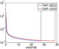
(a) $L_{1}$

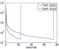
(b) group lasso

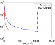
(c) fused lasso

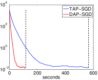
(d) nuclear norm

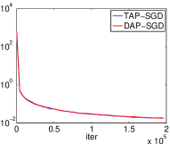
(e) $L_{1}$

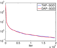
(f) group lasso

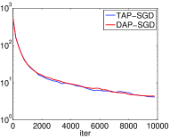
(g) fused lasso

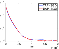
(h) nuclear norm

Figure 1: Comparison of TAP-SGD and DAP-SGD in terms of time and number of iterations. The Y-axis shows the log distance between the solution generated by an algorithm and the optimal solution, denoted by $\log\|\mathbf{x}-\mathbf{x}^{*}\|_{2}^{2}$. Results of $L_{1}$, group lasso, simplified fused lasso and nuclear norm regularized objectives are shown in columns from left to right, respectively. Top and bottom rows correspond to the results regarding time and number of iterations, respectively.

We compare the proposed DAP-SGD algorithm with TAP-SGD in a consistent way without assuming the data is sparse. The implementation is based on the single machine multi-core system (shared memory architecture). Both algorithms are implemented in C++ and run on a multi-core server. Singular value decomposition (SVD) is calculated by eigen3. The parameters are locked while they are being updated. The lock operation will slow down the computation; however it guarantees that the implementation conforms to the algorithm and its corresponding convergence analysis.

Without loss of generality, we choose the least square loss with a non-smooth regularization term as the optimization objective:

$$\begin{split}\min_{\mathbf{x}\in\mathbb{R}^{m}}P(\mathbf{x})=f(\mathbf{x})+h(\mathbf{x})=\frac{1}{n}\sum_{i=1}^{n}\left[\|\mathbf{x}^{\mathrm{T}}\mathbf{s}_{i}-y_{i}\|_{2}^{2}+\lambda\|\mathbf{x}\|_{2}^{2}\right]+h(\mathbf{x})\end{split}.$$ (22)

In the case of nuclear norm regularization, the loss function $f(\mathbf{x})$ becomes the multi-target least square loss $f(\mathbf{X})=\frac{1}{n}\sum_{i=1}^{n}\left[\|\mathbf{X}^{\mathrm{T}}\mathbf{s}_{i}-\mathbf{y}_{i}\|_{2}^{2}+\lambda\|\mathbf{X}\|_{F}^{2}\right]$ correspondingly.

In the implementation TAP-SGD, the proximal operator of the $L_{1}$ regularized objective can be parallelized easily, while the proximal operators of group lasso, simplified fused lasso and nuclear norm are not parallelized due to their coupled and non-element-wise operations. On the other hand, the procedure of the master in the proposed DAP-SGD only involves simple element-wise operations.

Experimental Setup. We conduct two experiments to evaluate the algorithms with 4 different non-smooth regularization terms ($L_{1}$, group lasso, simplified fused lasso, nuclear norm) regarding the running time and number of iterations, as well as the speedup. Data is generated randomly. In the first experiment, for the 4 different objectives, the number of samples $n$ is set to $1\times 10^{3}$, $1\times 10^{3}$, $1\times 10^{3}$, and $4\times 10^{3}$, while the length of the parameter is set to $5\times 10^{3}$, $5\times 10^{3}$, $5\times 10^{3}$ and $2\times 10^{3}$ (in the form of a $50\times 40$ matrix for nuclear norm regularization), respectively. The number of iterations $T$ is set to $2\times 10^{5}$, $2\times 10^{5}$, $1\times 10^{4}$ and $2\times 10^{4}$, and the step-size $\eta_{t}$ is set to $\frac{1}{2\times 10^{5}+200t}$, $\frac{1}{2\times 10^{5}+200t}$, $\frac{1}{2\times 10^{5}+200t}$ and $\frac{1}{2\times 10^{4}+t}$, respectively, which is decreasing with iterations. The hyper-parameter $\lambda$ is set to $200$, $200$, $200$, $0.1$ correspondingly. In the second experiment of evaluating the speedup, the settings are identical to the first experiment except that the number of iterations for simplified fused norm and nuclear norm regularized objectives is set to $10^{4}$ and $2\times 10^{4}$, and the number of parameters for $L_{1}$ and group lasso regularized objectives is set to $5\times 10^{4}$. The total time cost of a system consists of two parts: evaluation of updating information in the workers and updating in the master. If we can speed up both with $k$ times, then we can achieve a $k$-speed up in the ideal case. In our experiment, the number of updating threads running in parallel and maximum delay $\tau$ in the master is fixed to the number of workers.

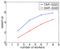
(a) $L_{1}$

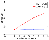
(b) group lasso

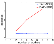
(c) fused lasso

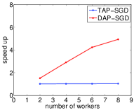
(d) nuclear norm

Figure 2: Speedup of TAP-SGD and DAP-SGD with 4 different non-smooth regularization terms.

Results are summarized in Figures 1 and 2. Figure 1 shows the comparison between TAP-SGD and DAP-SGD regarding the running time and number of iterations. As shown in the top row of Figure 1, the proposed DAP-GSD algorithm is slightly slower than TAP-SGD with the $L_{1}$ regularized objective. The reason is that the proximal operator of $L_{1}$ norm is element-wise and can be parallelized. The decoupled update of DAP-SGD (8) involves more operations in workers than the update of TAP-SGD (3), whose workers only need to evaluate the gradients. Nevertheless, DAP-SGD is much faster than TAP-SGD with group lasso, simplified fused lasso and nuclear norm regularized objectives because the proximal operators of these norms are not element-wise and hard to parallelize. As a consequence, evaluation of the proximal operator in the master of TAP-SGD becomes the computational bottleneck of the whole system and the performance degrades significantly. In contrast, DAP-SGD allows each worker to evaluate the proximal operator, which justifies our core idea of decoupling the computation. Meanwhile, according to the bottom row of Figure 1, TAP-SGD and DAP-SGD perform similarly regarding the number of iterations. The experimental results shown in Figure 1 validate that the decoupled operation in DAP-SGD makes the algorithm more flexible and easier to parallelize without affecting the precision of the algorithm.

Figure 2 compares TAP-SGD and DAP-SGD in terms of the speedup with different regularization terms. Obviously, DAP-SGD can achieve significant speedup with the number of workers increasing except for the $L_{1}$ regularized objective due to the same reason discussed above. With group lasso, simplified fused lasso and nuclear norm regularized objectives, TAP-SGD essentially fails to speedup when the number of workers increases, which indicates the computational bottleneck at the master for evaluating the coupled proximal operator. Meanwhile, the decoupling operation of DAP-SGD is effective to off-load the computation to the workers and improves the parallelism in asynchronous proximal stochastic gradient descent.

6 Conclusion

This paper proposes a novel decoupled asynchronous proximal stochastic gradient descent (DAP-SGD) algorithm for optimizing a composite objective function. By off-loading computation from the master to workers, the proposed DAP-SGD algorithm becomes easy to parallelize. DAP-SGD is suitable for many master-worker architectures, including single machine multi-core systems and multi-machine systems. We further provide theoretical convergence analyses for DAP-SGD, with both diminishing and fixed step-sizes.

Appendix for Make Workers Work Harder: Decoupled Asynchronous Proximal Stochastic Gradient Descent

Theorem 1

Suppose that the cost function of (1) satisfies the following conditions: $f(\mathbf{x})$ is strongly convex with constant $\mu$ and $h(\mathbf{x})$ is convex; $f(\mathbf{x})$ is differentiable and $\triangledown\!f(\mathbf{x})$ is Lipschitz continuous with constant $L$; $\mathbb{E}\|\triangledown\!f_{i}(\mathbf{x})-\triangledown\!f(\mathbf{x})\|_{2}^{2}\leq C_{f}$; $\|\partial h(\mathbf{x})\|_{2}^{2}\leq C_{h}$. Define the optimal solution of (1) as $\mathbf{x}^{*}$. At time $t$, set the step-size of the DAP-SGD recursion (8) as $\eta_{t}=O(1/t)$. Then the iterate generated by (8) at time $T$, denoted by $\mathbf{x}_{T}$, satisfies

$$\begin{split}\mathbb{E}\|\mathbf{x}_{T}-\mathbf{x}^{*}\|_{2}^{2}\leq O\left(\frac{\log T}{T}\right).\end{split}$$ (23)

Proof of Theorem 1: From the DAP-SGD update $\mathbf{x}_{t+1}=\mathbf{x}_{t}+\mathbf{x}_{d(t)}^{\prime}-\mathbf{x}_{d(t)}$, we have

$$\begin{split}&\mathbb{E}\|\mathbf{x}_{t+1}-\mathbf{x}^{*}\|_{2}^{2}\\ =&\mathbb{E}\|\mathbf{x}_{t}-\mathbf{x}^{*}+\mathbf{x}_{d(t)}^{\prime}-\mathbf{x}_{d(t)}\|^{2}\\ =&\mathbb{E}\|\mathbf{x}_{t}-\mathbf{x}^{*}\|_{2}^{2}+\mathbb{E}\|\mathbf{x}_{d(t)}^{\prime}-\mathbf{x}_{d(t)}\|^{2}+2\mathbb{E}\left<\mathbf{x}_{d(t)}^{\prime}-\mathbf{x}_{d(t)},\mathbf{x}_{t}-\mathbf{x}^{*}\right>\\ =&\mathbb{E}\|\mathbf{x}_{t}-\mathbf{x}^{*}\|_{2}^{2}+\underbrace{\mathbb{E}\|\mathbf{x}_{d(t)}^{\prime}-\mathbf{x}_{d(t)}\|^{2}+2\mathbb{E}\left<\mathbf{x}_{d(t)}^{\prime}-\mathbf{x}_{d(t)},\mathbf{x}_{d(t)}-\mathbf{x}^{*}\right>}_{\mathrm{Q}_{1}}+2\mathbb{E}\left<\mathbf{x}_{d(t)}^{\prime}-\mathbf{x}_{d(t)},\mathbf{x}_{t}-\mathbf{x}_{d(t)}\right>.\end{split}$$ (24)

Below we bound the value of $\mathrm{Q}_{1}$ from above.

Recalling the update of $\mathbf{x}^{\prime}_{d(t)}$ in (8) of the paper, which is

$$\begin{split}\mathbf{x}^{\prime}_{d(t)}&=\text{Prox}_{\eta,h}(\mathbf{x}_{d(t)}-\eta_{d(t)}\triangledown\!f_{i_{d(t)}}(\mathbf{x}_{d(t)}))\\ &=\arg\!\min_{\mathbf{y}}\frac{1}{2\eta_{d(t)}}\|\mathbf{y}-(\mathbf{x}_{d(t)}-\eta_{d(t)}\triangledown\!f_{i_{d(t)}}(\mathbf{x}_{d(t)}))\|_{2}^{2}+h(\mathbf{y}),\end{split}$$ (25)

we have

$$\begin{split}\frac{1}{\eta_{d(t)}}(\mathbf{x}_{d(t)}-\mathbf{x}^{\prime}_{d(t)})-\triangledown f_{i_{d(t)}}(\mathbf{x}_{d(t)})\in\partial h(\mathbf{x}^{\prime}_{d(t)}).\end{split}$$ (26)

Because $f(\mathbf{x})$ is convex (right now we do not need to use its strong convexity) and $h(\mathbf{x})$ is also convex, we have the following lower bound for the optimal value

$$\begin{split}P(\mathbf{x}^{*})\triangleq&f(\mathbf{x}^{*})+h(\mathbf{x}^{*})\\ \geq&f(\mathbf{x}_{d(t)})+\left<\triangledown\!f(\mathbf{x}_{d(t)}),\mathbf{x}^{*}-\mathbf{x}_{d(t)}\right>+h(\mathbf{x}^{\prime}_{d(t)})+\left<\partial h(\mathbf{x}^{\prime}_{d(t)}),\mathbf{x}^{*}-\mathbf{x}^{\prime}_{d(t)}\right>.\\ \end{split}$$ (27)

With a slight abuse of notation, here and thereafter $\partial h(\mathbf{x}^{\prime}_{d(t)})$ stands for any subgradient. Hence we substitute the one given in (26) into (27) and obtain

$$\begin{split}P(\mathbf{x}^{*})\geq&f(\mathbf{x}_{d(t)})+\left<\triangledown\!f(\mathbf{x}_{d(t)}),\mathbf{x}^{*}-\mathbf{x}_{d(t)}\right>\\ &+h(\mathbf{x}^{\prime}_{d(t)})+\left<\frac{1}{\eta_{d(t)}}(\mathbf{x}_{d(t)}-\mathbf{x}^{\prime}_{d(t)})-\triangledown\!f_{i_{d(t)}}(\mathbf{x}_{d(t)}),\mathbf{x}^{*}-\mathbf{x}^{\prime}_{d(t)}\right>.\end{split}$$ (28)

On the other hand, $\triangledown\!f(\mathbf{x})$ being Lipschitz continuous with constant $L$ implies

$$\begin{split}f(\mathbf{x}^{\prime}_{d(t)})\leq f(\mathbf{x}_{d(t)})+\left<\triangledown\!f(\mathbf{x}_{d(t)}),\mathbf{x}^{\prime}_{d(t)}-\mathbf{x}_{d(t)}\right>+\frac{L}{2}\|\mathbf{x}^{\prime}_{d(t)}-\mathbf{x}_{d(t)}\|_{2}^{2}.\end{split}$$ (29)

Substituting (29) into (28)

$$\begin{split}P(\mathbf{x}^{*})\geq&f(\mathbf{x}^{\prime}_{d(t)})-\left<\triangledown\!f(\mathbf{x}_{d(t)}),\mathbf{x}^{\prime}_{d(t)}-\mathbf{x}_{d(t)}\right>-\frac{L}{2}\|\mathbf{x}^{\prime}_{d(t)}-\mathbf{x}_{d(t)}\|_{2}^{2}+\left<\triangledown\!f(\mathbf{x}_{d(t)}),\mathbf{x}^{*}-\mathbf{x}_{d(t)}\right>\\ &+h(\mathbf{x}^{\prime}_{d(t)})+\left<\frac{1}{\eta_{d(t)}}(\mathbf{x}_{d(t)}-\mathbf{x}^{\prime}_{d(t)})-\triangledown\!f_{i_{d(t)}}(\mathbf{x}_{d(t)}),\mathbf{x}^{*}-\mathbf{x}^{\prime}_{d(t)}\right>.\end{split}$$ (30)

Noticing that by definition $P(\mathbf{x}^{\prime}_{d(t)})\triangleq f(\mathbf{x}^{\prime}_{d(t)})+h(\mathbf{x}^{\prime}_{d(t)})$ and reorganizing the terms of (30), we obtain

$$\begin{split}-[P(\mathbf{x}^{\prime}_{d(t)})-P(\mathbf{x}^{*})]\geq&\left<\triangledown\!f(\mathbf{x}_{d(t)})-\triangledown\!f_{i_{d(t)}}(\mathbf{x}_{d(t)}),\mathbf{x}^{*}-\mathbf{x}^{\prime}_{d(t)}\right>+\frac{1}{\eta_{d(t)}}\left<\mathbf{x}_{d(t)}-\mathbf{x}^{\prime}_{d(t)},\mathbf{x}^{*}-\mathbf{x}_{d(t)}\right>\\ &+\frac{1}{\eta_{d(t)}}\|\mathbf{x}_{d(t)}-\mathbf{x}^{\prime}_{d(t)}\|^{2}-\frac{L}{2}\|\mathbf{x}_{d(t)}-\mathbf{x}^{\prime}_{d(t)}\|^{2}.\end{split}$$ (31)

Assuming that $\eta_{t}\leq 1/L$ for any $t$ (this assumption holds according to the step-size rule given later), (31) yields

$$\begin{split}-[P(\mathbf{x}^{\prime}_{d(t)})-P(\mathbf{x}^{*})]\geq&\left<\triangledown\!f(\mathbf{x}_{d(t)})-\triangledown\!f_{i_{d(t)}}(\mathbf{x}_{d(t)}),\mathbf{x}^{*}-\mathbf{x}^{\prime}_{d(t)}\right>+\frac{1}{\eta_{d(t)}}\left<\mathbf{x}_{d(t)}-\mathbf{x}^{\prime}_{d(t)},\mathbf{x}^{*}-\mathbf{x}_{d(t)}\right>\\ &+\frac{1}{2\eta_{d(t)}}\|\mathbf{x}_{d(t)}-\mathbf{x}^{\prime}_{d(t)}\|^{2}.\end{split}$$ (32)

Taking expectation on both sides of (32) and reorganizing terms, we have

$$\begin{split}&-\mathbb{E}[P(\mathbf{x}^{\prime}_{d(t)})-P(\mathbf{x}^{*})]+\underbrace{\mathbb{E}\left<\triangledown\!f_{i_{d(t)}}(\mathbf{x}_{d(t)})-\triangledown\!f(\mathbf{x}_{d(t)}),\mathbf{x}^{*}-\mathbf{x}^{\prime}_{d(t)}\right>}_{\mathrm{Q}_{2}}\\ \geq&\frac{1}{\eta_{d(t)}}\mathbb{E}\left<\mathbf{x}_{d(t)}-\mathbf{x}^{\prime}_{d(t)},\mathbf{x}^{*}-\mathbf{x}_{d(t)}\right>+\frac{1}{2\eta_{d(t)}}\mathbb{E}\|\mathbf{x}_{d(t)}-\mathbf{x}^{\prime}_{d(t)}\|^{2}.\end{split}$$ (33)

Define $\hat{\mathbf{x}}^{\prime}_{d(t)}\triangleq\text{Prox}_{\eta,h}(\mathbf{x}_{d(t)}-\eta_{d(t)}\triangledown\!f(\mathbf{x}_{d(t)}))$ as an approximation of $\mathbf{x}^{\prime}_{d(t)}\triangleq\text{Prox}_{\eta,h}(\mathbf{x}_{d(t)}-\eta_{d(t)}\triangledown\!f_{i_{d(t)}}(\mathbf{x}_{d(t)}))$. Because the random variable $i_{d(t)}$ is independent with $\mathbf{x}^{*}$ and $\hat{\mathbf{x}}^{\prime}_{d(t)}$, while $\mathbb{E}\left[\triangledown\!f_{i_{d(t)}}(\mathbf{x}_{d(t)})\right]=\triangledown\!f(\mathbf{x}_{d(t)})$, it holds $\mathbb{E}\langle\triangledown\!f_{i_{d(t)}}(\mathbf{x}_{d(t)})-\triangledown\!f(\mathbf{x}_{d(t)}),\mathbf{x}^{*}-\hat{\mathbf{x}}^{\prime}_{d(t)}\rangle=0$. Hence, $\mathrm{Q}_{2}$ can be upper bounded by

$$\begin{split}Q_{2}=&\mathbb{E}\left<\triangledown\!f_{i_{d(t)}}(\mathbf{x}_{d(t)})-\triangledown\!f(\mathbf{x}_{d(t)}),\mathbf{x}^{*}-\mathbf{x}^{\prime}_{d(t)}\right>\\ =&\mathbb{E}\left<\triangledown\!f_{i_{d(t)}}(\mathbf{x}_{d(t)})-\triangledown\!f(\mathbf{x}_{d(t)}),\mathbf{x}^{*}-\hat{\mathbf{x}}^{\prime}_{d(t)}\right>+\mathbb{E}\left<\triangledown\!f_{i_{d(t)}}(\mathbf{x}_{d(t)})-\triangledown\!f(\mathbf{x}_{d(t)}),\hat{\mathbf{x}}^{\prime}_{d(t)}-\mathbf{x}^{\prime}_{d(t)}\right>\\ =&\mathbb{E}\left<\triangledown\!f_{i_{d(t)}}(\mathbf{x}_{d(t)})-\triangledown\!f(\mathbf{x}_{d(t)}),\hat{\mathbf{x}}^{\prime}_{d(t)}-\mathbf{x}^{\prime}_{d(t)}\right>\\ \leq&\mathbb{E}\left(\|\triangledown\!f_{i_{d(t)}}(\mathbf{x}_{d(t)})-\triangledown\!f(\mathbf{x}_{d(t)})\|_{2}\|\hat{\mathbf{x}}^{\prime}_{d(t)}-\mathbf{x}^{\prime}_{d(t)}\|_{2}\right),\end{split}$$ (34)

where the last inequality comes from the Cauchy-Schwarz inequality. Further, the non-expansive property of proximal operators [8] implies

$$\begin{split}\|\hat{\mathbf{x}}^{\prime}_{d(t)}-\mathbf{x}^{\prime}_{d(t)}\|_{2}=&\|\text{Prox}_{\eta,h}(\mathbf{x}_{d(t)}-\eta_{d(t)}\triangledown\!f(\mathbf{x}_{d(t)}))-\text{Prox}_{\eta,h}(\mathbf{x}_{d(t)}-\eta_{d(t)}\triangledown\!f_{i_{d(t)}}(\mathbf{x}_{d(t)}))\|_{2}\\ \leq&\eta_{d(t)}\|\triangledown\!f_{i_{d(t)}}(\mathbf{x}_{d(t)})-\triangledown\!f(\mathbf{x}_{d(t)})\|_{2}.\end{split}$$ (35)

Combining (34) and (35) yields an upper bound of $Q_{2}$ as

$$\begin{split}Q_{2}\leq\eta_{d(t)}\mathbb{E}\|\triangledown\!f_{i_{d(t)}}(\mathbf{x}_{d(t)})-\triangledown\!f(\mathbf{x}_{d(t)})\|_{2}^{2}\leq\eta_{d(t)}C_{f},\end{split}$$ (36)

where the last inequality is due to the assumption of bounded variance $\mathbb{E}\|\triangledown\!f_{i}(\mathbf{x})-\triangledown\!f(\mathbf{x})\|_{2}^{2}\leq C_{f}$.

Substituting (36) into (33), we have

$$\begin{split}&-\mathbb{E}[P(\mathbf{x}^{\prime}_{d(t)})-P(\mathbf{x}^{*})]+\eta_{d(t)}C_{f}\\ \geq&\frac{1}{\eta_{d(t)}}\mathbb{E}\left<\mathbf{x}_{d(t)}-\mathbf{x}^{\prime}_{d(t)},\mathbf{x}^{*}-\mathbf{x}_{d(t)}\right>+\frac{1}{2\eta_{d(t)}}\mathbb{E}\|\mathbf{x}_{d(t)}-\mathbf{x}^{\prime}_{d(t)}\|^{2}.\end{split}$$ (37)

Now we end up with an upper bound of $\mathrm{Q}_{1}$ as

$$\begin{split}\mathrm{Q}_{1}\triangleq&\mathbb{E}\|\mathbf{x}_{d(t)}^{\prime}-\mathbf{x}_{d(t)}\|^{2}+2\mathbb{E}\left<\mathbf{x}_{d(t)}^{\prime}-\mathbf{x}_{d(t)},\mathbf{x}_{d(t)}-\mathbf{x}^{*}\right>\\ \leq&-2\eta_{d(t)}\mathbb{E}[P(\mathbf{x}^{\prime}_{d(t)})-P(\mathbf{x}^{*})]+2\eta_{d(t)}^{2}C_{f}.\end{split}$$ (38)

Therefore

$$\begin{split}\mathrm{Q}_{1}\leq&-2\eta_{d(t)}\mathbb{E}[P(\mathbf{x}_{t})-P(\mathbf{x}^{*})]-2\eta_{d(t)}\mathbb{E}[P(\mathbf{x}^{\prime}_{d(t)})-P(\mathbf{x}_{t})]+2\eta_{d(t)}^{2}C_{f}.\\ \leq&-\mu\eta_{d(t)}\mathbb{E}\|\mathbf{x}_{t}-\mathbf{x}^{*}\|_{2}^{2}-2\eta_{d(t)}\mathbb{E}[P(\mathbf{x}^{\prime}_{d(t)})-P(\mathbf{x}_{t})]+2\eta_{d(t)}^{2}C_{f}.\end{split}$$ (39)

The second line comes from the inequality

$$\begin{split}P(\mathbf{x}_{t})-P(\mathbf{x}^{*})\geq\frac{\mu}{2}\|\mathbf{x}_{t}-\mathbf{x}^{*}\|_{2}^{2},\end{split}$$ (40)

which is due to the facts that $\mathbf{x}^{*}$ is the optimal solution of $P(\mathbf{x})=f(\mathbf{x})+h(\mathbf{x})$, $f(\mathbf{x})$ is strongly convex with constant $\mu$, and $h(\mathbf{x})$ is convex.

Substituting (39) into (24), we have

$$\begin{split}\mathbb{E}\|\mathbf{x}_{t+1}-\mathbf{x}^{*}\|_{2}^{2}\leq&(1-\mu\eta_{d(t)})\mathbb{E}\|\mathbf{x}_{t}-\mathbf{x}^{*}\|_{2}^{2}+2\eta_{d(t)}\underbrace{\mathbb{E}[P(\mathbf{x}_{d(t)})-P(\mathbf{x}^{\prime}_{d(t)})]}_{\mathrm{Q}_{3}}\\ &+2\eta_{d(t)}\sum_{p=1}^{t-d(t)}\underbrace{\mathbb{E}[P(\mathbf{x}_{t-p+1})-P(\mathbf{x}_{t-p})]}_{\mathrm{Q}_{4}}+2\eta_{d(t)}^{2}C_{f}+2\underbrace{\mathbb{E}\left<\mathbf{x}_{d(t)}^{\prime}-\mathbf{x}_{d(t)},\mathbf{x}_{t}-\mathbf{x}_{d(t)}\right>}_{\mathrm{Q}_{5}}.\end{split}$$ (41)

We proceed to bound the terms $\mathrm{Q}_{3}$, $\mathrm{Q}_{4}$, and $\mathrm{Q}_{5}$.

Because $f(\mathbf{x})$ and $h(\mathbf{x})$ are convex as well as the norm of $\partial h(\mathbf{x})$ is bounded, we have the following basic inequality

$$\begin{split}P(\mathbf{x})-P(\mathbf{y})=&f(\mathbf{x})-f(\mathbf{y})+h(\mathbf{x})-h(\mathbf{y})\\ \leq&\left<\triangledown\!f(\mathbf{x}),\mathbf{x}-\mathbf{y}\right>+\left<\partial h(\mathbf{x}),\mathbf{x}-\mathbf{y}\right>\\ \leq&\|\triangledown\!f(\mathbf{x})\|_{2}\|\mathbf{x}-\mathbf{y}\|_{2}+\|\partial h(\mathbf{x})\|_{2}\|\mathbf{x}-\mathbf{y}\|_{2}\\ \leq&\|\triangledown\!f(\mathbf{x})\|_{2}\|\mathbf{x}-\mathbf{y}\|_{2}+\sqrt{C_{h}}\|\mathbf{x}-\mathbf{y}\|_{2}\\ =&(\|\triangledown\!f(\mathbf{x})\|_{2}+\sqrt{C_{h}})\|\mathbf{x}-\mathbf{y}\|_{2}.\end{split}$$ (42)

In (42), the second line comes from the convexity of $f(\mathbf{x})$ and $h(\mathbf{x})$, while the third line comes from the Cauchy-Schwarz inequality. Replacing $\mathbf{x}$ by $\mathbf{x}_{d(t)}$ and $\mathbf{y}$ by $\mathbf{x}^{\prime}_{d(t)}$ in (42), we have

$$\begin{split}\mathrm{Q}_{3}=\mathbb{E}\left[P(\mathbf{x}_{d(t)})-P(\mathbf{x}^{\prime}_{d(t)})\right]\leq\mathbb{E}\left[(\|\triangledown f(\mathbf{x}_{d(t)})\|_{2}+\sqrt{C_{h}})\|\mathbf{x}_{d(t)}-\mathbf{x}^{\prime}_{d(t)}\|_{2}\right].\end{split}$$ (43)

Applying the expression of $\mathbf{x}_{d(t)}-\mathbf{x}^{\prime}_{d(t)}$ in (26) into (43) yields

$$\begin{split}\mathrm{Q}_{3}\leq&\eta_{d(t)}\mathbb{E}\left[(\|\triangledown\!f(\mathbf{x}_{d(t)})\|_{2}+\sqrt{C_{h}})\|\triangledown\!f_{i_{d(t)}}(\mathbf{x}_{d(t)})+\partial h(\mathbf{x}^{\prime}_{d(t)})\|_{2}\right]\\ \leq&\frac{1}{2}\eta_{d(t)}\mathbb{E}\|\triangledown\!f(\mathbf{x}_{d(t)})\|_{2}^{2}+\frac{1}{2}\eta_{d(t)}C_{h}+\eta_{d(t)}\mathbb{E}\|\triangledown\!f_{i_{d(t)}}(\mathbf{x}_{d(t)})+\partial h(\mathbf{x}^{\prime}_{d(t)})\|_{2}^{2}.\end{split}$$ (44)

Due to the inequalities

$$\begin{split}\frac{1}{2}\|\triangledown\!f(\mathbf{x}_{d(t)})\|_{2}^{2}\leq\|\triangledown\!f(\mathbf{x}_{d(t)})-\triangledown\!f(\mathbf{x}^{*})\|_{2}^{2}+\|\triangledown\!f(\mathbf{x}^{*})\|_{2}^{2},\end{split}$$ (45)

and

$$\begin{split}&\|\triangledown\!f_{i_{d(t)}}(\mathbf{x}_{d(t)})+\partial h(\mathbf{x}^{\prime}_{d(t)})\|_{2}^{2}\\ \leq&2\|\triangledown\!f_{i_{d(t)}}(\mathbf{x}_{d(t)})\|_{2}^{2}+2\|\partial h(\mathbf{x}^{\prime}_{d(t)})\|_{2}^{2}\\ \leq&4\|\triangledown\!f_{i_{d(t)}}(\mathbf{x}_{d(t)})-\triangledown\!f(\mathbf{x}_{d(t)})\|_{2}^{2}+4\|\triangledown\!f(\mathbf{x}_{d(t)})\|_{2}^{2}+2\|\partial h(\mathbf{x}^{\prime}_{d(t)})\|_{2}^{2}\\ \leq&4\|\triangledown\!f_{i_{d(t)}}(\mathbf{x}_{d(t)})-\triangledown\!f(\mathbf{x}_{d(t)})\|_{2}^{2}+8\|\triangledown\!f(\mathbf{x}_{d(t)})-\triangledown f(\mathbf{x}^{*})\|_{2}^{2}+8\|\triangledown\!f(\mathbf{x}^{*})\|_{2}^{2}+2\|\partial h(\mathbf{x}^{\prime}_{d(t)})\|_{2}^{2},\end{split}$$ (46)

(44) turns to

$$\begin{split}\mathrm{Q}_{3}\leq&9\eta_{d(t)}\mathbb{E}\|\triangledown\!f(\mathbf{x}_{d(t)})-\triangledown\!f(\mathbf{x}^{*})\|_{2}^{2}+9\eta_{d(t)}\mathbb{E}\|\triangledown\!f(\mathbf{x}^{*})\|_{2}^{2}+4\eta_{d(t)}\mathbb{E}\|\triangledown\!f_{i_{d(t)}}(\mathbf{x}_{d(t)})-\triangledown\!f(\mathbf{x}_{d(t)})\|_{2}^{2}\\ &+2\eta_{d(t)}\mathbb{E}\|\partial h(\mathbf{x}^{\prime}_{d(t)})\|_{2}^{2}+\frac{1}{2}\eta_{d(t)}C_{h}.\\ \end{split}$$ (47)

Considering Lipschitz continuity of $\triangledown\!f(\mathbf{x})$, $\|\triangledown\!f(\mathbf{x}^{*})\|_{2}^{2}\leq C_{h}$ from Corollary 1, $\mathbb{E}\|\triangledown\!f_{i}(\mathbf{x})-\triangledown\!f(\mathbf{x})\|_{2}^{2}\leq C_{f}$, as well as $\|\partial h(\mathbf{x})\|_{2}^{2}\leq C_{h}$, (47) further turns to

$$\begin{split}\mathrm{Q}_{3}\leq 9\eta_{d(t)}L^{2}\mathbb{E}\|\mathbf{x}_{d(t)}-\mathbf{x}^{*}\|_{2}^{2}+4\eta_{d(t)}C_{f}+\frac{23}{2}\eta_{d(t)}C_{h}.\end{split}$$ (48)

Similar to the derivation of (48), we have

$$\begin{split}\mathrm{Q}_{4}=&\mathbb{E}\left[P(\mathbf{x}_{t-p+1})-P(\mathbf{x}_{t-p})\right]\\ \leq&\mathbb{E}\left[(\|\triangledown f(\mathbf{x}_{t-p+1})\|_{2}+\sqrt{C_{h}})\|\mathbf{x}_{t-p+1}-\mathbf{x}_{t-p}\|_{2}\right]\\ \leq&\eta_{d(t-p)}\mathbb{E}\left[(\|\triangledown\!f(\mathbf{x}_{t-p+1})\|_{2}+\sqrt{C_{h}})\|\triangledown\!f_{i_{d(t-p)}}(\mathbf{x}_{d(t-p)})+\partial h(\mathbf{x}^{\prime}_{d(t-p)})\|_{2}\right]\\ \leq&\frac{1}{2}\eta_{d(t-p)}\mathbb{E}\|\triangledown\!f(\mathbf{x}_{t-p+1})\|_{2}^{2}+\frac{1}{2}\eta_{d(t-p)}C_{h}+\eta_{d(t-p)}\mathbb{E}\|\triangledown\!f_{i_{d(t-p)}}(\mathbf{x}_{d(t-p)})+\partial h(\mathbf{x}^{\prime}_{d(t-p)})\|_{2}^{2}.\end{split}$$ (49)

Using the inequalities (see (45) and (46))

$$\begin{split}\frac{1}{2}\|\triangledown\!f(\mathbf{x}_{t-p+1})\|_{2}^{2}\leq\|\triangledown\!f(\mathbf{x}_{t-p+1})-\triangledown\!f(\mathbf{x}^{*})\|_{2}^{2}+\|\triangledown\!f(\mathbf{x}^{*})\|_{2}^{2},\end{split}$$ (50)

and

$$\begin{split}&\|\triangledown\!f_{i_{d(t-p)}}(\mathbf{x}_{d(t-p)})+\partial h(\mathbf{x}^{\prime}_{d(t-p)})\|_{2}^{2}\\ \leq&4\|\triangledown\!f_{i_{d(t-p)}}(\mathbf{x}_{d(t-p)})-\triangledown\!f(\mathbf{x}_{d(t-p)})\|_{2}^{2}+8\|\triangledown\!f(\mathbf{x}_{d(t-p)})-\triangledown\!f(\mathbf{x}^{*})\|_{2}^{2}+8\|\triangledown\!f(\mathbf{x}^{*})\|_{2}^{2}+2\|\partial h(\mathbf{x}^{\prime}_{d(t-p)})\|_{2}^{2},\end{split}$$ (51)

(49) yields

$$\begin{split}\mathrm{Q}_{4}\leq&\eta_{d(t-p)}\mathbb{E}\|\triangledown\!f(\mathbf{x}_{t-p+1})-\triangledown\!f(\mathbf{x}^{*})\|_{2}^{2}+9\eta_{d(t-p)}\mathbb{E}\|\triangledown\!f(\mathbf{x}^{*})\|^{2}+8\eta_{d(t-p)}\mathbb{E}\|\triangledown\!f(\mathbf{x}_{t-p})-\triangledown\!f(\mathbf{x}^{*})\|_{2}^{2}\\ &+4\eta_{d(t-p)}\mathbb{E}\|\triangledown\!f_{i_{d(t-p)}}(\mathbf{x}_{d(t-p)})-\triangledown\!f(\mathbf{x}_{d(t-p)})\|_{2}^{2}+2\eta_{d(t-p)}\mathbb{E}\|\partial h(\mathbf{x}^{\prime}_{d(t-p)})\|_{2}^{2}+\frac{1}{2}\eta_{d(t-p)}C_{h}\\ \leq&\eta_{d(t-p)}L^{2}\mathbb{E}\|\mathbf{x}_{t-p+1}-\mathbf{x}^{*}\|_{2}^{2}+8\eta_{d(t-p)}L^{2}\mathbb{E}\|\mathbf{x}_{d(t-p)}-\mathbf{x}^{*}\|_{2}^{2}+4\eta_{d(t-p)}C_{f}+\frac{23}{2}\eta_{d(t-p)}C_{h}.\end{split}$$ (52)

Again, the last line of (52) utilizes Lipschitz continuity of $\triangledown\!f(x)$, $\|\triangledown\!f(\mathbf{x}^{*})\|_{2}^{2}\leq C_{h}$ from Corollary 1, $\mathbb{E}\|\triangledown\!f_{i}(\mathbf{x})-\triangledown\!f(\mathbf{x})\|_{2}^{2}\leq C_{f}$, as well as $\|\partial h(\mathbf{x})\|_{2}^{2}\leq C_{h}$.

For the term $Q_{5}$, we use the Cauchy-Schwarz inequality followed by the substitution of (26) and get

$$\begin{split}\mathrm{Q}_{5}=&\mathbb{E}\left<\mathbf{x}_{d(t)}^{\prime}-\mathbf{x}_{d(t)},\mathbf{x}_{t}-\mathbf{x}_{d(t)}\right>\\ \leq&\mathbb{E}\left(\|\mathbf{x}_{d(t)}^{\prime}-\mathbf{x}_{d(t)}\|_{2}\|\mathbf{x}_{t}-\mathbf{x}_{d(t)}\|_{2}\right)\\ \leq&\eta_{d(t)}\mathbb{E}\left(\|\triangledown\!f_{i_{d(t)}}(\mathbf{x}_{d(t)})+\partial h(\mathbf{x}^{\prime}_{d(t)})\|_{2}\|\mathbf{x}_{t}-\mathbf{x}_{d(t)}\|_{2}\right).\\ \end{split}$$ (53)

Further relaxing (53) by the triangle inequality yields

$$\begin{split}\mathrm{Q}_{5}\leq\eta_{d(t)}\sum_{p=1}^{t-d(t)}\mathbb{E}\left(\|\triangledown\!f_{i_{d(t)}}(\mathbf{x}_{d(t)})+\partial h(\mathbf{x}^{\prime}_{d(t)})\|_{2}\|\mathbf{x}_{t-p+1}-\mathbf{x}_{t-p}\|_{2}\right).\end{split}$$ (54)

Since the maximum delay is $\tau$, we have

$$\begin{split}\mathrm{Q}_{5}\leq\eta_{d(t)}\sum_{p=1}^{\tau}\mathbb{E}\left(\|\triangledown\!f_{i_{d(t)}}(\mathbf{x}_{d(t)})+\partial h(\mathbf{x}^{\prime}_{d(t)})\|_{2}\|\mathbf{x}_{t-p+1}-\mathbf{x}_{t-p}\|_{2}\right).\\ \end{split}$$ (55)

Noticing the relations $\mathbf{x}_{t-p+1}-\mathbf{x}_{t-p}=\mathbf{x}^{\prime}_{d(t-p)}-\mathbf{x}_{d(t-p)}$ from the DAP-SGD recursion and $\mathbf{x}^{\prime}_{d(t-p)}-\mathbf{x}_{d(t-p)}=\eta_{d(t)}(\triangledown\!f(\mathbf{x}_{d(t-p)})+\partial h(\mathbf{x}^{\prime}_{d(t-p)}))$ from (26), (56) leads to

$$\begin{split}\mathrm{Q}_{5}\leq\eta_{d(t)}\sum_{p=1}^{\tau}\eta_{d(t-p)}\mathbb{E}\left(\|\triangledown\!f_{i_{d(t)}}(\mathbf{x}_{d(t)})+\partial h(\mathbf{x}^{\prime}_{d(t)})\|_{2}\|\triangledown\!f(\mathbf{x}_{d(t-p)})+\partial h(\mathbf{x}^{\prime}_{d(t-p)})\|_{2}\right).\end{split}$$ (56)

Following the similar routines as those in (48) and (52), eventually we reach

$$\begin{split}\mathrm{Q}_{5}\leq&4\eta_{d(t)}L^{2}\sum_{p=1}^{\tau}\eta_{d(t-p)}\mathbb{E}\|\mathbf{x}_{d(t)}-\mathbf{x}^{*}\|_{2}^{2}+4\eta_{d(t)}L^{2}\sum_{p=1}^{\tau}\eta_{d(t-p)}\mathbb{E}\|\mathbf{x}_{d(t-p)}-\mathbf{x}^{*}\|_{2}^{2}\\ &+4\eta_{d(t)}\sum_{p=1}^{\tau}\eta_{d(t-p)}C_{f}+10\eta_{d(t)}\sum_{p=1}^{\tau}\eta_{d(t-p)}C_{h}\end{split}$$ (57)

Substituting (48), (52) and (57) into (41), we have

$$\begin{split}\mathbb{E}\|\mathbf{x}_{t+1}-\mathbf{x}^{*}\|_{2}^{2}\leq&\left(1-\mu\eta_{d(t)}\right)\mathbb{E}\|\mathbf{x}_{t}-\mathbf{x}^{*}\|_{2}^{2}+\left(8\eta_{d(t)}L^{2}\sum_{p=1}^{\tau}\eta_{d(t-p)}+18\eta_{d(t)}^{2}L^{2}\right)\mathbb{E}\|\mathbf{x}_{d(t)}-\mathbf{x}^{*}\|_{2}^{2}\\ &+2\eta_{d(t)}L^{2}\sum_{p=1}^{\tau}\eta_{d(t-p)}\mathbb{E}\|\mathbf{x}_{t-p+1}-\mathbf{x}^{*}\|_{2}^{2}+24\eta_{d(t)}L^{2}\sum_{p=1}^{\tau}\eta_{d(t-p)}\mathbb{E}\|\mathbf{x}_{d(t-p)}-\mathbf{x}^{*}\|_{2}^{2}\\ &+\left(16\eta_{d(t)}\sum_{p=1}^{\tau}\eta_{d(t-p)}+8\eta_{d(t)}^{2}\right)C_{f}+\left(43\eta_{d(t)}\sum_{p=1}^{\tau}\eta_{d(t-p)}+23\eta_{d(t)}^{2}\right)C_{h}.\end{split}$$ (58)

Define the step-size rule

$$\begin{split}\eta_{t}=\frac{1}{\mu(t+1)+u}=O\left(\frac{1}{t}\right),\end{split}$$ (59)

where $u$ is a positive constant satisfying:

• $u>(2\tau-1)\mu$ such that $\eta_{t}\leq\eta_{d(t)}$;

• $u$ is large enough such that $\min(\mu/(4C_{1}\tau),1/L)\geq\eta_{t}$, where $C_{1}$ is a constant we give below.

Define two constants

$$C_{1}=\left(2L^{2}\frac{\mu+u}{\mu+u-2\mu\tau}+48\tau L^{2}+8\tau L^{2}\frac{\mu+u}{\mu+u-2\mu\tau}\right)\frac{\mu+u}{\mu+u-\mu\tau}+18L^{2},$$

and

$$C_{2}=\left[(16\tau+8)C_{f}+(43\tau+23)C_{h}\right]\frac{(\mu+u)^{2}}{{(\mu+u-2\mu\tau)}^{2}}.$$

Though not straightforward, we can show that under the step-size rule given by (59), (58) yields

$$\begin{split}\mathbb{E}\|\mathbf{x}_{t+1}-\mathbf{x}^{*}\|_{2}^{2}\leq(1-\mu\eta_{t})\mathbb{E}\|\mathbf{x}_{t}-\mathbf{x}^{*}\|_{2}^{2}+C_{1}\sum_{p=0}^{2\tau}\eta_{t-p}^{2}\mathbb{E}\|\mathbf{x}_{t-p}-\mathbf{x}^{*}\|_{2}^{2}+C_{2}\eta_{t}^{2}.\end{split}$$ (60)

For the ease of presentation, we define $a_{t}=\mathbb{E}\|\mathbf{x}_{t}-\mathbf{x}^{*}\|_{2}^{2}$ and will analyze its rate. Rewrite (60) to

$$\begin{split}a_{t+1}\leq(1-\mu\eta_{t})a_{t}+C_{1}\sum_{p=0}^{2\tau}\eta_{t-p}^{2}a_{t-p}+C_{2}\eta_{t}^{2}.\end{split}$$ (61)

Applying telescopic cancellation to (61) from $t=0$ to $t=T-1$ yields

$$\begin{split}a_{T}\leq&a_{0}-\sum_{t=0}^{T-1}\mu\eta_{t}a_{t}+C_{1}\sum_{t=0}^{T-1}\sum_{p=0}^{2\tau}\eta_{t-p}^{2}a_{t-p}+C_{2}\sum_{t=0}^{T-1}\eta_{t}^{2}\\ \leq&a_{0}-\sum_{t=0}^{T-1}(\mu\eta_{t}-2C_{1}\eta_{t}^{2}\tau)a_{t}+C_{2}O(1).\end{split}$$ (62)

As we can verify, $\mu/(4C_{1}\tau)\geq\eta_{t}$, meaning that

$$\begin{split}\sum_{t=0}^{T-1}(\mu\eta_{t}-2C_{1}\eta_{t}^{2}\tau)a_{t}\geq\frac{1}{2}\sum_{t=0}^{T-1}\mu\eta_{t}a_{t}.\end{split}$$ (63)

Combining (62) and (63), we have

$$\begin{split}\frac{1}{2}\sum_{t=0}^{T-1}\mu\eta_{t}a_{t}\leq a_{0}-a_{T}+C_{2}O(1),\end{split}$$ (64)

which, along with the step-size rule (59), implies that

$$\begin{split}\sum_{t=0}^{T-1}\frac{1}{\mu(t+1)+u}a_{t}\leq\frac{2}{\mu}(a_{0}+C_{2}O(1))\end{split}$$ (65)

Further define $C_{3}=u/(u-\mu\tau)$ such that

$$\frac{\mu(t+1)+u}{(\mu(t-p+1)+u)^{2}}\leq\frac{C_{3}}{\mu(t-p+1)+u}.$$

Substituting the step-size rule (59) into (61), we have

$$\begin{split}a_{t+1}\leq&\left(1-\frac{\mu}{\mu(t+1)+u}\right)a_{t}+C_{1}\sum_{p=0}^{2\tau}\frac{1}{(\mu(t-p+1)+u)^{2}}a_{t-p}+\frac{1}{(\mu(t+1)+u)^{2}}C_{2},\end{split}$$ (66)

and consequently

$$\begin{split}(\mu(t+1)+u)a_{t+1}\leq&(\mu t+u)a_{t}+C_{1}\sum_{p=0}^{2\tau}\frac{\mu(t+1)+u}{(\mu(t-p+1)+u)^{2}}a_{t-p}+\frac{1}{\mu(t+1)+u}C_{2}\\ \leq&(\mu t+u)a_{t}+C_{1}C_{3}\sum_{p=0}^{2\tau}\frac{1}{\mu(t-p+1)+u}a_{t-p}+\frac{1}{\mu(t+1)+u}C_{2}.\end{split}$$ (67)

Applying telescopic cancellation again to (67) from $t=0$ to $t=T-1$, we have

$$\begin{split}(\mu T+u)a_{T}\leq&ua_{0}+C_{1}C_{3}\sum_{t=0}^{T-1}\sum_{p=0}^{2\tau}\frac{1}{\mu(t-p+1)+u}a_{t-p}+\sum_{t=0}^{T-1}\frac{1}{\mu(t+1)+u}C_{2}\\ \leq&ua_{0}+2C_{1}C_{3}\tau\sum_{t=0}^{T-1}\frac{1}{\mu(t+1)+u}a_{t}+\sum_{t=0}^{T-1}\frac{1}{\mu(t+1)+u}C_{2}.\end{split}$$ (68)

Substituting (65) into (68) yields

$$\begin{split}(\mu T+u)a_{T}\leq ua_{0}+\frac{4}{\mu}C_{1}C_{3}\tau(a_{0}+C_{2}O(1))+C_{2}O(\log T),\end{split}$$ (69)

and consequently

$$\begin{split}a_{T}\leq\frac{ua_{0}+\frac{4}{\mu}C_{1}C_{3}\tau(a_{0}+C_{2}O(1))+C_{2}O(\log T)}{\mu T+u}=O\left(\frac{\log T}{T}\right),\end{split}$$ (70)

which completes the proof.

 

Theorem 2

Suppose that the cost function of (1) satisfies the following conditions: $f(\mathbf{x})$ is strongly convex with constant $\mu$ and $h(\mathbf{x})$ is convex; $f(\mathbf{x})$ is differentiable and $\triangledown\!f(\mathbf{x})$ is Lipschitz continuous with constant $L$; $\mathbb{E}\|\triangledown\!f_{i}(\mathbf{x})-\triangledown\!f(\mathbf{x})\|_{2}^{2}\leq C_{f}$; $\|\partial h(\mathbf{x})\|_{2}^{2}\leq C_{h}$. Define the optimal solution of (1) as $\mathbf{x}^{*}$. At time $t$, fix the step-size of the DAP-SGD recursion (8) $\eta_{t}$ as $\eta=O(1/\sqrt{T})$, where $T$ is the maximum number of iterations. Define the iterate generated by (8) at time $t$ as $\mathbf{x}_{t}$. Then the running average iterate generated by (8) at time $T$, denoted by

$$\bar{\mathbf{x}}_{T}=\frac{1}{T+1}\sum_{t=0}^{T}\mathbf{x}_{t},$$

satisfies

$$\begin{split}\mathbb{E}\|\bar{\mathbf{x}}_{T}-\mathbf{x}^{*}\|_{2}^{2}\leq O\left(\frac{1}{\sqrt{T}}\right).\end{split}$$ (71)

Proof of Theorem 2: We start from (58) in the proof of Theorem 1. Define the step-size rule

$$\begin{split}\eta_{t}=\eta=\frac{1}{v\sqrt{T}},\end{split}$$ (72)

where $v$ is a positive constant such that $\min(\mu/(4C_{4}\tau),1/L)\geq\eta$. Defining constants

$$C_{4}=(2+56\tau)L^{2},$$

and

$$C_{5}=(16\tau+8)C_{f}+(43\tau+23)C_{h},$$

followed by manipulating (58), we have (similar to the inequality (61)) the following result

$$\begin{split}a_{t+1}\leq(1-\mu\eta)a_{t}+C_{4}\eta^{2}\sum_{p=0}^{2\tau}a_{t-p}+C_{5}\eta^{2}\end{split}$$ (73)

Applying telescopic cancellation to (73) from $t=0$ to $t=T$ yields

$$\begin{split}a_{T+1}\leq&a_{0}-\sum_{t=0}^{T}\mu\eta a_{t}+C_{4}\eta^{2}\sum_{t=0}^{T}\sum_{p=0}^{2\tau}a_{t-p}+C_{5}(T+1)\eta^{2}\\ \leq&a_{0}-\sum_{t=0}^{T}(\mu\eta-2C_{4}\eta^{2}\tau)a_{t}+C_{5}(T+1)\eta^{2}.\end{split}$$ (74)

Since $\mu/(4C_{4}\tau)\geq\eta$ such that

$$\begin{split}\sum_{t=0}^{T}(\mu\eta-2C_{4}\tau\eta^{2})a_{t}\geq\frac{\mu\eta}{2}\sum_{t=0}^{T}a_{t},\end{split}$$ (75)

(74) implies

$$\begin{split}\frac{\mu\eta}{2}\sum_{t=0}^{T}a_{t}\leq&a_{0}-a_{T+1}+C_{5}(T+1)\eta^{2},\end{split}$$ (76)

and consequently

$$\begin{split}\frac{\mu\eta}{T+1}\sum_{t=0}^{T}a_{t}\leq&\frac{2a_{0}+2C_{5}(T+1)\eta^{2}}{T+1}.\end{split}$$ (77)

According to Jensen’s inequality, we have

$$\begin{split}\frac{\mu\eta}{T+1}\sum_{t=0}^{T}a_{t}=&\frac{\mu\eta}{T+1}\sum_{t=0}^{T}\mathbb{E}\|\mathbf{x}_{t}-\mathbf{x}^{*}\|_{2}^{2}\\ \geq&\mu\eta\mathbb{E}\left\|\frac{1}{T+1}\sum_{t=0}^{T}\mathbf{x}_{t}-\mathbf{x}^{*}\right\|_{2}^{2}\\ =&\mu\eta\mathbb{E}\|\bar{\mathbf{x}}_{T}-\mathbf{x}^{*}\|_{2}^{2}.\end{split}$$ (78)

Substituting (78) and the step-size rule (72) into (77), we have

$$\begin{split}\mathbb{E}\|\bar{\mathbf{x}}_{T}-\mathbf{x}^{*}\|_{2}^{2}\leq&\frac{2a_{0}v\sqrt{T}+2C_{5}(T+1)\frac{1}{v\sqrt{T}}}{\mu(T+1)}=O(\frac{1}{\sqrt{T}}),\end{split}$$ (79)

which completes the proof.

References

• [1] F.Β Niu, B.Β Recht, C.Β Re, S.Β J. Wright, Hogwild: A lock-free approach to parallelizing stochastic gradient descent, in: Proceedings of Advances in Neural Information Processing Systems 24, December 12-14, 2011, Granada, Spain, 2011, pp. 693–701.
• [2] A.Β Agarwal, J.Β C. Duchi, Distributed delayed stochastic optimization, in: Proceedings of Advances in Neural Information Processing Systems 24, December 12-14, 2011, Granada, Spain, 2011, pp. 873–881.
• [3] M.Β Li, D.Β G. Andersen, A.Β J. Smola, K.Β Yu, Communication efficient distributed machine learning with the parameter server, in: Proceedings of Advances in Neural Information Processing Systems 27, December 8-13 2014, Montreal, Quebec, Canada, 2014, pp. 19–27.
• [4] X.Β Lian, Y.Β Huang, Y.Β Li, J.Β Liu, Asynchronous parallel stochastic gradient for nonconvex optimization, in: Proceedings of Advances in Neural Information Processing Systems 28, December 7-12, 2015, Montreal, Quebec, Canada, 2015, pp. 2737–2745.
• [5] R.Β Zhang, J.Β T. Kwok, Asynchronous distributed ADMM for consensus optimization, in: Proceedings of the 31th International Conference on Machine Learning, ICML 2014, Beijing, China, 21-26 June 2014, 2014, pp. 1701–1709.
• [6] H.Β R. Feyzmahdavian, A.Β Aytekin, M.Β Johansson, A delayed proximal gradient method with linear convergence rate, in: IEEE International Workshop on Machine Learning for Signal Processing, MLSP 2014, Reims, France, September 21-24, 2014, pp. 1–6.
• [7] J.Β Liu, S.Β J. Wright, C.Β RΓ©, V.Β Bittorf, S.Β Sridhar, An asynchronous parallel stochastic coordinate descent algorithm, Journal of Machine Learning Research 16 (2015) 285–322.
• [8] J.Β Liu, S.Β J. Wright, Asynchronous stochastic coordinate descent: Parallelism and convergence properties, SIAM Journal on Optimization 25Β (1) (2015) 351–376.
• [9] O.Β Fercoq, P.Β RichtΓ‘rik, Accelerated, parallel, and proximal coordinate descent, SIAM Journal on Optimization 25Β (4) (2015) 1997–2023.
• [10] J.Β Mareček, P.Β RichtΓ‘rik, M.Β TakÑč, Distributed block coordinate descent for minimizing partially separable functions, in: Numerical Analysis and Optimization, Springer, 2015, pp. 261–288.
• [11] M.Β Hong, A distributed, asynchronous and incremental algorithm for nonconvex optimization: An admm based approach, arXiv preprint arXiv:1412.6058.
• [12] Y.Β Zhou, Y.Β Yu, W.Β Dai, Y.Β Liang, E.Β Xing, On convergence of model parallel proximal gradient algorithm for stale synchronous parallel system, in: International Conference on Artificial Intelligence and Statistics (AISTATS), 2016.
• [13] C.Β Hsieh, H.Β Yu, I.Β S. Dhillon, Passcode: Parallel asynchronous stochastic dual co-ordinate descent, in: Proceedings of the 32nd International Conference on Machine Learning, ICML 2015, Lille, France, 6-11 July 2015, 2015, pp. 2370–2379.
• [14] A.Β Beck, M.Β Teboulle, A fast iterative shrinkage-thresholding algorithm for linear inverse problems, SIAM journal on imaging sciences 2Β (1) (2009) 183–202.
• [15] N.Β Parikh, S.Β P. Boyd, Proximal algorithms., Foundations and Trends in optimization 1Β (3) (2014) 127–239.
• [16] J.Β Friedman, T.Β Hastie, R.Β Tibshirani, A note on the group lasso and a sparse group lasso, arXiv preprint arXiv:1001.0736.
• [17] J.Β Liu, L.Β Yuan, J.Β Ye, An efficient algorithm for a class of fused lasso problems, in: Proceedings of the 16th ACM SIGKDD International Conference on Knowledge Discovery and Data Mining, Washington, DC, USA, July 25-28, 2010, 2010, pp. 323–332.
• [18] S.Β Ji, J.Β Ye, An accelerated gradient method for trace norm minimization, in: Proceedings of the 26th Annual International Conference on Machine Learning, ICML 2009, Montreal, Quebec, Canada, June 14-18, 2009, 2009, pp. 457–464.
• [19] J.Β Cai, E.Β J. CandΓ¨s, Z.Β Shen, A singular value thresholding algorithm for matrix completion, SIAM Journal on Optimization 20Β (4) (2010) 1956–1982.
• [20] Y.Β Nesterov, Introductory lectures on convex optimization: A basic course, Vol.Β 87, Springer Science & Business Media, 2013.
• [21] A.Β Nemirovski, A.Β Juditsky, G.Β Lan, A.Β Shapiro, Robust stochastic approximation approach to stochastic programming, SIAM Journal on Optimization 19Β (4) (2009) 1574–1609.