Local Matrix Homotopies and Soft Tori

Abstract.

We present solutions to local connectivity problems in matrix representations of the form $C([-1,1]^{N})\to A_{n,\varepsilon}\leftarrow C_{\varepsilon}(\mathbb{T}^{2})$ for any $\varepsilon\in[0,2]$ and any integer $n\geq 1$, where $A_{n,\varepsilon}\subseteq M_{n}$ and where $C_{\varepsilon}(\mathbb{T}^{2})$ denotes the Soft Torus. We solve the connectivity problems by introducing the so called toroidal matrix links, which can be interpreted as normal contractive matrix analogies of free homotopies in differential algebraic topology.

In order to deal with the locality constraints, we have combined some techniques introduced in this document with some techniques from matrix geometry, combinatorial optimization, classification and representation theory of C^∗-algebras.

1. Introduction

In this document we study the solvability of some local connectivity problems via constrained normal matrix homotopies in C^∗-representations of the form

(1.1) $$C({\mathbb{T}^{N}})\longrightarrow M_{n},$$

for a fixed but arbitrary integer $N\geq 1$ and any integer $n\geq 1$. In particular we study local normal matrix homotopies which preserve commutativity and also satisfy some additional constraints, like being rectifiable or piecewise analytic.

We build on some homotopic techniques introduced initially by Bratteli, Elliot, Evans and Kishimoto in [3] and generalized by Lin in [18] and [22]. We combine the homotopic techniques with some techniques introduced here and some other techniques from matrix geometry and noncommutative topology developed by Loring [24, 27], Shulman [27], Bhatia [1], Chu [7], Brockett [4], Choi [6, 5], Effros [5], Exel [10], Eilers [10], Elsner [11], Pryde [30, 29], McIntosh [29] and Ricker [29], to construct the so called toroidal matrix links, which we use to obtain the main theorems presented in section §4, and which consist on local connectivity results in matrix representations of the form 1.1 and also of the form

(1.2) $$C({\mathbb{T}^{N}})\longrightarrow M_{n}\longleftarrow C([-1,1]^{N}).$$

Toroidal matrix links can be interpreted as noncommutative analogies of free homotopies in algebraic topology and topological deformation theory, they are introduced in section §3 together with some other matrix geometrical objects.

In §4.3 we present a connectivity technique which provides us with very important imformation on the local uniform connectivity in matrix representations of the form $C({\mathbb{T}^{2}})\to M_{n}$.

Given $\delta>0$, a function $\varepsilon:\mathbb{R}\to\mathbb{R}^{+}_{0}$ and two matrices $x,y$ in a set $S\subseteq M_{n}$ such that $\|x-y\|\leq\delta$, by a $\varepsilon(\delta)$-local matrix homotopy between $x$ and $y$, we mean a matrix path $X\in C([0,1],M_{n})$ such that $X_{0}=x$, $X_{1}=y$, $X_{t}\in S$ and $\|X_{t}-y\|\leq\varepsilon(\delta)$ for each $t\in[0,1]$. We write $x\rightsquigarrow_{\varepsilon}y$ to denote that there is a $\varepsilon$-local matrix homotopy betweeen $x$ and $y$.

The motivation and inspiration to study local normal matrix homotopies which preserve commutativity in C^∗-representations of the form 1.1 and 1.2, came from mathematical physics [15, §3] and matrix approximation theory [8].

The problems from mathematical physics which motivated this study are inverse spectral problems, which consist on finding for a certain set of matrices $X_{1},\ldots,X_{N}$ which approximately satisfy a set of polynomial constraints $\mathcal{R}(x_{1},\ldots,$ $x_{N})$ on $N$ NC-variables, a set of nearby matrices $\tilde{X}_{1},\ldots,\tilde{X}_{N}$ which approximate $X_{1},\ldots,X_{N}$ and exactly satisfy the constraints $\mathcal{R}(x_{1},\ldots,x_{N})$. The problems from matrix approximation theory that we considered for this study, are of the type that can be reduced to the study of the solvability conditions for approximate and exact joint diagonalization problems for $N$-tuples of normal matrix contractions.

Since the problems which motivated the research reported in this document can be restated in terms of the study local piecewise analytic connectivity in matrix representations of the form $C_{\varepsilon}({\mathbb{T}^{2}})\to M_{n}\leftarrow C({\mathbb{T}^{N}})$ and $C_{\varepsilon}({\mathbb{T}^{2}})\to M_{n}\leftarrow C([-1,1]^{N})$, we studied several variations of problems of the form.

Problem 1 (Lifted connectivity problem).

Given $\varepsilon>0$, is there $\delta>0$ such that the following conditions hold? For any integer $n\geq 1$, some prescribed sequence of linear compressions $\kappa_{n}:M_{mn}\to M_{n}$ for some $m\geq 1$, and any two families of $N$ pairwise commuting normal contractions $X_{1},\ldots,X_{N}$ and $Y_{1},\ldots,Y_{N}$ in $M_{n}$ which satisfy the constraints $\|X_{j}-Y_{j}\|\leq\delta$, $1\leq j\leq N$, there are two families of $N$ pairwise commuting normal contractions $\tilde{X}_{1},\ldots,\tilde{X}_{N}$ and $\tilde{Y}_{1},\ldots,\tilde{Y}_{N}$ in $M_{mn}$ which satisfy the relations: $\kappa(\tilde{X}_{j})=X_{j}$, $\kappa(\tilde{Y}_{j})=Y_{j}$ and $\|\tilde{X}_{j}-\tilde{Y}_{j}\|\leq\varepsilon$, $1\leq j\leq N$. Moreover, there are $N$ peicewise analytic $\varepsilon$-local homotopies of normal contractions $\mathbf{X}^{1},\ldots,\mathbf{X}^{N}\in C([0,1],M_{mn})$ between the corresponding pairs $\tilde{X}_{j}$, $\tilde{Y}_{j}$ in $M_{mn}$, which satisfy the relations $\mathbf{X}_{t}^{j}\mathbf{X}_{t}^{k}=\mathbf{X}_{t}^{k}\mathbf{X}_{t}^{j}$, for each $1\leq j,k\leq N$ and each $0\leq t\leq 1$.

By solving problem P.1 we learned about the local connectivity of arbitrary $\delta$-close $N$-tuples of pairwise commuting normal contractions $X_{1},\ldots,X_{N}$ and $Y_{1},\ldots,$ $Y_{N}$ in $M_{n}$, which was the main motivation of the research reported here. We also obtained some results concerning to the geometric structure of the joint spectra (in the sense of [29]) of the $N$-tuples.

For a given $\delta>0$, the study of the solvability conditions of problems of the form P.1 provided us with geometric information about local deformations of particular representations of the form $C({\mathbb{T}^{N}})\to A_{0}:=C^{*}(U_{1},\ldots,U_{N})\subseteq M_{n}$ and $C({\mathbb{T}^{N}})\to A_{1}:=C^{*}(V_{1},\ldots,V_{N})\subseteq M_{n}$, where $U_{1},\ldots,U_{N},V_{1},\ldots,V_{N}\in\mathbb{U}(n)$ are pairwise commuting unitary matrices such that $\|U_{j}-V_{j}\|\leq\delta$. By local deformations we mean a family $\{A_{t}\}_{t\in[0,1]}\subseteq M_{n}$ of abelian C^∗-algebras, with $A_{t}:=C^{*}(\mathbf{X}_{t}^{1},\ldots,\mathbf{X}_{t}^{N})$ and where $\mathbf{X}_{t}^{1},\ldots,\mathbf{X}_{t}^{N}\in C([0,1],\mathbb{U}(n))$ are $\varepsilon(\delta)$-local matrix homotopies between $U_{1},\ldots,U_{N}$ and $V_{1},\ldots,V_{N}$ for some function $\varepsilon:\mathbb{R}\to\mathbb{R}^{+}_{0}$.

The main results are presented in §4, in section §4.2 we use toroidal matrix links to obtain some local piecewise analytic connectivity results which are non-uniform in dimension. In section §4.2.1 we derive an uniform approximate connectivity technique via matrix homotopy lifting and in section §4.4 we present a connectivity lemma that can be used to derive some uniform connectivity results betweeen matrix representations of finite sets of universal algebraic contractions, some of the details of these constructions will be presented in [33].

2. Preliminaries and Notation

2.1. Matrix Sets and Operations

Given two elements $x,y$ in a C^∗-algebra $A$, we will write $[x,y]$ and $\mathrm{Ad}[x](y)$ to denote the operations $[x,y]:=xy-yx$ and $\mathrm{Ad}[x](y):=xyx^{*}$.

Given any C^∗-algebra $A$ and any element $x$ in $M_{n}(A)$, we will denote by $\mathrm{diag}_{n}\left[x\right]$ the operation defined by the expression

$$M_{n}(A) \rightarrow M_{n}(A)$$

$$x \mapsto \mathrm{diag}_{n}\left[x\right]$$

$$\left(\begin{array}[]{cccc}x_{11}&x_{12}&\cdots&x_{1n}\\ x_{21}&x_{22}&\cdots&x_{2n}\\ \vdots&\vdots&\ddots&\vdots\\ x_{n1}&x_{n2}&\cdots&x_{nn}\end{array}\right) \mapsto \left(\begin{array}[]{cccc}x_{11}&0&\cdots&0\\ 0&x_{22}&\cdots&0\\ \vdots&\vdots&\ddots&\vdots\\ 0&0&\cdots&x_{nn}\end{array}\right).$$

Given a C^∗-algebra $A$, we write $\mathcal{N}(A)$, $\mathbb{H}(A)$ and $\mathbb{U}(A)$ to denote the sets of normal, hermitian and unitary elements in $A$ respectively. We will write $\mathcal{N}(n)$, $\mathbb{H}(n)$ and $\mathbb{U}(n)$ instead of $\mathcal{N}(M_{n})$, $\mathbb{H}(M_{n})$ and $\mathbb{U}(M_{n})$. A normal element $u$ in a C^∗-algebra $A$ is called a partial unitary if the element $uu^{*}=p$ is an otrhogonal projection in $A$, i.e. $p$ satisfies the relations $p=p^{*}=p^{2}$, we denote by $\mathbb{PU}(A)$ the set of partial unitaries in $A$ and we write $\mathbb{PU}(n)$ instead of $\mathbb{PU}(M_{n})$.

We write $\mathbb{I}$, $\mathbb{J}$, ${\mathbb{T}^{1}}$ and ${\mathbb{D}^{2}}$ to denote the sets $\mathbb{I}:=[0,1]$, $\mathbb{J}=[-1,1]$, ${\mathbb{T}^{1}}:=\{z\in\mathbb{C}|\>|z|=1\}$ and ${\mathbb{D}^{2}}:=\{z\in\mathbb{C}|\>|z|\leq 1\}$. For some arbitrary matrix set $S\subseteq M_{n}$ and some arbitrary compact set $\mathbb{X}\subset\mathbb{C}$, we will write $S(\mathbb{X})$ to denote the subset of elements in $S$ described by the expression,

(2.2) $$S(\mathbb{X}):=\{x\in S|\sigma(x)\subseteq\mathbb{X}\},$$

for instance we can write $\mathcal{N}(n)({\mathbb{D}^{2}})$ to denote the set of nomal contractions. We will denote by $\mathcal{M}_{\infty}$ the C^∗-algebra described by

(2.3) $$\mathcal{M}_{\infty}:=\overline{\bigcup_{n\in\mathbb{Z}^{+}}M_{n}}^{\|\cdot\|}.$$

In this document we write $\mathbb{1}_{n}$ to denote the identity matrix in $M_{n}$. The symbol $\mathbf{N}_{n}$ will be used to denote the diagonal matrices

(2.4) $$\mathbf{N}_{n}:=\mathrm{diag}\left[n,n-1,\ldots,2,1\right].$$

We will write $\Omega_{n}$ and $\Sigma_{n}$ to denote the unitary matrices defined by

(2.5) $$\Omega_{n}:=e^{\frac{2\pi i}{n}\mathbf{N}_{n}} = \mathrm{diag}\left[1,e^{\frac{2\pi i(n-1)}{n}},\ldots,e^{\frac{4\pi i}{n}},e^{\frac{2\pi i}{n}}\right]$$

and

(2.8) $$\Sigma_{n} := \left(\begin{array}[]{cc}0&\mathbb{1}_{n-1}\\ 1&0\end{array}\right).$$

Remark 2.1.

The unitary matrices $\Omega_{n}$ and $\Sigma_{n}$ are related, by the equation

$$\Omega_{n}=\mathscr{F}_{n}^{*}\Sigma_{n}\mathscr{F}_{n},$$

where $\mathscr{F}_{N}:=\left(\frac{1}{\sqrt{N}}e^{\frac{2\pi i(j-1)(k-1)}{N}}\right)_{1\leq j,k\leq N}$ is the discrete Fourier transform (DFT) unitary matrix.

Given an abstract object (group or C^∗-algebra) $A$ we write $A^{\ast N}$ to denote the operation consisting on taking the free product of $N$ copies of $A$.

Definition 2.1 (Local preservers).

Given a linear mapping $K:M_{N}\to M_{n}$, with $n\leq N$, and given a set $S\subseteq M_{n}$, we say that $K$ locally preserves $S$ if there is $T\subseteq M_{N}$ such that $K(T)\subseteq S$, if in particular $K(T)\subseteq\mathcal{N}(n)$ we say that $K$ locally preserves normality.

Example 2.1.

The linear compression $\kappa:M_{2n}\to M_{n}$ defined by

$$\kappa:\left(\begin{array}[]{cc}x_{11}&x_{12}\\ x_{21}&x_{22}\end{array}\right)\mapsto x_{11}$$

locally preserves normality with respect to the set $T:=\{X\in M_{2n}|x_{11}\in\mathcal{N}(n)\}$.

Example 2.2.

The linear map $\phi:M_{n}\to M_{n},x\mapsto\mathbf{D}x$ with $n\geq 1$ and $\mathbf{D}=\frac{1}{n}\mathrm{diag}\left[1,\ldots,n\right]$, locally preserves commutativity with respect to the set $C^{*}(\mathbf{D})$.

2.2. Joint Spectral Variation

2.2.1. Clifford Operators

Using the same notation as Pryde in [30], let $\mathbb{R}_{(N)}$ denote the Clifford algebra over $\mathbb{R}$ with generators $e_{1},\ldots,e_{N}$ and relations $e_{i}e_{j}=-e_{j}e_{i}$ for $i\neq j$ and $e^{2}_{i}=-1$. Then $\mathbb{R}_{(N)}$ is an associative algebra of dimension $2^{N}$. Let $S(N)$ denote the set $\mathscr{P}(\{1,\ldots,N\})$. Then the elements $e_{S}=e_{s_{1}}\cdots e_{s_{k}}$ form a basis when $S=\{s_{1},\ldots,s_{k}\}$ and $1\leq s_{1}<\cdots<s_{k}\leq N$. Elements of $\mathbb{R}_{(N)}$ are denoted by $\lambda=\sum_{S}\lambda_{S}e_{S}$ where $\lambda_{S}\in\mathbb{R}$. Under the inner product $\scalprod*{\lambda}{\mu}=\sum_{S}\lambda_{S}\mu_{S}$, $\mathbb{R}_{(N)}$ becomes a Hilbert space with orthonormal basis $\{e_{S}\}$.

The Clifford operator of $N$ elements $X_{1},\ldots,X_{N}\in M_{n}$ is the operator defined in $M_{n}\otimes\mathbb{R}_{(N)}$ by

$$\mathrm{Cliff}(X_{1},\ldots,X_{N}):=i\sum_{j=1}^{N}X_{j}\otimes e_{j}.$$

Each element $T=\sum_{S}T_{S}\otimes e_{S}\in M_{n}\otimes\mathbb{R}_{(N)}$ acts on elements $x=\sum_{S}x_{S}\otimes e_{S}\in\mathbb{C}^{n}\otimes\mathbb{R}_{(N)}$ by $T(x):=\sum_{S,S^{\prime}}T_{s}(x_{S^{\prime}})\otimes e_{S}e_{S^{\prime}}$. So $\mathrm{Cliff}(X_{1},\ldots,X_{N})\in M_{n}\otimes\mathbb{R}_{(N)}\subseteq\mathcal{L}(\mathbb{C}^{n}\otimes\mathbb{R}_{(N)})$. By $\|\mathrm{Cliff}(X_{1},\ldots,X_{N})\|$ we will mean the operator norm of $\mathrm{Cliff}(X_{1},\ldots,X_{N})$ as an element of $\mathcal{L}(\mathbb{C}^{n}\otimes\mathbb{R}_{(N)})$. As observed by Elsner in [11, 5.2] we have that

(2.9) $$\|\mathrm{Cliff}(X_{1},\ldots,X_{N})\|\leq\sum_{j=1}^{N}\|X_{j}\|.$$

2.2.2. Joint Spectral Matchings

It is often convenient to have $N$-tuples (or $2N$-tuples) of matrices with real spectra. For this purpose we use the following construction, initiated by McIntosh and Pryde. If $X=(X_{1},\ldots,X_{N})$ is a $N$-tuple of $n$ by $n$ matrices then we can always decompose $X_{j}$ in the form $X_{j}=X_{1j}+iX_{2j}$ where the $X_{kj}$ all have real spectra. We write $\pi(X):=(X_{11},\ldots,X_{1N},X_{21},\ldots,X_{2N})$ and call $\pi(X)$ a partition of $X$. If the $X_{kj}$ all commute we say that $\pi(X)$ is a commuting partition, and if the $X_{kj}$ are simultaneously triangularizable $\pi(X)$ is a triangularizable partition. If the $X_{kj}$ are all semisimple (diagonalizable) then $\pi(X)$ is called a semisimple partition.

We say that $N$ normal matrices $X_{1},\ldots,X_{N}\in M_{n}$ are simultaneously diagonalizable if there is a unitary matrix $Q\in M_{n}$ such that $Q^{*}X_{j}Q$ is diagonal for each $j=1,\ldots,N$. In this case, for $1\leq k\leq n$, let $\Lambda^{(k)}(X_{j}):=(Q^{*}X_{j}Q)_{kk}$ the $(k,k)$ element of $Q^{*}X_{j}Q$, and set $\Lambda^{(k)}(X_{1},\ldots,X_{N}):=(\Lambda^{(k)}(X_{1}),\ldots,\Lambda^{(k)}(X_{N}))\in\mathbb{C}^{N}$. The set

$$\Lambda(X_{1},\ldots,X_{N}):=\{\Lambda^{(k)}(X_{1},\ldots,X_{N})\}_{1\leq k\leq N}$$

is called the joint spectrum of $X_{1},\ldots,X_{N}$. We will write $\Lambda(X_{j})$ to denote the $j$-component of $\Lambda(X_{1},\ldots,X_{N})$, in other words we will have that

$$\Lambda(X_{j})=\mathrm{diag}\left[\Lambda^{(1)}(X_{j}),\ldots,\Lambda^{(N)}(X_{j})\right].$$

The following theorem was proved in McIntosh, Pryde and Ricker [29].

Theorem 2.1 (McIntosh, Pryde and Ricker).

Let $X=(X_{1},\ldots,X_{N})$ and $Y=(Y_{1},\ldots,$ $Y_{N})$ be $N$-tuples of commuting $n$ by $n$ normal matrices. There exists a permutation $\tau$ of the index set $\{1,\ldots,n\}$ such that

(2.10) $$\|\Lambda^{(k)}(X_{1},\ldots,X_{N})-\Lambda^{(\tau(k))}(Y_{1},\ldots,Y_{N})\|\leq e_{N,0}\|\mathrm{Cliff}(X_{1}-Y_{1},\ldots,X_{N}-Y_{N})\|$$

for all $k\in\{1,\ldots,n\}$.

In this theorem, $e_{N,0}$ is an explicit constant depending only on $N$ defined in [29, (2.4)].

2.3. Amenable C^∗-algebras and Bott elements

The following lemma has been proved by H. Lin in [19].

Lemma 2.1 (H. Lin.).

For any $\varepsilon>0$ and $d>0$, there exists $\delta>0$ satisfying the following: Suppose that $A$ is a unital C^∗-algebra and $u\in A$ is a unitary such that ${\mathbb{T}^{1}}\backslash\sigma(u)$ contains an arc with length $d$. Suppose that $a\in A$ with $\|a\|\leq 1$ such that

$$\|ua-au\|<\delta.$$

Then there is a self-adjoint element $h\in A$ such that $u=e^{ih}$,

$$\|ha-ah\|<\varepsilon\>\>\>\>\mathrm{and}\>\>\>\>\|e^{ith}a-ae^{ith}\|<\varepsilon$$

for all $t\in\mathbb{I}$. If, furthermore, $a=p$ is a projection, we have

$$\left\|pup-p+\sum_{n=1}^{\infty}\frac{(iphp)^{n}}{n!}\right\|<\varepsilon.$$

The following lemma was proved by H. Lin in [22] using L.2.1, since for any integer $n\geq 1$ and any $u\in\mathbb{U}(n)$, we will have that ${\mathbb{T}^{1}}\backslash\sigma(u)$ contains an arc with length at least $2\pi/n$.

Lemma 2.2 (H. Lin.).

Let $\varepsilon>0$, $n\geq 1$ be an integer and $M>0$. There exists $\delta>0$ satisfying the following: For any finite set $\mathscr{F}\subset M_{n}$ with $\|a\|\leq M$ for all $a\in\mathscr{F}$, and a unitary $u\in M_{n}$ such that

$$\|ua-au\|<\delta\>\>\>\>\mathrm{for\>\>all}\>\>\>\>a\in\mathscr{F},$$

there exists a continuous path of unitaries $\{u(t)\}_{t\in\mathbb{I}}\subset M_{n}$ with $u(0)=u$ and $u(1)=\mathbb{1}_{n}$ such that

$$\|u(t)a-au(t)\|<\varepsilon\>\>\>\>\mathrm{for\>\>all}\>\>\>\>a\in\mathscr{F}.$$

Morover,

$$Length(\{u(t)\})\leq 2\pi.$$

Definition 2.2.

(The obstruction $Bott(u,v)$.) Given two unitaries in a $K_{1}$-simple real rank zero C^∗-algebra $A$ that almost commute, the obstruction $Bott(u,v)$ is the Bott element associated to the two unitaries as defined by Loring in [24]. It is defined whenever $\|uv-vu\|\leq\nu_{0}$, where $\nu_{0}$ is a universal constant. It is defined as the $K_{0}$-class

$$Bott(u,v)=[\chi_{[1/2,\infty)}(e(u,v))]-\left[\left(\begin{array}[]{cc}1&0\\ 0&0\end{array}\right)\right],$$

where $e(u,v)$ is a self-adjoint element of $M_{2}(A)$ of the form

$$e(u,v)=\left(\begin{array}[]{cc}f(v)&h(v)u+g(v)\\ u^{*}h(v)+g(v)&1-f(v)\end{array}\right),$$

where $f$,$g$,$h$ are certain universal real-valued continuous functions on ${\mathbb{T}^{1}}$.

For details on the subject of $K$-theory for $C^{*}$-algebras the reader is referred to [31]. As observed by Bratteli, Elliot, Evans and Kishimoto in [3], given a pair $u,v\in\mathbb{U}(A)$ we have that the obstruction $Bott(u,v)$ needs to vanish in order to be able to solve the problem $uvu^{*}\rightsquigarrow_{\varepsilon(\delta)}v$ by deforming $u\in\mathbb{U}_{0}(A)$ to $1$ continuously in $\mathbb{U}(A)$, when $\|uv-vu\|\leq\delta$.

3. Matrix Varieties and Toroidal Matrix Links

Let us denote by $\mathcal{H}$ a universal separable Hilbert space, by $\mathbb{B}(\mathcal{H})$ the C^∗-algebra of bounded operators on $\mathcal{H}$, and for any given $S\subseteq\mathbb{B}(\mathcal{H})$ let us denote by $\mathbf{B}_{r}(S)$ the closed $r$-ball in $S$ defined by $\mathbf{B}_{r}(S):=\{x\in S|\|x\|\leq r\}$.

Given some $N\in\mathbb{Z}^{+}$ and a set $\mathcal{R}(S)=\mathcal{R}(y_{1},\ldots,y_{N})$ of normed polynomial relations on the $N$-set $S:=\{y_{1},\ldots,y_{N}\}$ of NC-variables, we will call the set $\mathcal{Z}[\mathcal{R}]$ described by

(3.1) $$\mathcal{Z}[\mathcal{R}]:=\{x_{1},\ldots,x_{N}|\mathcal{R}(x_{1},\ldots,x_{N})\}$$

with $x_{1},\ldots,x_{N}\in\mathbf{B}_{1}(\mathbb{B}(\mathcal{H}))$, a noncommutative semialgebraic set.

Example 3.1.

As an example of normed $NC$-polynomial relations we can consider the set $\mathcal{R}(x,y):=\{\|x^{4}-1\|\leq 10^{-10},\|y^{7}-1\|\leq 10^{-10},\|xy-yx\|\leq\frac{1}{8},xx^{*}=x^{*}x=1,yy^{*}=y^{*}y=1\}$.

Given a NC-semialgebraic set $\mathcal{Z}[\mathcal{R}]$, we will use the symbol $\mathcal{EZ}[\mathcal{R}]$ to denote the universal C^∗-algebra

(3.2) $$\mathcal{EZ}[\mathcal{R}]:=C^{*}\left\langle x_{1},\ldots,x_{N}\left|\mathcal{R}(x_{1},\ldots,x_{N})\right.\right\rangle,$$

which we call the environment C^∗-algebra of $\mathcal{Z}[\mathcal{R}]$. For details on universal C^∗-algebras described in terms of generators and relations the reader is referred to [26].

Definition 3.1 (Semialgebraic Matrix Varieties).

Given $J\in\mathbb{Z}^{+}$, a system of $J$ polynomials $p_{1},\ldots,p_{J}\in\Pi_{\braket{N}}=\mathbb{C}\Braket{x_{1},\ldots,x_{N}}$ in $N$ NC-variables $x_{1},\ldots,x_{N}\in\Pi_{\braket{N}}$ and a real number $\varepsilon\geq 0$, a particular matrix representation of the noncommutative semialgebraic set $\mathcal{Z}_{\varepsilon,n}(p_{1},\ldots,p_{J})$ described by

(3.3) $$\mathcal{Z}_{\varepsilon,n}(p_{1},\ldots,p_{J}):=\Set{X_{1},\ldots,X_{N}\in M_{n}}{\|p_{j}(X_{1},\ldots,X_{N})\|\leq\varepsilon,1\leq j\leq J},$$

will be called a $\varepsilon,n$-semialgebraic matrix variety ($\varepsilon,n$-SMV), if $\varepsilon=0$ we can refer to the set as a matrix variety.

Example 3.2.

As a first example, we will have that the set $\mathbf{Z_{n}}:=\{X\in M_{n}|\mathbf{N}_{n}X$ $-X\mathbf{N}_{n}=0\}$ is a matrix variety defined by the set with one $NC$-polynomial relation $\{\mathbf{N}_{n}X-X\mathbf{N}_{n}=0\}$. If for some $\delta>0$, we set now $\mathbf{Z}_{n,\delta}:=\{X\in M_{n}|\|[\mathbf{N}_{n},X]\|\leq\delta\}$, the set $\mathbf{Z}_{n,\delta}$ is a matrix semialgebraic variety defined by the set with one normed $NC$-polynomial relation $\{\|\mathbf{N}_{n}X-X\mathbf{N}_{n}\|\leq\delta\}$.

Example 3.3.

Other example of a matrix semialgebraic variety, that has been useful to understand the geometric nature of the problems solved in this document, is described by the matrix set $\mathbf{Iso}_{\delta}(x,y)$, defined for some given $\delta\geq 0$ and any two normal contractions $x$ and $y$ in $M_{n}$, by the expression

$$\mathbf{Iso}_{\delta}(x,y):=\left\{(z,w)\in\mathcal{N}(n)({\mathbb{D}^{2}})\times\mathbb{U}(n)\left|\>\begin{array}[]{c}\|xw-wz\|=0\\ \|[z,y]\|=0\\ \|z-y\|\leq\delta\end{array}\right.\right\}.$$

3.1. Toroidal Matrix Links

3.1.1. Finsler manifolds, matrix paths and toroidal matrix links

Definition 3.2 (Finsler manifold).

A Finsler manifold is a pair $(M,F)$ where $M$ is a manifold and $F:TM\to[0,\infty)$ is a function (called a Finsler norm) such that

• $F$ is smooth on $TM\backslash\{0\}=\bigcup_{x\in M}\{T_{x}M\backslash\{0\}\}$,

• $F(v)\geq 0$ with equality if and only if $v=0$,

• $F(\lambda v)$ = $\lambda F(v)$ for all $\lambda\geq 0$,

• $F(v+w)\leq F(v)+F(w)$ for all $w$ at the same tangent space with $v$.

Given a Finsler manifold $(M,F)$, the length of any rectifiable curve $\gamma:[a,b]\to M$ is given by the length functional

$$L[\gamma]=\int_{a}^{b}F(\gamma(t),\partial_{t}\gamma(t))\,dt,$$

where $F(x,\cdot)$ is the Finsler norm on each tangent space $T_{x}M$.

The pair $(\mathcal{N},\|\cdot\|)$ is a Finsler manifold, where $\mathcal{N}$ denotes the set of normal matrices $\mathcal{N}$ (of any size) and $\|\cdot\|$ denotes the operator norm.

Definition 3.3 (Matrix path curvature).

Given a piecewise-$C^{2}$ matrix path $\gamma:[0,1]\to\mathcal{N}$, we define its curvature $\kappa[\gamma]$ to be

$$\kappa[\gamma]:=\frac{1}{\|\partial_{t}\gamma(t)\|}\left\|\partial_{t}\left(\frac{\partial_{t}\gamma(t)}{\|\partial_{t}\gamma(t)\|}\right)\right\|.$$

Definition 3.4 (Matrix flows).

Given $n\geq 1$, a mapping $\phi:\mathbb{R^{+}_{0}}\times M_{n}\rightarrow M_{n},$ $(t,x)\mapsto x_{t}$ will be called a matrix flow in this document. If we have in addition that $\sigma(x_{t})=\sigma(x_{s})$ for every $t,s\geq 0$, we say that the matrix flow is isospectral.

Definition 3.5 (interpolating path).

Given two matrices $x$ and $y$ in $M_{n}$ and a matrix flow $\phi:\mathbb{I}\times M_{n}\rightarrow M_{n}$ such that $\phi_{0}(x)=x$ and $\phi_{1}(x)=y$, we say that the corresponding path $\{x_{t}\}_{t\in\mathbb{I}}:=\{\phi_{t}(x)\}_{t\in\mathbb{I}}\subseteq M_{n}$ is a solvent path for the interpolation problem $x\rightsquigarrow y$.

Definition 3.6 ($\circledast$ operation).

Given two matrix paths $X,Y\in C([0,1],M_{n})$ we write ${X\circledast Y}$ to denote the concatenation of $X$ and $Y$, which is the matrix path defined in terms of $X$ and $Y$ by the expression,

$${X\circledast Y}_{s}:=\left\{\begin{array}[]{l}X_{2s},\>\>0\leq s\leq\frac{1}{2},\\ Y_{2s-1},\>\>\frac{1}{2}\leq s\leq 1.\end{array}\right.$$

Definition 3.7.

($\ell_{\|\cdot\|}$) Given a matrix path $\{x_{t}\}_{t\in\mathbb{I}}$ in $M_{n}$ we will write $\ell_{\|\cdot\|}(x_{t})$ to denote the length of $\{x_{t}\}_{t\in\mathbb{I}}$ with respect to the operator norm which is defined by the expression

$$\ell_{\|\cdot\|}(x_{t}):=\sup\sum_{k=0}^{m-1}\|x_{t_{k+1}}-x_{t_{k}}\|,$$

where the supremum is taken over all partitions of $\mathbb{I}$ as $0=t_{0}<\ldots<t_{m}=b$. If the function $x\in C(\mathbb{I},M_{n})$ is a piecewise $C^{1}$ function, then

$$\ell_{\|\cdot\|}(x_{t})=\int_{\mathbb{I}}\|\partial_{t}x_{t}\|dt.$$

Definition 3.8.

($\|\cdot\|$-flatness) A set $\mathcal{S}$ of $M_{n}$ is said to be $\|\cdot\|$-flat if any two points $x,y\in\mathcal{S}$ can be connected by a path $\{x_{t}\}_{t\in\mathbb{I}}\subseteq\mathcal{S}$ such that $\ell_{\|\cdot\|}(x_{t})=\|x-y\|$.

Definition 3.9 (Toroidal matrix link).

Given any two normal contractions $x,y$ in $M_{n}$, a toroidal matrix link is any piecewise analytic normal path $x_{t}:=\mathbb{K}[T_{t}(\mathbb{l}(x))]$ induced by a locally normal piecewise analytic matrix flow $T:\mathbb{I}\times M_{N}\rightarrow M_{N}$ with $N\geq n$, together with a locally normal compression $\mathbb{K}:M_{N}\rightarrow M_{n}$ with relative lifting map $\mathbb{l}:M_{n}\rightarrow M_{N}$, which satisfy the interpolating conditions $\mathbb{K}[T_{0}(\mathbb{l}(x))]=x$ and $\mathbb{K}[T_{1}(\mathbb{l}(x))]=y$ together with the constraints $\|\mathbb{K}[T_{t}(\mathbb{l}(x))]\|\leq 1$ for each $t\in\mathbb{I}$.

Remark 3.1.

In the particular case where $[\mathbb{K}(T_{t}(\mathbb{l}(x))),\mathbb{K}(T_{t}(\mathbb{l}(y)))]=0$ for each $t\in\mathbb{I}$, whenever $[x,y]=0$, we call $T$ a toral matrix link.

Remark 3.2.

The curved nature of the matrix varieties (as Finsler sub-manifolds of $\mathcal{N}$) whose local connectivity is studied in this document, induces an obstruction to local connectivity via entirely flat toroidal matrix links in general. The toroidal matrix links $\mathbf{T}\subset C([0,1],\mathcal{N})$ we have used to solve the connectivity problems which motivated this study satisfy the constraint

$$0\leq\kappa[T]\leq\frac{2}{\ell_{\|\cdot\|}(T)},\>\>\forall T\in\mathbf{T}.$$

3.2. Embedded matrix flows in solid tori

Given some fixed but arbitrary $W\in\mathbb{U}(n)$, using the operation $\mathrm{diag}_{n}:M_{n}\rightarrow M_{n}$ one can define the mapping $\mathscr{D}:\mathbb{U}(n)\times M_{n}\rightarrow{\mathbb{D}^{2}}$, determined by the expression.

(3.4) $$\mathbb{U}(n)\times M_{n} \rightarrow {\mathbb{D}^{2}}$$

(3.5) $$(W,x) \mapsto \mathscr{D}_{\mathbb{T}}[W](x)$$

(3.6) $$(W,x) \mapsto \{(\mathrm{diag}_{n}\left[WxW^{*}\right])_{k,k}\}_{1\leq k\leq n}$$

It is clear that $\mathrm{diag}\left[\mathscr{D}_{\mathbb{T}}[W](x)\right]=\mathrm{diag}_{n}\left[WxW^{*}\right]$ and that $\mathrm{diag}\left[\mathscr{D}_{\mathbb{T}}[\mathbb{1}_{n}](x)\right]=\mathrm{diag}_{n}\left[x\right]$, because of this when $W=\mathbb{1}_{n}$ we will write $\mathscr{D}(x)$ instead of $\mathscr{D}_{\mathbb{T}}[\mathbb{1}_{n}](x)$.

Given a matrix flow $\mathbb{I}\times\mathcal{N}(n)({\mathbb{D}^{2}})\rightarrow\mathcal{N}(n)({\mathbb{D}^{2}}),(t,x)\mapsto X_{t}(x)$, one can identify $X$ with the set of flow lines in ${\mathbb{D}^{2}}\times{\mathbb{T}^{1}}$ determined by $\{(\mathscr{D}(X_{t}(x)),e^{2\pi it})\}_{t\in\mathbb{I}}$. The geometric picture determined by the mapping cylinder $\mathcal{N}(n)({\mathbb{D}^{2}})\times\mathbb{I}\rightarrow{\mathbb{D}^{2}}\times{\mathbb{T}^{1}},(x,t)\mapsto(\mathscr{D}(X_{t}(x)),e^{2\pi it})$ will be called the embedded matrix mapping cylinder relative to the flow $X$. We can think of the embedded matrix mapping cylinder in topological terms as a deformation described by the expression $\mathcal{D}_{X,Z_{2}}$, which is defined as

(3.7) $$\mathcal{D}_{X,Z_{2}}[Z_{1}\times\mathbb{I}]:=\frac{(Z_{1}\times\mathbb{I})\sqcup Z_{2}}{Z_{1}\rightsquigarrow_{X_{1}}Z_{2}},$$

where $Z_{1}$ and $Z_{2}$ are some prescribed matrix varieties such that $x\in Z_{1}$ and $X_{1}(x)\in Z_{2}$.

Example 3.4 (Graphical example in $M_{3}$).

Let us set $\hat{u}_{3}:=e^{\frac{2\pi i}{3}f\left(\mathbf{N}_{3}\right)}$ where $f\in C(\mathbb{I},\mathbb{I})$. For some prescribed $W_{3}\in\mathbb{U}(3)$, we can obtain a graphical example of a particular geometric picture of the computation of the embedded matrix mapping cylinder relative to the interpolating flow $\mathbf{U}$ which solves the problem $\hat{u}_{3}\rightsquigarrow W_{3}\hat{u}_{3}W_{3}^{*}$.

Let us set

$$Z_{1} := \{z\in\mathbb{U}(3)|[\hat{u}_{3},z]=0\},$$

$$Z_{2} := \{z\in\mathbb{U}(3)|[W_{3}\hat{u}_{3}W_{3}^{*},z]=0\}.$$

Using projective methods, we can trace specific flow lines along the matrix flows corresponding to the dynamical deformation $\mathcal{D}_{\mathbf{U},Z_{2}}[Z_{1}\times\mathbb{I}]$, which solve the interpolation problem $\hat{u}_{3}\rightsquigarrow W_{3}\hat{u}_{3}W_{3}^{*}$.

A particular (approximate) geometric picture of the matrix deformation induced by the toral matrix link $\{\mathbf{U}_{t}\}_{t\in\mathbb{I}}$ in $M_{3}$, projected in ${\mathbb{D}^{2}}\times{\mathbb{T}^{1}}$ for each $t\in\mathbb{I}$ via $\mathscr{D}_{\mathbb{T}}({\mathbf{U}_{t}})$ is presented in figures F.1-F.3.

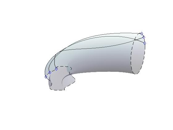
Figure 1. Projected matrix mapping cylinder corresponding to the path $\mathbf{U}_{[0,\frac{1}{2}]}(\hat{u}_{3})$ in $M_{3}$.

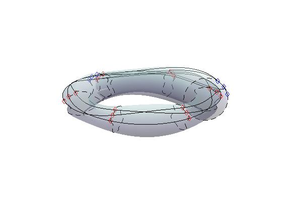
Figure 2. Projected matrix mapping cylinder corresponding to the path $\mathbf{U}_{\mathbb{I}}(\hat{u}_{3})$ in $M_{3}$.

Figure 3. Embedded matrix mapping cylinder corresponding to the path $\mathbf{U}_{\mathbb{I}}(\hat{u}_{3})$ in $M_{3}$.

Alternative methods to trace particular flow lines on mapping cylinders can be otained using matrix homotopies, this can be done using similar methods to the ones implemented in [7].

3.3. Environment algebras

Definition 3.10 (Environment algebra (of a matrix algebra)).

Given a mat-rix algebra $A$ $\subseteq M_{n}$, a universal C^∗-algebra $\mathcal{E}_{A}:=C^{*}_{1}\braket{x_{1},\ldots,x_{m}}{\mathcal{R}(x_{1},\ldots,x_{m})}$ for which there is a matrix representation $\mathcal{E}_{A}\twoheadrightarrow\mathbf{E}_{A}\subseteq M_{n}$ such that $A\subseteq\mathbf{E}_{A}$, will be called an environment algebra for $A$.

Let us consider the universal C^∗-algebras $C(\mathbb{J})$, $C({\mathbb{T}^{1}})$, $C({\mathbb{T}^{1}})\ast_{\mathbb{C}}C({\mathbb{T}^{1}})$, $C_{\delta}({\mathbb{T}^{2}})$, $C_{\delta}(\mathbb{J}\times{\mathbb{T}^{1}})$ and $C^{*}_{\varepsilon}\langle\mathbb{Z}/2\times\mathbb{Z}\rangle$, defined in terms of generators and relations by the expressions.

$$C(\mathbb{J}):=C^{*}_{1}\left\langle u\left|\begin{array}[]{l}h^{*}=h,\|h\|\leq 1\end{array}\right.\right\rangle$$

$$C({\mathbb{T}^{1}}):=C^{*}_{1}\left\langle u\left|\begin{array}[]{l}uu^{*}=u^{*}u=1\end{array}\right.\right\rangle$$

$$C({\mathbb{T}^{1}})\ast_{\mathbb{C}}C({\mathbb{T}^{1}}):=C^{*}_{1}\left\langle u,v\left|\begin{array}[]{l}uu^{*}=u^{*}u=1,\\ vv^{*}=v^{*}v=1\end{array}\right.\right\rangle$$

$$C_{\delta}({\mathbb{T}^{2}}):=C^{*}_{1}\left\langle u,v\left|\begin{array}[]{l}uu^{*}=u^{*}u=1,\\ vv^{*}=v^{*}v=1,\\ \|uv-vu\|\leq\delta\end{array}\right.\right\rangle$$

$$C_{\delta}(\mathbb{J}\times{\mathbb{T}^{1}}):=C^{*}_{1}\left\langle h,u\left|\begin{array}[]{l}h^{*}=h,\|h\|\leq 1\\ uu^{*}=u^{*}u=1,\\ \|hu-uh\|\leq\delta\end{array}\right.\right\rangle$$

$$C^{*}_{\varepsilon}\langle\mathbb{Z}/2\times\mathbb{Z}\rangle:=C^{*}_{1}\left\langle u,v\left|\begin{array}[]{l}uu^{*}=u^{*}u=u^{2}=1,\\ vv^{*}=v^{*}v=1,\\ \|uv-vu\|\leq\varepsilon\end{array}\right.\right\rangle.$$

Let us consider now a local matrix representation result that we will use later in the construction of particular representation schemes.

Lemma 3.1.

For every integer $n\geq 1$, there are $s_{2},u_{n},v_{n}\in\mathbb{U}(\mathcal{M}_{\infty})$ such that the diagram

commutes, where $s_{2}\in\mathbb{H}(n)$, $u_{n}$ and $v_{n}$ are unitary elements in $M_{n}$.

Proof.

Since we have that $C({\mathbb{T}^{1}})^{\ast 2}\simeq C^{*}\braket{\mathbb{F}_{2}}\simeq C^{*}(\mathbb{Z}^{\ast 2})$, by universality of the C^∗-representa-tions

$$C^{*}(\mathbb{Z}^{\ast 2}) \simeq C^{*}\left\langle u,v\left|\begin{array}[]{l}uu^{*}=u^{*}u=\mathbb{1},\\ vv^{*}=v^{*}v=\mathbb{1}\end{array}\right.\right\rangle$$

$$C^{*}((\mathbb{Z}/n)^{\ast 2}) \simeq C^{*}\left\langle u,v\left|\begin{array}[]{l}uu^{*}=u^{*}u=\mathbb{1},\\ vv^{*}=v^{*}v=\mathbb{1},\\ u^{n}=v^{n}=\mathbb{1}\end{array}\right.\right\rangle$$

$$C^{*}(\mathbb{Z}/n\ast\mathbb{Z}/2) \simeq C^{*}\left\langle u,v\left|\begin{array}[]{l}uu^{*}=u^{*}u=\mathbb{1},\\ vv^{*}=v^{*}v=\mathbb{1},\\ u^{n}=v^{2}=\mathbb{1}\end{array}\right.\right\rangle,$$

and by the structural properties of $M_{n}$, it is enough to find for any $n\in\mathbb{Z}^{+}$, up to unitary congruence in $M_{n}$, three unitaries $s_{2},u_{n},v_{n}\in\mathbb{U}(n)$ such that $C^{*}(s_{2},v_{n})=M_{n}=C^{*}(u_{n},v_{n})$ and $u_{n}^{n}=v_{n}^{n}=s_{2}^{2}=\mathbb{1}_{n}$, this can be done by taking for any $n\in\mathbb{Z}^{+}$ the orthogonal projection $p:=\mathrm{diag}\left[1,0,\ldots,0\right]\in\mathbb{H}(n)$ and the matrix $s_{2}=\mathbb{1}-2p\in\mathbb{H}(n)$, setting $u_{n}:=\Omega_{n}$ and $v_{n}:=\Sigma_{n}$ for $n\geq 2$ and $u_{1}=v_{1}=1$ for $n=1$, by functional calculus and direct computations it is easy to verify that $s_{2},u_{n},v_{n}\in\mathbb{U}(n)$ for every $n\in\mathbb{Z}^{+}$, and that $s_{2}=s_{2}^{*}$, it is also easy to verify that the system of matrix units $\set{e_{i,j,n}}_{1\leq i,j\leq n}$ and $u_{n}$ can be expressed as words in $C^{*}(s_{2},v_{n})$ for every $n\in\mathbb{Z}^{+}$, it is also clear that $p=e_{1,1,n}$ and hence, $s_{2}$ can be written as linear combinations of words in $C^{*}(u_{n},v_{n})$, we will then have that $C^{*}\braket{\mathbb{Z}/n\ast\mathbb{Z}/2}\twoheadrightarrow C^{*}(v_{n},s_{2})$ and $C^{*}\braket{\mathbb{Z}/n^{\ast 2}}\twoheadrightarrow C^{*}(u_{n},v_{n})$ by the universal properties of $C^{*}\braket{\mathbb{Z}/2\ast\mathbb{Z}/n}$ and $C^{*}\braket{\mathbb{Z}/n^{\ast 2}}$ respectively, since it can be easily verified that

$$u_{n}^{n}=v_{n}^{n}=s_{2}^{2}=\mathbb{1}_{n},$$

from these facts and the universal property of $C({\mathbb{T}^{1}})^{\ast 2}\simeq C^{*}\braket{\mathbb{F}_{2}}\simeq C^{*}\braket{\mathbb{Z}^{\ast 2}}$, the result follows. ∎

Remark 3.3.

It can be seen that for any matrix C^∗-subalgebra $A\subseteq M_{n}$, there is $\delta>0$ such that both $C({\mathbb{T}^{1}})\ast_{\mathbb{C}}C({\mathbb{T}^{1}})$ and $C_{\delta}({\mathbb{T}^{2}})$ are environment algebras of $A$. It can also be seen that for any abelian C^∗-subalgebra $D\subseteq M_{n}$, $C({\mathbb{T}^{1}})$ is an environment algebra of $D$.

4. Local Matrix Connectivity

4.1. Topologically controlled linear algebra and Soft Tori

Definition 4.1 (Controlled sets of matrix functions).

Given $\delta>0$, a function $\varepsilon:\mathbb{R}\to\mathbb{R}^{+}_{0}$, a finite set of functions $F\subseteq C({\mathbb{T}^{1}},{\mathbb{D}^{2}})$ and two unitary matrices $u,v\in M_{n}$ such that $\|uv-vu\|\leq\delta$, we say that the set $F$ is $\delta$-controlled by $\mathrm{Ad}[v]$ if the diagram,

commutes up to an error $\varepsilon(\delta)$ for each $f\in F$.

Remark 4.1.

The $C^{*}$-homomorphism $C_{\delta}({\mathbb{T}^{2}})\to C^{*}(u,v)$ allows us to see that the Soft Torus $C_{\delta}({\mathbb{T}^{2}})$ provides an environment algebra for any $\delta$-controlled set of matrix functions.

Lemma 4.1 (Existence of isospectral approximants).

Given $\varepsilon>0$ there is $\delta>0$ such that, for any $2$ families of $N$ pairwise commuting normal matrices $x_{1},\ldots,x_{N}$ and $y_{1},\ldots,y_{N}$ which satisfy the constraints $\|x_{j}-y_{j}\|\leq\delta$ for each $1\leq j\leq N$, there is a $C^{*}$-homomorphism $\Psi$ such that $\sigma(\Psi(x_{j}))=\sigma(x_{j})$, $[\Psi(x_{j}),y_{j}]=0$ and $\max\{\|\Psi(x_{j})-y_{j}\|,\|\Psi(x_{j})-x_{j}\|\}\leq\varepsilon$, for each $1\leq j\leq N$.

Proof.

By changing basis if necessary, we can assume that $y_{1},\ldots,y_{N}$ are diagonal matrices. From T.2.1 we will have that there is a permutation $\tau$ of the index set $\{1,\ldots,n\}$ such that for each $1\leq k\leq n$ we have that

(4.1) $$|\Lambda^{(k)}(x_{j})-\Lambda^{(\tau(k))}(y_{j})| \leq \|\Lambda^{(k)}(x_{1},\ldots,x_{N})-\Lambda^{(\tau(k))}(y_{1},\ldots,y_{N})\|$$

$$\leq e_{N,0}\|\mathrm{Cliff}(x_{1}-y_{1},\ldots,x_{N}-y_{N})\|.$$

Using 2.9 and as a consequence of 4.1 we can find a permutation matrix $\mathcal{T}\in\mathbb{U}(n)$ such that

(4.2) $$\|\mathcal{T}^{*}\mathrm{diag}\left[\Lambda(x_{j})\right]\mathcal{T}-\mathrm{diag}\left[\Lambda(y_{j})\right]\| \leq e_{N,0}\|\mathrm{Cliff}(x_{1}-y_{1},\ldots,x_{N}-y_{N})\|$$

$$\leq e_{N,0}N\delta,\>\>1\leq j\leq N.$$

Let us set $c_{N}:=e_{N,0}N$. For the matrices $x_{1},\ldots,x_{N}$ there is a unitary joint diagonalizer $W\in M_{n}$ such that $W\mathrm{diag}\left[\Lambda(x_{j})\right]W^{*}=x_{j}$, $1\leq j\leq N$,

(4.3) $$\|W\mathrm{diag}\left[\Lambda(x_{j})\right]W^{*}-\mathcal{T}^{*}\mathrm{diag}\left[\Lambda(x_{j})\right]\mathcal{T}\| \leq \|W\mathrm{diag}\left[\Lambda(x_{j})\right]W^{*}-y_{j}\|$$

$$+\|y_{j}-\mathcal{T}^{*}\mathrm{diag}\left[\Lambda(x_{j})\right]\mathcal{T}\|$$

$$\leq (1+c_{N})\|x_{j}-y_{j}\|\leq(1+c_{N})\delta.$$

If we set $V:=W\mathcal{T}$ and $\varepsilon=(1+c_{N})\delta$, we will have that by 4.2 and 4.3 the inner $C^{*}$-automorphism $\Psi:=\mathrm{Ad}[V^{*}]$ satisfies the constraints in the statement of this lemma, and we are done. ∎

Remark 4.2.

The $C^{*}$-automorphism $\Psi$ from L.4.1 is called an isospectral approximant for the two $N$-tuples $x_{1},\ldots,x_{N}$ and $y_{1},\ldots,y_{N}$. If $\Psi:=\mathrm{Ad}[W^{*}]$ for some $W\in\mathbb{U}(n)$, then we will have that its inverse $\Psi^{\dagger}$ will be given by the expression $\Psi^{\dagger}=\mathrm{Ad}[W]$.

Remark 4.3.

The constant $c_{N}$ in the proof of L.4.1 depends only on the number $N$ of matrices in each family. It does not depend on the matrix size.

4.2. Local piecewise analytic connectivity

In this section we will present some piecewise analytic local connectivity results in matrix representations of the form $C_{\varepsilon}({\mathbb{T}^{2}})\to M_{n}\leftarrow C({\mathbb{T}^{N}})$ and $C_{\varepsilon}(\mathbb{J}\times{\mathbb{T}^{1}})\to M_{n}\leftarrow C(\mathbb{J}^{N})$.

Theorem 4.1 (Local normal toral connectivity).

Given $\varepsilon>0$ and any $n\in\mathbb{Z}^{+}$, there is $\delta>0$ such that, for any $2N$ normal contractions $x_{1},\ldots,x_{N}$ and $y_{1},\ldots,$ $y_{N}$ in $M_{n}$ which satisfy the relations

$$\left\{\begin{array}[]{l}[x_{j},x_{k}]=[y_{j},y_{k}]=0,\>\>\>1\leq j,k\leq N,\\ \|x_{j}-y_{j}\|\leq\delta,\>\>\>1\leq j\leq N,\end{array}\right.$$

there exist $N$ toral matrix links $X^{1},\ldots,X^{N}$ in $M_{n}$, which solve the problems

$$x_{j}\rightsquigarrow y_{j},\>\>\>1\leq j\leq N,$$

and satisfy the constraints

$$\left\{\begin{array}[]{l}\|X_{t}^{j}(x_{j})-y_{j}\|\leq\varepsilon,\end{array}\right.$$

for each $1\leq j,k\leq N$ and each $t\in\mathbb{I}$. Moreover, $\ell_{\|\cdot\|}(X_{t}^{j}(x_{j}))\leq\varepsilon,\>\>\>1\leq j\leq N$.

Proof.

By L.2.1, L.2.2 and L.4.1 we will have that given $\varepsilon>0$, there are $0<\delta\leq\nu\leq\varepsilon/2$ and an isospectral approximant $\Psi:=\mathrm{Ad}[W^{*}]$ (with $W\in\mathbb{U}(n)$) for $x_{1},\ldots,x_{N}$ and $y_{1},\ldots,y_{N}$ such that, $\max\{\|x_{j}-\Psi(x_{j})\|,\|y_{j}-\Psi(x_{j})\|\}\leq\nu$ and $[\Psi(x_{j}),y_{j}]=0$ for each $1\leq j\leq N$, we will also have that there is a unitary path $\mathcal{W}\in C(\mathbb{I},M_{n})$ which is defined by the expression $\mathcal{W}_{t}:=e^{-itH_{W}}$ for each $t\in\mathbb{I}$, where $H_{W}\in M_{n}$ is a hermitian matrix such that $e^{iH_{W}}=W$ and $\|[H_{W},x_{j}]\|\leq\varepsilon/2$ for each $1\leq j\leq N$, and that is defined by $H_{W}:=h(W)$, for some function $h:\Omega^{\alpha}_{d,s}\rightarrow[-1,1]$, and where $\sigma(W)\subset\Omega^{\alpha}_{d,s}:=\{e^{i(\pi t+\alpha)}|-1+s<t<1-s\}\subset{\mathbb{T}^{1}}$, with $s,\alpha\in\mathbb{R}$ chosen in such a way that ${\mathbb{T}^{1}}\backslash\Omega^{\alpha}_{d,s}$ contains an arc of length $d$ (with $d\geq 2\pi/n$). Moreover, we can choose $\delta$ and $\nu$ in such a way that the path $\mathcal{W}$ satisfies the inequalities $\|[\mathcal{W}_{t},\Psi(x_{j})]\|\leq\varepsilon/2$ for each $t\in[0,1]$ and each $1\leq j\leq N$.

It can be seen that the paths $\breve{X}^{j}_{t}:=\mathrm{Ad}[\mathcal{W}_{t}](x_{j})$ will solve the problem $x_{j}\rightsquigarrow_{\varepsilon/2}\Psi(x_{j})$ for each $1\leq j\leq N$. Let us set $\bar{X}_{t}^{j}:=(1-t)\Psi(x_{j})+ty_{j}$, we can now construct $N$ toroidal matrix links of the form $X^{j}:=\breve{X}^{j}\circledast\bar{X}^{j}$ which solve the problems $x_{j}\rightsquigarrow y_{j}$, locally preserve normality and commutativity and satisfy the $\|\cdot\|$-distance constraints

$$\|X^{j}_{t}-y_{j}\| \leq \|X^{j}_{t}-\Psi({x}_{j})\|+\|y_{j}-\Psi({x}_{j})\|$$

$$\leq \frac{\varepsilon}{2}+\nu$$

$$\leq \frac{\varepsilon}{2}+\frac{\varepsilon}{2}=\varepsilon,$$

together with the $\|\cdot\|$-length constraints

(4.4) $$\ell_{\|\cdot\|}(X^{j}_{t}) \leq \ell_{\|\cdot\|}(\breve{X}^{j}_{t})+\|\Psi({x}_{j})-y_{j}\|$$

(4.5) $$= \int_{\mathbb{I}}\|\partial_{t}\mathrm{Ad}[\mathcal{W}_{t}](x_{j})\|dt+\|\Psi({x}_{j})-y_{j}\|$$

(4.6) $$= \|[H_{W},\Psi({x}_{j})]\|+\|\Psi({x}_{j})-y_{j}\|$$

(4.7) $$\leq \frac{\varepsilon}{2}+\nu\leq\varepsilon,$$

which hold whenever $\|x_{j}-y_{j}\|\leq\delta$, $1\leq j\leq N$, and we are done. ∎

Remark 4.4.

It can be noticed that the solvent matrix links $X^{1},\ldots$ $,X^{N}$ whose existence is stated in T.4.1 are factored in the form $X^{j}=\breve{X}^{j}\circledast\bar{X}^{j}$, we call $\breve{X}^{j}$ and $\bar{X}^{j}$ the curved and flat factors of $X^{j}$ respectively.

We will derive now, some corollaries of the proof of T.4.1.

Corollary 4.1 (Local hermitian toral connectivity).

Given $\varepsilon>0$ and any integer $n\geq 1$, there is $\delta>0$ such that, for any $2N$ hermitian contractions $x_{1},\ldots,x_{N}$ and $y_{1},\ldots,y_{N}$ in $M_{n}$ which satisfy the relations

$$\left\{\begin{array}[]{l}[x_{j},x_{k}]=[y_{j},y_{k}]=0,\>\>\>1\leq j,k\leq N,\\ \|x_{j}-y_{j}\|\leq\delta,\>\>\>1\leq j\leq N,\end{array}\right.$$

there exist $N$ toral matrix links $X^{1},\ldots,X^{N}$ in $M_{n}$, which solve the problems

$$x_{j}\rightsquigarrow y_{j},\>\>\>1\leq j\leq N,$$

and satisfy the constraints

$$\left\{\begin{array}[]{l}X_{t}^{j}(x_{j})=(X_{t}^{j}(x_{j}))^{*},\\ \|X_{t}^{j}(x_{j})-y_{j}\|\leq\varepsilon,\end{array}\right.$$

for each $1\leq j,k\leq N$ and each $t\in\mathbb{I}$. Moreover, $\ell_{\|\cdot\|}(X_{t}^{j}(x_{j}))\leq\varepsilon,\>\>\>1\leq j\leq N$.

Proof.

Since for any $\alpha\in\mathbb{R}$, any pair of hermitian matrices $x,y\in\mathbb{H}(n)$ and any partial unitary $z\in\mathbb{PU}(n)$, we have that $x+\alpha(y-x)$ and $zxz^{*}$ are also in $\mathbb{H}(n)$, the result follows as a consequence of L.4.1 and T.4.1. ∎

Corollary 4.2 (Local unitary toral connectivity).

Given any $\varepsilon\geq 0$ and any integer $n\geq 1$, there is $\delta\geq 0$ such that given any $2N$ unitary matrices $U_{1},\ldots,U_{N}$ ,$V_{1},\ldots,V_{N}$ in $M_{n}$ which satisfy the relations

$$\left\{\begin{array}[]{l}[U_{j},U_{k}]=[V_{j},V_{k}]=0,\\ \|U_{k}-V_{k}\|\leq\delta,\end{array}\right.$$

for each $1\leq j,k\leq N$, there are toral matrix links $u^{1},\ldots,u^{N}$ in $M_{n}$ which solve the interpolation problems

$$U_{k}\rightsquigarrow V_{k},\>\>\>1\leq k\leq N,$$

and also satisfy the relations

$$\left\{\begin{array}[]{l}(u^{j}_{t})^{*}u^{j}_{t}=u^{j}_{t}(u^{j}_{t})^{*}=\mathbb{1}_{n},\\ \|u^{j}_{t}-V_{j}\|\leq\varepsilon,\end{array}\right.$$

for each $t\in\mathbb{I}$ and each $1\leq j,k\leq N$. Moreover, $\ell_{\|\cdot\|}(u^{j}_{t})\leq\varepsilon$, $1\leq j\leq N$.

Proof.

Since for any $C^{*}$-automorphisms $\Psi$ we have that $\Psi(\mathbb{U}(n))\subseteq\mathbb{U}(n)$, and since any two commuting unitaries $U$ and $V$ can connected by a flat unitary path $\bar{U}_{t}:=Ue^{t\ln\left(U^{*}V\right)}$, for $0\leq t\leq 0$. We will have that the result can be derived using a similar argument to the one implemented in the proof of T.4.1. ∎

4.2.1. Lifted local piecewise analytic connectivity

Let us denote by $\kappa$ the matrix compression $M_{2n}\to M_{n}$ defined by the mapping

$$\kappa:M_{2n}\to M_{n},\left(\begin{array}[]{cc}x_{11}&x_{12}\\ x_{21}&x_{22}\end{array}\right)\mapsto x_{11}.$$

Let us write $\imath_{2}:M_{n}\to M_{2n}$ to denote the $C^{*}$-homomorphism defined by the expression $\imath_{2}(x):=x\oplus x=\mathbb{1}_{2}\otimes x$.

Definition 4.2 (Standard dilations).

Given a $C^{*}$-automorphism $\Psi:=\mathrm{Ad}[W]$ (with $W\in\mathbb{U}(n)$) in $M_{n}$, we will denote by $\Psi^{[s]}$ the $C^{*}$-automorphism in $M_{2n}$ defined by the expression $\Psi^{[s]}:=\mathrm{Ad}[\mathbb{1}_{2}\otimes W]=\mathrm{Ad}[W\oplus W]$. We call $\Psi^{[s]}$ a standard dilation of $\Psi$.

Definition 4.3 ($\mathbb{Z}/2$-dilations).

Given a $C^{*}$-automorphism $\Psi:=\mathrm{Ad}[W]$ (with $W\in\mathbb{U}(n)$) in $M_{n}$, we will denote by $\Psi^{[2]}$ the $C^{*}$-automorphism in $M_{2n}$ defined by the expression $\Psi^{[2]}:=\mathrm{Ad}[(\Sigma_{2}\otimes\mathbb{1}_{n})(W^{*}\oplus W)]$. We call $\Psi^{[2]}$ a $\mathbb{Z}/2$-dilation of $\Psi$.

Remark 4.5.

It can be seen that $\kappa(\imath_{2}(x))=x$ for any $x\in M_{2n}$, it can also be seen that $\kappa(\Psi^{[2]}(\imath_{2}(x)))=\kappa(\Psi^{[s]}(\imath_{2}(x)))$.

Theorem 4.2 (Lifted local toral connectivity).

Given $\varepsilon>0$, there is $\delta>0$ such that, for any $2N$ normal contractions $x_{1},\ldots,x_{N}$ and $y_{1},\ldots,y_{N}$ in $M_{n}$ which satisfy the relations

$$\left\{\begin{array}[]{l}[x_{j},x_{k}]=[y_{j},y_{k}]=0,\>\>\>1\leq j,k\leq N,\\ \|x_{j}-y_{j}\|\leq\delta,\>\>\>1\leq j\leq N,\end{array}\right.$$

there is a $C^{*}$-homomorphism $\Phi:M_{n}\to M_{2n}$ and $N$ toral matrix links $X^{1},\ldots,$ $X^{N}$ in $C(\mathbb{I},M_{2n})$, which solve the problems

$$\Phi(x_{j})\rightsquigarrow y_{j}\oplus y_{j},\>\>\>1\leq j\leq N,$$

and satisfy the constraints

$$\left\{\begin{array}[]{l}\kappa(\Phi(x_{j}))=x_{j},\\ \|\Phi(x_{j})-x_{j}\oplus x_{j}\|\leq\varepsilon,\\ \|X_{t}^{j}-y_{j}\oplus y_{j}\|\leq\varepsilon,\end{array}\right.$$

for each $1\leq j,k\leq N$ and each $t\in\mathbb{I}$. Moreover, $\ell_{\|\cdot\|}(X_{t}^{j})\leq\varepsilon,\>\>\>1\leq j\leq N$.

Proof.

By L.4.1 we will have that given $\varepsilon>0$, there are $0<\delta\leq\nu=\frac{\varepsilon}{2\pi}$ and an isospectral approximant $\Psi:=\mathrm{Ad}[W^{*}]$ (with $W\in\mathbb{U}(n)$) for $x_{1},\ldots,x_{N}$ and $y_{1},\ldots,y_{N}$ such that, $\max\{\|x_{j}-\Psi(x_{j})\|,\|y_{j}-\Psi(x_{j})\|\}\leq\nu$. By setting $\Phi:=(\Psi^{\dagger})^{[2]}\circ\imath_{2}\circ\Psi$, by D.4.3, D.4.2 and R.4.5 it can be seen that $\Phi:M_{n}\to M_{2n}$ is a $C^{*}$-homomorphism such that $\|\Phi(x_{j})-\imath_{2}(x_{j})\|=\|\Phi(x_{j})-x_{j}\oplus x_{j}\|\leq\varepsilon$, for each $1\leq j\leq N$.

Since $(\Psi^{\dagger})^{[2]}:=\mathrm{Ad}[\hat{W}_{s}]$ with $\hat{W}_{s}:=(\Sigma_{2}\otimes\mathbb{1}_{n})(W^{*}\oplus W)$ and since $\hat{W}_{s}\in\mathbb{U}(2n)\cap\mathbb{H}(2n)$, we will have that $\hat{W}_{s}$ can be represented as $\hat{W}_{s}=e^{i\frac{\pi}{2}(\hat{W}_{s}-\mathbb{1}_{2n})}$ for any $n\geq 1$. If we set $\tilde{X}_{j}:=\Psi^{[s]}(\imath_{2}({x}_{j}))$, $1\leq j\leq N$, we also have that there is a unitary path $\{\mathcal{W}_{t}\}_{t\in\mathbb{I}}\subset M_{2n}$ with $\mathcal{W}_{t}:=e^{i\frac{\pi(1-t)}{2}(\hat{W}_{s}-\mathbb{1}_{2n})}$, which satisfies the conditions $\mathcal{W}_{0}=\hat{W}_{s}$, $\mathcal{W}_{1}=\mathbb{1}_{2n}$, together with the normed estimates

$$\|\mathcal{W}_{t}\tilde{X}_{j}-\tilde{X}_{j}\mathcal{W}_{t}\| = |\cos(\pi t/2)|\|\hat{W}_{s}\tilde{X}_{j}-\tilde{X}_{j}\hat{W}_{s}\|$$

$$\leq \|\hat{W}_{s}\tilde{X}_{j}-\tilde{X}_{j}\hat{W}_{s}\|\leq\nu,$$

for each $1\leq j\leq N$ and each $0\leq t\leq 1$. Moreover, for each $1\leq j\leq N$ we have that the paths $\breve{X}^{j}_{t}:=\mathrm{Ad}[\mathcal{W}_{t}](\tilde{X}_{j})$ satisfy the normed estimates

$$\ell_{\|\cdot\|}(\breve{X}_{t}^{j}) = \int_{\mathbb{I}}\|\partial_{t}\mathrm{Ad}[\mathcal{W}_{t}](\tilde{X}_{j}))\|dt,$$

$$= \frac{\pi}{2}\|\hat{W}_{s}\tilde{X}_{j}-\tilde{X}_{j}\hat{W}_{s}\|\leq\nu.$$

For each $1\leq j\leq N$, we can now use the flat paths $\bar{X}_{t}^{j}:=(1-t)\tilde{X}_{j}+t\imath_{2}(y_{j})$ together with the previously described curved paths $\breve{X}^{j}$ to construct the solvent toral matrix links $X^{1},\ldots,X^{N}\in C([0,1],M_{2n})$ we are looking for, and which can be defined by $X^{j}:=\breve{X}^{j}\circledast\bar{X}^{j}$ for each $1\leq j\leq N$, and we are done. ∎

Remark 4.6.

It can be seen that by using the technique implemented in the proof of T.4.2 one can obtain lifted versions of C.4.2 and C.4.1.

Remark 4.7.

As a consequence of T.4.2 we can derive simple detection methods to identify families of pairwise commuting matrices in $M_{n}$ that can be connected uniformly via piecewise analytic toral matrix links. The existence of these detection methods raises some interesting questions for further studies.

Remark 4.8.

We can interpret T.4.2 as an existence theorem of solutions to lifted connectivity problems defined on matrix representations of the form

$$\lx@xy@svg{\hbox{\raise 0.0pt\hbox{\kern 16.88405pt\hbox{\ignorespaces\ignorespaces\ignorespaces\hbox{\vtop{\kern 0.0pt\offinterlineskip\halign{\entry@#!@&&\entry@@#!@\cr&&&\\&&&\crcr}}}\ignorespaces{\hbox{\kern-3.0pt\raise 0.0pt\hbox{\hbox{\kern 0.0pt\raise 0.0pt\hbox{\hbox{\kern 3.0pt\raise 0.0pt\hbox{$\textstyle{}$}}}}}}}{\hbox{\kern 40.88405pt\raise 0.0pt\hbox{\hbox{\kern 0.0pt\raise 0.0pt\hbox{\hbox{\kern 3.0pt\raise 0.0pt\hbox{$\textstyle{C_{\varepsilon}^{*}\langle\mathbb{Z}/2\times\mathbb{Z}\rangle\ignorespaces\ignorespaces\ignorespaces\ignorespaces}$}}}}}}}\ignorespaces\ignorespaces\ignorespaces\ignorespaces{}{\hbox{\lx@xy@droprule}}\ignorespaces{\hbox{\kern 124.97656pt\raise 0.0pt\hbox{\hbox{\kern 0.0pt\raise 0.0pt\hbox{\lx@xy@tip{1}\lx@xy@tip{-1}}}}}}{\hbox{\lx@xy@droprule}}{\hbox{\lx@xy@droprule}}{\hbox{\kern 124.97656pt\raise 0.0pt\hbox{\hbox{\kern 0.0pt\raise 0.0pt\hbox{\hbox{\kern 3.0pt\raise 0.0pt\hbox{$\textstyle{C^{*}(\hat{U}_{s},\hat{V})\ignorespaces\ignorespaces\ignorespaces\ignorespaces}$}}}}}}}\ignorespaces\ignorespaces\ignorespaces\ignorespaces{}{\hbox{\lx@xy@droprule}}\ignorespaces{\hbox{\kern 191.32726pt\raise 0.0pt\hbox{\hbox{\kern 0.0pt\raise 0.0pt\hbox{\lx@xy@tip{1}\lx@xy@tip{-1}}}}}}{\hbox{\lx@xy@droprule}}{\hbox{\lx@xy@droprule}}{\hbox{\kern 191.32726pt\raise 0.0pt\hbox{\hbox{\kern 0.0pt\raise 0.0pt\hbox{\hbox{\kern 3.0pt\raise 0.0pt\hbox{$\textstyle{M_{2n}\ignorespaces\ignorespaces\ignorespaces\ignorespaces}$}}}}}}}\ignorespaces\ignorespaces\ignorespaces\ignorespaces{}{\hbox{\lx@xy@droprule}}\ignorespaces{\hbox{\kern 202.80374pt\raise-31.0536pt\hbox{\hbox{\kern 0.0pt\raise 0.0pt\hbox{\lx@xy@tip{1}\lx@xy@tip{-1}}}}}}{\hbox{\lx@xy@droprule}}{\hbox{\lx@xy@droprule}}{\hbox{\kern-16.88405pt\raise-40.88692pt\hbox{\hbox{\kern 0.0pt\raise 0.0pt\hbox{\hbox{\kern 3.0pt\raise 0.0pt\hbox{$\textstyle{C^{*}\langle\mathbb{F}_{2}\rangle\ignorespaces\ignorespaces\ignorespaces\ignorespaces\ignorespaces\ignorespaces\ignorespaces\ignorespaces}$}}}}}}}\ignorespaces\ignorespaces\ignorespaces\ignorespaces{}{\hbox{\lx@xy@droprule}}\ignorespaces{\hbox{\kern 53.15637pt\raise-40.88692pt\hbox{\hbox{\kern 0.0pt\raise 0.0pt\hbox{\lx@xy@tip{1}\lx@xy@tip{-1}}}}}}{\hbox{\lx@xy@droprule}}{\hbox{\lx@xy@droprule}}\ignorespaces\ignorespaces\ignorespaces{}\ignorespaces\ignorespaces{\hbox{\lx@xy@drawline@}}\ignorespaces{\hbox{\kern 60.78432pt\raise-5.5pt\hbox{\hbox{\kern 0.0pt\raise 0.0pt\hbox{\lx@xy@tip{1}\lx@xy@tip{-1}}}}}}\ignorespaces\ignorespaces{\hbox{\lx@xy@drawline@}}\ignorespaces{\hbox{\lx@xy@drawline@}}{\hbox{\kern 53.15637pt\raise-40.88692pt\hbox{\hbox{\kern 0.0pt\raise 0.0pt\hbox{\hbox{\kern 3.0pt\raise 0.0pt\hbox{$\textstyle{C_{\delta}(\mathbb{T}^{2})\ignorespaces\ignorespaces\ignorespaces\ignorespaces}$}}}}}}}\ignorespaces\ignorespaces\ignorespaces\ignorespaces{}{\hbox{\lx@xy@droprule}}\ignorespaces{\hbox{\kern 123.5801pt\raise-40.88692pt\hbox{\hbox{\kern 0.0pt\raise 0.0pt\hbox{\lx@xy@tip{1}\lx@xy@tip{-1}}}}}}{\hbox{\lx@xy@droprule}}{\hbox{\lx@xy@droprule}}{\hbox{\kern 123.5801pt\raise-40.88692pt\hbox{\hbox{\kern 0.0pt\raise 0.0pt\hbox{\hbox{\kern 3.0pt\raise 0.0pt\hbox{$\textstyle{C^{*}(U,V)\ignorespaces\ignorespaces\ignorespaces\ignorespaces\ignorespaces\ignorespaces\ignorespaces\ignorespaces}$}}}}}}}\ignorespaces\ignorespaces\ignorespaces\ignorespaces{}{\hbox{\lx@xy@droprule}}\ignorespaces{\hbox{\kern 145.45367pt\raise-5.5pt\hbox{\hbox{\kern 0.0pt\raise 0.0pt\hbox{\lx@xy@tip{1}\lx@xy@tip{-1}}}}}}{\hbox{\lx@xy@droprule}}{\hbox{\lx@xy@droprule}}\ignorespaces\ignorespaces\ignorespaces\ignorespaces{}{\hbox{\lx@xy@droprule}}\ignorespaces{\hbox{\kern 192.72726pt\raise-40.88692pt\hbox{\hbox{\kern 0.0pt\raise 0.0pt\hbox{\lx@xy@tip{1}\lx@xy@tip{-1}}}}}}{\hbox{\lx@xy@droprule}}{\hbox{\lx@xy@droprule}}{\hbox{\kern 192.72726pt\raise-40.88692pt\hbox{\hbox{\kern 0.0pt\raise 0.0pt\hbox{\hbox{\kern 3.0pt\raise 0.0pt\hbox{$\textstyle{M_{n}}$}}}}}}}\ignorespaces}}}}\ignorespaces, \textstyle{C_{\varepsilon}^{*}\langle\mathbb{Z}/2\times\mathbb{Z}\rangle\ignorespaces\ignorespaces\ignorespaces\ignorespaces} \textstyle{C^{*}(\hat{U}_{s},\hat{V})\ignorespaces\ignorespaces\ignorespaces\ignorespaces} \textstyle{M_{2n}\ignorespaces\ignorespaces\ignorespaces\ignorespaces} \textstyle{C^{*}\langle\mathbb{F}_{2}\rangle\ignorespaces\ignorespaces\ignorespaces\ignorespaces\ignorespaces\ignorespaces\ignorespaces\ignorespaces} \textstyle{C_{\delta}(\mathbb{T}^{2})\ignorespaces\ignorespaces\ignorespaces\ignorespaces} \textstyle{C^{*}(U,V)\ignorespaces\ignorespaces\ignorespaces\ignorespaces\ignorespaces\ignorespaces\ignorespaces\ignorespaces} \textstyle{M_{n}} \textstyle{C_{\varepsilon}^{*}\langle\mathbb{Z}/2\times\mathbb{Z}\rangle\ignorespaces\ignorespaces\ignorespaces\ignorespaces} \textstyle{C^{*}(\hat{U}_{s},\hat{V})\ignorespaces\ignorespaces\ignorespaces\ignorespaces} \textstyle{M_{2n}\ignorespaces\ignorespaces\ignorespaces\ignorespaces} \textstyle{C^{*}\langle\mathbb{F}_{2}\rangle\ignorespaces\ignorespaces\ignorespaces\ignorespaces\ignorespaces\ignorespaces\ignorespaces\ignorespaces} \textstyle{C_{\delta}(\mathbb{T}^{2})\ignorespaces\ignorespaces\ignorespaces\ignorespaces} \textstyle{C^{*}(U,V)\ignorespaces\ignorespaces\ignorespaces\ignorespaces\ignorespaces\ignorespaces\ignorespaces\ignorespaces} \textstyle{M_{n}}$$

with $\hat{U}_{s}=(\Sigma_{2}\otimes\mathbb{1}_{n})(U^{*}\oplus U)$ and $\hat{V}=V\oplus V$.

Some further applications of T.4.2 to approximation of matrix words and norm behavior will be presented in [33].

4.2.2. Matrix Klein Bottles: Local matrix deformations and special symmetries

Using T.4.2 we can solve all connectivity problems (together with their softened versions) in $M_{n}$ that can be reduced to connectiviy problems of the form $x\rightsquigarrow_{\varepsilon}x^{*}$ in $\mathcal{N}(n)({\mathbb{D}^{2}})$, with $x^{*}=TxT$ and $T^{2}=\mathbb{1}_{n}$.

Remark 4.9.

For each $\varepsilon\in[0,2]$, we can use the previously described symmetries and $\mathscr{D}_{\mathbb{T}}$ to interpret $\bigcup_{x\in M_{n}}\{x\rightsquigarrow_{\varepsilon}x^{*}\}$ as matrix analogies of the Klein bottle.

By a softened matrix Klein bottle we mean that the symmetries are softened, in particular we can consider the connectiviy problems $x\rightsquigarrow_{\varepsilon}x^{*}$ and $y\rightsquigarrow_{\varepsilon}y^{*}$ in $\mathcal{N}(n)({\mathbb{D}^{2}})$ subject to the normed constraints $\|xy-yx\|\leq\delta$, $\|x^{*}-TxT\|,\|xT-Ty\|\leq\delta$ and $T^{2}=\mathbb{1}_{n}$. The details regarding to the solvability of these local connectivity problems will be addressed in future communications.

4.3. $C^{0}$ uniform local connectivity of pairs of unitaries and piecewise analytic approximants

The technique presented in this section can be used to solve local connectivity problems in matrix representations of the form $C_{\varepsilon}({\mathbb{T}^{2}})\to M_{n}\leftarrow C({\mathbb{T}^{2}})$ uniformly via $C^{0}$-unitary paths.

Suppose $U_{t}$ and $V_{t}$ are unitary matrices in $\mathbf{M}_{n}(\mathbb{C})$ for $t=0$ and $t=1$ and we define

(4.11) $$U_{t}=U_{0}e^{t\ln\left(U_{0}^{*}U_{1}\right)}$$

and

(4.12) $$V_{t}=V_{0}e^{t\ln\left(V_{0}^{*}V_{1}\right)}.$$

For $t=0$ or $t=1$ the $C^{*}$-algebra generated by $U_{t}$ and $V_{t}$ is abelian, so select a MASA $C_{t}\cong\mathbb{C}^{n}$ in each case. Let

$$A(C_{0},C_{1})=\left\{\left.X\in C\left([0,1],\mathbf{M}_{n}(\mathbb{C})\right)\right|X(0)\in C_{0}\mbox{ and }X(1)\in C_{1}\right\}.$$

Lemma 4.2.

The $C^{*}$-algebra $A(C_{0},C_{1})$ has stable rank one.

Proof.

Starting with $X$ continuous with $X(t)$ in $C_{t}$ at the endpoints, we can adjust this by a small amount, leaving the endpoints in $C_{t}$, to get $X$ piece-wise linear, with the endpoints of every linear segment having no spectral multiplicity and being invertible. Using Kato’s theory of analytic paths, we can get a piece-wise continuous unitary $U_{t}$ and piece-wise analytic scalar paths $\lambda_{n}(t)$ so that the new path $Y\approx X$ satisfies

$$Y(t)=U_{t}\left[\begin{array}[]{ccc}\lambda_{1}(t)\\ &\ddots\\ &&\lambda_{n}(t)\end{array}\right]U_{t}^{*}.$$

There may be finitely may places where $Y(t)$ is not invertible. These places will be in the interior of the segment so in an open interval where $U_{t}$ is continuous. A small deformation of some of the $\lambda_{j}$ will take the path through invertibles. We have not moved the endpoints in the second adjustment so the constructed element is in $A(C_{0},C_{1})$ and close to $X$.∎

Lemma 4.3.

The endpoint-restriction map $\rho:A(C_{0},C_{1})\rightarrow C_{0}\oplus C_{1}$ induces an injection on $K_{0}$.

Proof.

The kernel of $\rho$ is $C\left([0,1],\mathbf{M}_{n}(\mathbb{C})\right)$ which has trivial $K_{0}$-group. So this result follows from the exactness of the usual six-term sequence in $K$-theory.∎

Lemma 4.4.

Given unitaries $U$ and $V$ in $A(C_{0},C_{1})$, with $\left\|\left[U,V\right]\right\|\nu_{0}$ as if D.2.2 (so the Bott index makes sense), $\mathrm{Bott}(U,V)$ is the trivial element of $K_{0}\left(A(C_{0},C_{1})\right)$.

Proof.

By the previous lemma, we need only calculate $\mathrm{Bott}(\rho(U),\rho(V))$. These unitaries are in a commutative $C^{*}$-algebra so they have trivial Bott index.∎

Theorem 4.3.

Given $\epsilon>0$, there exists $\delta>0$ so that for all $n$, given unitary matrices $U_{0},$ $U_{1},$ $V_{0},$ $V_{1}$ in $\mathbf{M}_{n}(\mathbb{C})$ with $U_{0}V_{0}=V_{0}U_{0}$, $U_{1}V_{1}=V_{1}U_{1}$, $\left\|U_{0}-U_{1}\right\|\leq\delta$ and $\left\|V_{0}-V_{1}\right\|\leq\delta$, then there exists continuous paths $U_{t}$ and $V_{t}$ between the given pairs of unitaries with each $U_{t}$ and $V_{t}$ unitary, and with $U_{t}V_{t}=V_{t}U_{t}$, $\left\|U_{t}-U_{0}\right\|\leq\epsilon$ and $\left\|V_{t}-V_{0}\right\|\leq\epsilon$ for all $t$.

Proof.

The paths $U_{t}$ and $V_{t}$ defined in equations 4.11 and 4.12 will be almost commuting unitary elements of $A(C_{0},C_{1})$. By Lemma 4.2 we may apply [9, Theorem 8.1.1] regarding approximating in $A(C_{0},C_{1})$ by commuting unitaries. Lemma 4.4 tells us there is no invariant to worry about, so we can find $A_{t}$ and $B_{t}$ close of $U_{t}$ and $V_{t}$ that are commuting continuous paths of unitaries with $A_{t}$ and $B_{t}$ in $C_{t}$ for $t=0,1$. The unitary elements in the commutative $C_{t}$ are locally connected, so we can find a short path from $U_{0}$ and $V_{0}$ to $A_{0}$ and $B_{0}$, and likewise at the other end. Concatenating, we get a paths of commuting unitary matrices from $U_{0}$ and $V_{0}$ to $U_{1}$ and $V_{1}$ so that at every point we are close to some pair $(U_{t},V_{t})$. These then are all close to $U_{0}$ and $V_{0}$. ∎

By combining T.4.2, C.4.2 and T.4.3 it can be seen that.

Remark 4.10 (Piecewise analytic approximants of $C^{0}$ interpolants).

Given $\epsilon>0$, there exists $\delta>0$ so that for all $n$, given unitary matrices $U_{0},$ $U_{1},$ $V_{0},$ $V_{1}$ in $\mathbf{M}_{n}(\mathbb{C})$ with $U_{0}V_{0}=V_{0}U_{0}$, $U_{1}V_{1}=V_{1}U_{1}$, $\left\|U_{0}-U_{1}\right\|\leq\delta$ and $\left\|V_{0}-V_{1}\right\|\leq\delta$, there exist continuous (interpolants) paths $U_{t}$ and $V_{t}$ in $M_{2n}$ which solve the problems $U_{0}\oplus U_{0}\rightsquigarrow U_{1}\oplus U_{1}$ and $V_{0}\oplus V_{0}\rightsquigarrow V_{1}\oplus V_{1}$ with each $U_{t}$ and $V_{t}$ unitary, and with $U_{t}V_{t}=V_{t}U_{t}$, $\left\|U_{t}-U_{0}\oplus U_{0}\right\|\leq\epsilon$ and $\left\|V_{t}-V_{0}\oplus V_{0}\right\|\leq\epsilon$ for all $t$. There are also a C^∗-homomorphism $\Psi:M_{n}\to M_{2n}$ such that

$$\max\{\|\Psi(U_{0})-U_{1}\oplus U_{1}\|,\|\Psi(U_{0})-U_{0}\oplus U_{0}\|,\|\Psi(V_{0})-V_{1}\oplus V_{1}\|,\|\Psi(V_{0})-V_{0}\oplus V_{0}\|\}\leq\epsilon,$$

and two piecewise analytic unitary pairwise commuting paths $\hat{U},\hat{V}\in C([0,1],M_{2n})$ which solve the problems $\Psi(U_{0})\rightsquigarrow U_{1}\oplus U_{1}$, $\Psi(V_{0})\rightsquigarrow V_{1}\oplus V_{1}$ with $\max\{\|\hat{U}_{t}-U_{t}\|,\|\hat{V}_{t}-V_{t}\|\}\leq\epsilon$ for each $0\leq t\leq 1$. Moreover, $\ell_{\|\cdot\|}(\hat{U}_{t})\leq\epsilon$ and $\ell_{\|\cdot\|}(\hat{V}_{t})\leq\epsilon$.

4.4. Jointly compressible matrix sets

Given $0<\delta\leq\varepsilon$, we can now consider an alternative approach to the local connectivity problem involving two $N$-sets of pairwise commuting normal matrix contractions $X_{1},\ldots,X_{N}$ and $Y_{1},\ldots,Y_{N}$ such that $\|X_{j}-Y_{j}\|\leq\delta$ for each $1\leq j\leq N$. The approach that we will consider in this section consists of considering the existence of a normal contraction $\hat{X}$ such that $X_{1},\ldots,X_{N}\in C^{*}(\hat{X})$, and which also satisfies the constraint $\|\hat{X}-X_{j}\|\leq\varepsilon$ for some $1\leq j\leq N$. A matrix $\hat{X}$ which satisfies the previous conditions will be called a nearby generator for $X_{1},\ldots,X_{N}$, it can be seen that for any $\delta\leq\nu\leq\varepsilon$ one can find a flat analytic path $\bar{X}\in C([0,1],\mathcal{M}_{\infty})$ that performs the deformation $X_{j}\rightsquigarrow_{\nu}\hat{X}$, where $\hat{X}$ is a nearby generator for $X_{1},\ldots,X_{N}$.

Given any joint isospectral approximant $\Psi$ with respect to the families normal contractions described in the previous paragraph, along the lines of the program that we have used to derive the connectivity results T.4.1 and T.4.2, we can use L.4.1 to find a C^∗-automorphism which solves the extension problem described by the diagram,

(4.13)

and satisfies the relations $\Psi(X_{j})=\hat{\Psi}(X_{j})$ for each $1\leq j\leq N$ together with the normed constraints

$$\max\{\|\hat{\Psi}(\hat{X})-\hat{X}\|,\max_{j}\{\|\hat{\Psi}(X_{j})-X_{j}\|,\|\hat{\Psi}(X_{j})-Y_{j}\|\}\}\leq\varepsilon.$$

We refer to the C^∗-automorphism $\hat{\Psi}$ in 4.13 as a compression of $\Psi$ or a compressive joint isospectral approximant (CJIA) for the $N$-sets of normal contractions. Let us now consider a special type of inner C^∗-automorphisms that can be described as follows.

Definition 4.4 (Uniformly compressible JIA).

Given $0<\delta\leq\varepsilon$ and two $N$-sets of pairwise commuting normal contractions $X_{1},\ldots,X_{N}$ and $Y_{1},\ldots,Y_{N}$ in $\mathcal{M}_{\infty}$ such that $\|X_{j}-Y_{j}\|\leq\delta$, $1\leq j\leq N$, a joint isospectral approximant $\Psi$ of the $N$-sets is said to be uniformly compressible if there are a nearby generator $\hat{X}$ for $X_{1},\ldots,X_{N}$, a compression $\hat{\Psi}:=\mathrm{Ad}[W]$ (with $W\in\mathbb{U}(\mathcal{M}_{\infty})$) of $\Psi$ and a unitary $\hat{W}\in\hat{\Psi}(C^{*}(\hat{X}))$ such that $\|W-\hat{W}\|\leq\varepsilon$. We refer to the $2N$ normal contractions $X_{1},\ldots,X_{N}$ and $Y_{1},\ldots,Y_{N}$ for which there exists a uniformly compressible JIA (UCJIA) as uniformly jointly compressible (UJC).

Lemma 4.5 (Local connectivity of UJC matrix sets).

Given $\varepsilon>0$, there is $\delta>0$, such that for any two $N$-sets of UJC pairwise commuting normal contractions $X_{1},\ldots,X_{N}$ and $Y_{1},\ldots,Y_{N}$ in $\mathcal{M}_{\infty}$ such that $\|X_{j}-Y_{j}\|\leq\delta$ for each $1\leq j\leq N$, we will have that there are $N$ toral matrix links $\mathbf{X}^{1},\ldots,\mathbf{X}^{N}\in C([0,1],\mathcal{M}_{\infty})$ that solve the interpolation problem $X_{j}\rightsquigarrow_{\varepsilon}Y_{j}$, for each $1\leq j\leq N$.

Proof.

Since the $N$-sets of pairwise commuting normal contractions $X_{1},\ldots,X_{N}$ and $Y_{1},\ldots,Y_{N}$ are UJC, we have that given $0<\delta\leq\nu\leq\varepsilon/2<1$, there are a normal contraction $\hat{X}\in\mathcal{M}_{\infty}$ which commutes with each $X_{j}$ together with a UCJIA $\hat{\Psi}=\mathrm{Ad}[W]$ for some $W\in\mathbb{U}(\mathcal{M}_{\infty})$ and a unitary $\hat{W}\in\hat{\Psi}(C^{*}(\hat{X}))$ such that

(4.14) $$\|\mathbb{1}-\hat{W}^{*}W\|=\|W-\hat{W}\|\leq\nu<1.$$

Let us set $Z:=\hat{W}^{*}W$, as a consequence of the inequality 4.14 we will have that there is a hermitian matrix $-\mathbb{1}\leq H_{Z}\leq\mathbb{1}$ in $\mathcal{M}_{\infty}$ such that $e^{\pi iH_{Z}}=Z$. By using 4.14 again, it can be seen that we can now use the curved paths $\breve{\mathbf{X}}^{j}:=\mathrm{Ad}[e^{-\pi itH_{Z}}](X_{j})$ to solve the problems $X_{j}\rightsquigarrow_{\varepsilon/2}\hat{\Psi}(X_{j})$, and then we can solve the problems $\hat{\Psi}(X_{j})\rightsquigarrow_{\nu}Y_{j}$ using the flat paths $\bar{\mathbf{X}}^{j}:=(1-t)\hat{\Psi}(X_{j})+tY_{j}$. We can construct the solvent toral matrix links by setting $\mathbf{X}^{j}:=\breve{\mathbf{X}}^{j}\circledast\bar{\mathbf{X}}^{j}$ for each $1\leq j\leq N$. This completes the proof. ∎

5. Hints and Future Directions

The detection matrix representations of universal C^∗-algebras that can be connected uniformly via piecewise analytic paths induces interesting problems which are topological/K-theoretical and computational in nature. Motivated by the $C^{0}$-connectivity technique, we consider that the use of T.4.1, C.4.2 and T.4.2 and L.4.5 to study local matrix connectivity in C^∗-representations of the form

will present interesting challenges and questions that will be the subject of future study. In particular we are interested in the application of T.4.2, C.4.2 and L.4.5 to the study of the question. Is $C^{*}\langle\mathbb{F}_{2}\times\mathbb{F}_{2}\rangle$ RFD? (This is equivalent to Connes’s embedding problem.)

A better understanding of the geometric and approximate combinatorial nature of toroidal matrix links would provide a mutually benefitial interaction between matrix flows in the sense of Brockett [4] and Chu [8], topologically controlled linear algebra in the sense of Freedman and Press [14] and matrix geometric deformations in the sense of Loring [25]. This also may provide some novel generic numerical methods to study and compute normal matrix compressions, sparse representations and dimensionality reduction of large scale matrices. Using a similar approach we plan to use T.4.2 and L.4.5 to answer some questions in topologically controlled linear algebra in the sense of [14], raised by M. H. Freedman.

The construction and generalization of detection methods like the ones mentioned in the remark R.4.7 of theorem T.4.2 together with their implications on inverse spectral problems, will be the subject of future studies. In particular we will use toral matrix links to study the local deformation properties of matrix representations of the form $C_{\varepsilon}({\mathbb{T}^{1}})\rtimes_{\alpha}\mathbb{Z}/2\to M_{n}$ (where $\alpha$ denotes the standard flip) via softened matrix Klein bottles. These problems are related to spectral decomposition problems with spectral symmetry in quantum theory and to deformation theory for C^∗-algebras in the sense of Loring [25]. We will also use toroidal matrix links to study the local connectivity of some Soft group C^∗-algebras in the sense of Farsi [13].

Some generalizations of T.4.2 and particular applications of L.4.5 to the study of matrix equations on words will also be the subject of future study. In particular, the combination of toroidal matrix links with some matrix lifting techniques along the same lines of the proof of T.4.2 combined with L.4.5, seem also promising on the solvability of some conjectures studied numerically on [28].

6. Acknowledgement

Both authors are very grateful with the Erwin Schrödinger Institute for Mathematical Physics of the University of Vienna, for the outstanding hospitality during our visit to participate in the research program on Topological phases of quantum matter in August of 2014. Much of the research reported in this document was carried out while we were visiting the Institute. The second author wants to thank Moody T. Chu for his warm hospitality during his visit to the Department of Mathematics at North Carolina State, for precise comments, challenging questions, and for sharing interesting conjectures and problems with him. He also wants to thank Alexandru Chirvasitu for several interesting questions and comments that have been very helpful for the preparation of this document.

This work was partially supported by a grant from the Simons Foundation (208723 to Loring).

References

- [1] R. Bhatia. Matrix Analysis. Gaduate Texts in Mathematics 169. Springer-Verlag. 1997.
- [2] R. Bhatia. Positive Definite Matrices. Princeton University Press. 2007.
- [3] O. Bratteli, G. A. Elliot, D. E. Evans and A. Kishimoto. Homotopy of a Pair of Approximately Commuting Unitaries in a Simple C*-Algebra. J. Funct. Anal. 160, 466-523 (1998) Article No. FU983261
- [4] R. W. Brockett. Least Squares Matching Problems. Linear Algebra Appl. 122/123/124: 761-777 (1989).
- [5] M.-D. Choi and E. G. Effros. The completely positive lifting problem for C*-algebras. Ann. of Math., 104 (1976), 585-609
- [6] M.-D. Choi. The Full C*-Algebra of the Free Group on Two Generators. Pacific J. Math., Vol. 87, No. 1, 1980.
- [7] M. T. Chu. A Simple Application of the Homotopy Method to Symmetric Eigenvalue Problems. Linear Algebra Appl. 59:85-90 (1984).
- [8] M. T. Chu. Linear Algebra Algorithms as Dynamical Systems. Acta Numerica (2008), pp. 001-086. 2008.
- [9] S. Eilers, T. A. Loring and G. K. Pedersen. Stability of anticommutation relations: an application of noncommutative CW complexes. J. Reine Angew. Math., 499:101-143, 1998.
- [10] S. Eilers and R. Exel. Finite Dimensional Representations of the Soft Torus. Proc. Amer. Math. Soc. Vol. 130, No. 3 (Mar., 2002), pp. 727-731.
- [11] L. Elsner. Perturbation Theorems for the Joint Spectrum of Commuting Matrices: A Conservative Approach. Linear Algebra Appl. 208/209:83-95 (1994)
- [12] R. Exel and T. A. Loring. Invariants of Almost Commuting Unitaries. J. Funct. Anal. 95, 364-376 (1991).
- [13] C. Farsi. Soft Non-commutative Toral C*-Algebras. J. Funct. Anal. 151, 35-49 (1997) Article No. FU97313
- [14] M. H. Freedman and W. H. Press. Truncation of Wavelet Matrices: Edge Effects and the Reduction of Topological Control Linear Algebra Appl. 2:34:1-19 (1996)
- [15] M. B. Hastings and T. A. Loring. Topological insulators and C*-algebras: Theory and numerical practice. Ann. Physics, 326(7):1699–1759, 2011.
- [16] R. C. Kirby. Stable homeomorphisms and the annulus conjecture. Ann. of Math., Second Series, Vol. 89, No. 3 (May, 1969), pp. 575-582
- [17] H. Lin. Almost commuting selfadjoint matrices and applications. In Fields Inst. Commun. Amer. Math. Soc., volume 13, pages 193-233. Providence, RI, 1997.
- [18] H. Lin. Approximate Homotopy of Homomorphisms from into a Simple -algebra. Mem. Amer. Math. Soc., Volume 205 Number 963, 2010.
- [19] H. Lin. An introduction to the classification of amenable C∗-algebras. World Scientific, River Edge, NJ, ISBN: 981-02-4680-3, pp 1–320. 2001.
- [20] H. Lin. Classification of simple C*-algebras and higher dimensional noncommutative tori. Ann. of Math., 157 (2003), 521–544
- [21] H. Lin. Homotopy of unitaries in simple C*-algebras with tracial rank one. J. Funct. Anal. Volume 258, Issue 6, 15 March 2010, Pages 1822–1882
- [22] H. Lin Approximately diagonalizing matrices over C(Y). Proc. Natl. Acad. Sci. U S A. 2012 Feb 21;109(8):2842-7.
- [23] T. Loring. The Torus and Noncommutative Topology. Ph.D. thesis, University of California, Berkeley, 1986.
- [24] T. A. Loring. K-theory and asymptotically commuting matrices. Canad. J. Math. 40 (1988), 197-216.
- [25] T. A. Loring. Deformations of nonorientable surfaces as torsion E-theory elements. C. R. Acad. Sci. Paris, t. 316, Série I, p. 341-346, 1993.
- [26] T. A. Loring. Lifting solutions to perturbing problems in C*-algebras. Volume 8 of Fields Inst. Mon. Amer. Math. Soc., Providence, RI, 1997.
- [27] T. A. Loring and T. Shulman. Noncommutative Semialgebraic Sets and Associated Lifting Problems. Trans. Amer. Math. Soc., 364:721–744, 2012.
- [28] T. A. Loring and F. Vides. Estimating Norms of Commutators. Experimental Mathematics Vol. 24, Iss. 1, 2015.
- [29] A. McIntosh, A. Pryde and W. Ricker. Systems of Operator Equations and Perturbation of Spectral Subspaces of Commuting Operators. Michigan Math. J. Volume 35, Issue 1 (1988), 43-65.
- [30] A. J. Pryde. inequalities for the Joint Spectrum of Simultaneously Triangularizable Matrices. Proc. Centre Math. Appl., Mathematical Sciences Institute, The Australian National University (1992), 196-207.
- [31] M. Rørdam, F. Larsen and N. J. Laustsen. An Introduction to K-Theory for C*-Algebras. London Math. Soc., Student Texts 49. 2000.
- [32] F. Vides. Toroidal Matrix Links: Local Matrix Homotopies and Soft Tori. Ph.D. thesis, The University of New Mexico, Albuquerque, 2016.
- [33] F. Vides. Local Deformation of Matrix Words. In preparation.