Texture zeros in neutrino mass matrix

Abstract

The Standard Model does not explain the hierarchy problem. Before the discovery of nonzero lepton mixing angle $\theta_{13}$ high hopes in explanation of the shape of the lepton mixing matrix were combined with non abelian symmetries. Nowadays, assuming one Higgs doublet, it is unlikely that this is still valid. Texture zeroes, that are combined with abelian symmetries, are intensively studied. The neutrino mass matrix is a natural way to study such symmetries.

I Introduction

In the Standard Model (SM) neutrinos interact with charged leptons. Interactions with the Higgs particle and interactions by neutral current with Z particle are not important for our purpose. In the flavour basis the Majorana neutrino Lagrangian effectively takes the form:

$$\begin{split}\mathcal{L}=&-\frac{e}{\sqrt{2}\sin\theta_{W}}\sum\limits_{\alpha=e,\mu,\tau}\bar{l}^{\prime}_{\alpha L}\gamma^{\mu}\nu_{\alpha L}W^{-}_{\mu}+h.c.\\ &+\sum\limits_{\alpha,\beta=e,\mu,\tau}\left(M_{\alpha,\beta}^{l}\bar{l}^{\prime}_{\alpha R}l^{\prime}_{\beta L}+M_{\alpha,\beta}^{l^{\ast}}\bar{l}^{\prime}_{\beta L}l^{\prime}_{\alpha R}\right)+\\ &+\frac{1}{2}\sum\limits_{\alpha,\beta=e,\mu,\tau}\left(\mathcal{M}_{\alpha,\beta}^{\nu}\bar{\nu}^{C}_{\alpha R}\nu_{\beta L}+\mathcal{M}_{\alpha,\beta}^{\nu^{\ast}}\bar{\nu}_{\beta L}\nu^{C}_{\alpha R}\right).\end{split}$$ (1)

The neutrino mass matrix $\mathcal{M}^{\nu}$ is an arbitrary symmetric three dimensional complex matrix. It is diagonalized by the orthogonal transformation with a complex matrix:

$$\left(U^{\nu{\dagger}}\mathcal{M}^{\nu}U^{\nu\ast}\right)_{ij}=\delta_{ij}\,m^{\nu}_{i},\quad\quad m^{\nu}_{i}\geq 0.$$ (2)

The charged leptons mass matrix $M^{l}$ is an arbitrary three dimensional complex matrix diagonalized by the biunitary transformation:

$$\left(U^{l\dagger}_{L}M^{l}U_{R}^{l}\right)_{\alpha\beta}=\delta_{\alpha\beta}m^{l}_{\alpha},\quad\quad m^{l}_{\alpha}>0.$$ (3)

As usually, let us introduce the physical basis in which the mass matrices become diagonal:

$$\nu_{\alpha L} =\sum\limits_{i=1,2,3}U^{\nu}_{\alpha i}\nu_{iL} \Rightarrow \nu_{\alpha R} =\sum\limits_{i=1,2,3}U^{\ast\nu}_{\alpha i}\nu_{iR},$$ (4)

and also:

$$l^{\prime}_{\alpha L} =\sum\limits_{\beta=e,\mu,\tau}\left(U^{l}_{L}\right)_{\alpha\beta}l_{\beta L} l_{\alpha R}^{\prime} =\sum\limits_{\beta=e,\mu,\tau}\left(U^{l}_{R}\right)_{\alpha\beta}l_{\beta R}.$$ and (5)

After such transformation, the Pontecorvo-Maki-Nakagawa-Sakata mixing matrix appears in the charged current interactions:

$$\mathcal{L}_{CC}=-\frac{e}{\sqrt{2}\sin\theta_{W}}\sum_{\begin{subarray}{c}\alpha=e,\mu,\tau\\ i=1,2,3\end{subarray}}\bar{l}_{\alpha L}\gamma^{\mu}\left(U_{PMNS}\right)_{\alpha i}\nu_{iL}W^{-}_{\mu}+h.c,$$ (6)

$$\left(U_{PMNS}\right)_{\alpha i}=\sum\limits_{\beta=e,\mu,\tau}\left(U_{L}^{l}\right)^{\dagger}_{\alpha\beta}\left(U^{\nu}\right)_{\beta i},$$ (7)

One should mention that the mixing matrix (7) is expressed in the mass eigenstates basis both for the charged leptons $(e,\mu,\tau)$ and for the neutrinos $(\nu_{1},\nu_{2},\nu_{3})$ so we have the freedom to choose the model. We can choose the basis in which at the beginning $M^{l}$ or $\mathcal{M}^{\nu}$ are diagonal. Usually the first alternative is considered, and we do the same. In the basis in which $M^{l}$ is diagonal we can rewrite relation (2) as:

$$U^{T}\mathcal{M}^{\nu}U=m_{diag},$$ (8)

where we introduce the notation:

$$U_{PMNS}=U^{\nu}\equiv U.$$ (9)

The mixing matrix $U$ can be decomposed in the form:

$$U=f_{NF}\cdot U_{D}\cdot f_{M},$$ (10)

where:

$$f_{NF}=\begin{pmatrix}e^{i\beta_{1}}&0&0\\ 0&e^{i\beta_{2}}&0\\ 0&0&e^{i\beta_{3}}\end{pmatrix},$$ (11)

contains the non-physical phases $\beta_{i}$ which can be absorbed by the charged fermion Dirac fields, and:

$$f_{M}=\begin{pmatrix}1&0&0\\ 0&e^{(i\alpha_{1})/2}&0\\ 0&0&e^{(i\alpha_{2})/2}\end{pmatrix}$$ (12)

includes the Majorana phases $\alpha_{i}$. Matrix $U_{D}$ is constructed of 3 mixing angles $\theta_{ij}$ and one Dirac phase $\delta$:

$$U_{D}=\left(\begin{matrix}c_{12}c_{13}&s_{12}c_{13}&s_{13}e^{-i\delta}\\ -s_{12}c_{23}-c_{12}s_{13}s_{23}e^{i\delta}&c_{12}c_{23}-s_{12}s_{13}s_{23}e^{i\delta}&c_{13}s_{23}\\ s_{12}s_{23}-c_{12}s_{13}c_{23}e^{i\delta}&-c_{12}s_{23}-s_{12}s_{13}c_{23}e^{i\delta}&c_{13}c_{23}\end{matrix}\right).$$ (13)

In such a way, taking into account three neutrino masses, altogether we have 6 real parameters (3 neutrino masses and 3 mixing angles) and 6 phases, exactly equal to the number of free parameters in the $3\times 3$ complex symmetric neutrino mass matrix.

II Horizontal Symmetry

The Standard Model is up to the current experimental energies a good working theory. On the other hand it is commonly believed to be only an effective theory. It agreement with the experimental data is at the expense of a huge set of free parameters. We can consider models assuming that both in the lepton and quark sectors there exist fundamental symmetries linking together fermions from different generations giving relations among masses and mixing matrix elements within one family. If such a symmetry exists it could reduce the number of free SM parameters and shed light how to extend it.

Searching of global, primary symmetry (so called horizontal or family symmetry) can be restricted to the lepton sector and actually to testing of the $U_{PMNS}$ in this sector. As the result of symmetry breaking, ”up” and ”down” quarks as well as charged lepton masses, differ significantly among generations. Thus, it is hard to see the symmetry realization. Second of all we could search for it via the CKM matrix but from the experiment we know that off diagonal elements are likely to be small and can be explained as a perturbative corrections beyond SM.

Generally, from the group point of view, we can distinguish two types of horizontal symmetries: these connected with finite discrete abelian groups and these connected with non abelian discrete ones.

One can take the hypothesis that the shape of the $U_{PMNS}$ and hence the $\mathcal{M}^{\nu}$ are not accidental. One of the most clear example of the horizontal symmetry realization is related to the TBM matrix story. Before 2012 oscillation experimental data were in good agreement with the known in literature as $U_{TBM}$ matrix (tribimaximal). It was proposed in 2002 by Harison, Perkins and Scott Harrison:2002er :

$$U_{PMNS}\equiv U_{TBM}=\begin{pmatrix}\frac{2}{\sqrt{6}}&\frac{1}{\sqrt{3}}&0\\ -\frac{1}{\sqrt{6}}&\frac{1}{\sqrt{3}}&\frac{1}{\sqrt{2}}\\ \frac{1}{\sqrt{6}}&-\frac{1}{\sqrt{3}}&\frac{1}{\sqrt{2}}\end{pmatrix}.$$ (14)

The third column corresponds to the maximal mixing between $|\nu_{\mu}\rangle$ and $|\nu_{\tau}\rangle$ states:

$$|U_{\mu 3}|=|U_{\tau 3}|=1/\sqrt{2},$$ (15)

with the mixing angle:

$$\sin\theta_{23}\approx 1/\sqrt{2}\Rightarrow\theta_{23}\approx\pi/4\textrm{ i.e. }45^{\circ}.$$ (16)

The second column accounts for an equal mixing of $|\nu_{e}\rangle$, $|\nu_{\mu}\rangle$ and $|\nu_{\tau}\rangle$ states:

$$|U_{e2}|=|U_{\mu 2}|=|U_{\tau 2}|=1/\sqrt{3}\ ,$$ (17)

with the angle $\theta_{12}\approx 35^{\circ}$.
It is worth to mention that:

$$U_{e3}=0,$$ (18)

so $\theta_{13}=0$, and $U_{PMNS}$ is real.

The shape of the matrix (14) may suggest the existence of connection to Clebsch-Gordan coefficients of some symmetry group. This observation triggered a wide response among the theoretical groups. There appear lots of phenomenological proposals explaining the TBM pattern. One of the first, put forward in 2004, was the hypothesis linking $U_{TBM}$ with the discrete symmetry group $A_{4}$ Ma:2004zv . It’s full description was published in 2005 Altarelli:2005yp ; Altarelli:2005yx ; Babu:2005se ; deMedeirosVarzielas:2005qg .
Within almost a decade there have been many other proposals trying better or worse to connect the $U_{TBM}$ with different symmetry groups: $U(1)^{3}\times Z^{3}_{2}\rtimes S_{3}$ Grimus:2008vg , $Z_{2}^{3}\rtimes S_{3}$ Mohapatra:2006pu , $S_{4}$ Lam:2008rs ; Bazzocchi:2008ej , $T^{\prime}$ Feruglio:2007uu ; Carr:2007qw . In 2012 new evidence for $\theta_{13}\neq 0$ coming from more precise oscillation experiments appear (T2K Abe:2013hdq , Daya Bay An:2013zwz , MINOSAdamson:2013whj and RENO Ahn:2012nd ). The angle $\theta_{13}$ was no longer treated as zero. In the light of new data it turned out that the TBM pattern is completely ruled out. The question if it is possible to find any other symmetry responsible for the lepton mixing matrix once more become open.

Up to now, under current experimental data, there are still many attempts to find valid non abelian horizontal symmetry together for the SM and it’s extensions (see ex.Dziewit:2013aka ).

The models, with the so called Texture Zeros (TZ), come back to favor Nishiura:1999yt ; Xing:2002ta ; Xing:2002ap . Through the mass matrix TZ such patterns are meant in which some elements of $\mathcal{M}^{\nu}$ become zero or almost zero. An universal description on how to obtain the realization of the symmetry together for quark and lepton sectors using the TZ can be found in Grimus:2005sm . TZ models are linked with abelian symmetries Grimus:2004hf . They were always somehow present on the market but because of their triviality (comparing to non abelian symmetries) were less popular during the TBM era.

Among the many interesting proposals for models with TZ it is worth to mention models assuming vanishing of minors Lavoura:2004tu , or the so called hybrid textures Grimus:2012zm .

From the methodological point of view the problem of reconstruction of $\mathcal{M}^{\nu}$ can be divided into two categories. In the ”top-down” approach the shape of $\mathcal{M}^{\nu}$ is an assumption emerging from the proposed theoretical model. All parameters i.e: mixing angles, neutrino masses and phases arise from these assumptions. In contrast in the ”bottom-up” approach the mass matrix (or the mixing matrix) is built up from the experimental data.

III Bottom-up method

This section contains some simple example of the ”bottom-up” method, in the specific model for neutrino mass. Results presented here are based on Dziewit:2011pd and recent experimental data Tortola:2012te ; Fogli:2012ua ; GonzalezGarcia:2012sz . Let us cast the mass matrix in the form:

$$\mathcal{M}_{\nu}=\left(\begin{array}[]{ccc}M_{11}e^{i\phi_{1}}&M_{12}e^{i\phi_{2}}&M_{13}e^{i\phi_{3}}\\ M_{12}e^{i\phi_{2}}&M_{22}e^{i\phi_{4}}&M_{23}e^{i\phi_{5}}\\ M_{13}e^{i\phi_{3}}&M_{23}e^{i\phi_{5}}&M_{33}e^{i\phi_{6}}\end{array}\right),$$ (19)

which explicitly depend on six moduli and six phases. Taking into account the reverse relation to equation (8):

$$\mathcal{M}_{\nu}=U^{\dagger}m_{diag}U^{-1},$$ (20)

we can express all of them as a function:

$$\left(\mathcal{M}_{\nu}\right)_{ik}=f_{ik}\left(\theta_{12},\theta_{13},\theta_{23},m_{1},m_{2},m_{3},\delta,\alpha_{1},\alpha_{2},\beta_{1},\beta_{2},\beta_{3}\right).$$ (21)

In this way we get correspondence between all 12 elements of $U$ and $\mathcal{M}^{\nu}$. Function $f_{ik}$ directly depends on the Dirac phase $\delta$ as well as Majorana phases $\alpha_{1},\alpha_{2}$ and three non physical phases $\beta_{1},\beta_{2},\beta_{3}$. As it was mentioned before we have some information about $\delta$ from the experimental data. However, there is no information about the Majorana phases. For huge statistics we can numerically find minima and maxima of $f_{ik}$ using the following procedure:

1. For the given neutrino hierarchy mass, we can express heavier neutrino masses through the lightest one and through known from experimental data mass squared differences. For the normal hierarchy the lightest neutrino mass is $m_{1}$, so:

   $$m_{2}=\sqrt{m_{1}^{2}+\Delta m^{2}_{21}},$$ (22)

   $$m_{3}=\sqrt{m_{1}^{2}+\Delta m_{31}^{2}}.$$ (23)

   While for the inverted neutrino mass hierarchy, the lightest mass is $m_{3}$, therefore:

   $$m_{2}=\sqrt{m_{3}^{2}+\Delta m_{31}^{2}+\Delta m_{21}^{2}},$$ (24)

   $$m_{1}=\sqrt{m_{3}^{2}+\Delta m_{31}^{2}}.$$ (25)

2. Varying the lightest neutrino mass, all other parameters of $f_{ik}$ are randomly generated within their experimental errors.

From such a procedure we can get $\min(f_{ik})$ and $\max(f_{ik})$ dependencies. It is assumed that the mass $m_{1}$ varies in the range: $(0.0001-1)$ eV. Function $f_{ik}$ is treated as $0$ when $f_{ik}<10^{-6}$. It is possible to study the influence of specific phases on the function $f_{ik}$. Separately several regions can be set:

1. $\delta$: $(0-2\pi)$; $\alpha_{1}=0,\alpha_{2}=0$,

2. $\delta$: $(0-2\pi)$, $\alpha_{1},=\pi/4,\alpha_{2}=\pi/4$,

3. $\delta,\alpha_{1},\alpha_{2}$: $(0-2\pi)$.

For all above regions $\theta_{12},\theta_{23},\theta_{13}$ and $\Delta m_{21}^{2}$, $\Delta m_{31}^{2}$ were generated within $1\sigma$ and $3\sigma$ errors. Examples of obtained dependencies are presented for $\mathcal{M}_{11}$ on figure 1 and for $\mathcal{M}_{33}$ on figure 2. Solid grey area represents third region at the $1\sigma$ level. Grey shaded area represents the same region at the $3\sigma$ level. Studying the whole set of solutions it can be said that at the $1\sigma$ significance level two TZ are excluded. These are: $\mathcal{M}_{11}=0$ for the inverted hierarchy, and $\mathcal{M}_{33}=0$ for the normal hierarchy. At the $3\sigma$ significance level only one texture zero is excluded: $\mathcal{M}_{11}=0$ for the normal hierarchy.
Please notice that the first region does not distinguished between Dirac and Majorana neutrinos. For Majorana neutrinos the Dirac phase may be non zero. Non physical phases are not relevant for $|\mathcal{M}_{ik}|$, because elements $\left(\mathcal{M}_{ik}\right)$ depend on them like:

$$\left(\mathcal{M}_{ik}\right)\sim e^{-i\beta_{i}}e^{-i\beta_{k}}\left(\mathcal{M}_{ik}\right)^{\prime},$$ (26)

where from equation (2) and (10) we get:

$$\left(\mathcal{M}_{ik}\right)^{\prime}=\left(U^{\ast}_{D}f^{\ast}_{M}M_{diag}f^{\ast}_{M}U^{\dagger}_{D}\right)_{ik}.$$ (27)

There are a lot of publications (see ex.Merle:2006du ; Grimus:2012ii ) in which neutrino mass matrix elements as a function of the lightest neutrino mass are presented. Part of them are considering influence of CP phases (see ex. Gozdz ). Just to emphasize the importance of Majorana phases we are presenting plots where it can be seen that for an arbitrary chosen values of these phases (second region) elements of the $\mathcal{M}_{\nu}$ may not be zero.
Phases ($\phi_{1},\ldots,\phi_{6}$) are not measurable thus they are not the subject of analysis.

IV Summary

For fixed Majorana phases values (second region) mass matrix moduli, despite the variation of other parameters, does not have to go to zero. In other words Majorana nature is not sufficient for zeroing elements of the neutrino mass matrix. Only in the some range of Majorana phases moduli of the neutrino mass matrix can be zero.
Despite the fact that $\theta_{13}$ is different from zero, models with texture zeros are still possible, but the amount of such models is limited.
This work has been supported by the Polish Ministry of Science and Higher Education under grant No. UMO-2013/09/B/ST2/03382.

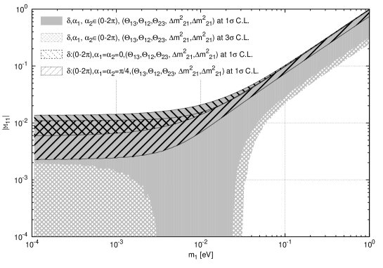
Figure 1: Allowed regions of $|\mathcal{M}^{\nu}_{11}|$ as a function of the lightest neutrino mass in the case of the normal neutrino mass hierarchy.

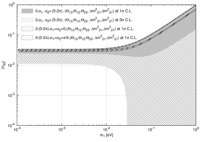
Figure 2: Allowed regions of $|\mathcal{M}^{\nu}_{33}|$ as a function of the lightest neutrino mass in the case of the normal neutrino mass hierarchy.

References

- (1) P. F. Harrison, D. H. Perkins and W. G. Scott, Phys. Lett. B 530, 167 (2002)
- (2) E. Ma, Phys. Rev. D 70, 031901 (2004)
- (3) G. Altarelli and F. Feruglio, Nucl. Phys. B 720, 64 (2005)
- (4) G. Altarelli and F. Feruglio, Nucl. Phys. B 741, 215 (2006)
- (5) K. S. Babu and X. G. He,
- (6) I. de Medeiros Varzielas, S. F. King and G. G. Ross, Phys. Lett. B 644, 153 (2007)
- (7) W. Grimus and L. Lavoura, JHEP 0904, 013 (2009)
- (8) R. N. Mohapatra, S. Nasri and H. B. Yu, Phys. Lett. B 639, 318 (2006)
- (9) C. S. Lam, Phys. Rev. Lett. 101, 121602 (2008)
- (10) F. Bazzocchi and S. Morisi, Phys. Rev. D 80, 096005 (2009)
- (11) F. Feruglio, C. Hagedorn, Y. Lin and L. Merlo, Nucl. Phys. B 775, 120 (2007) [Nucl. Phys. 836, 127 (2010)]
- (12) P. D. Carr and P. H. Frampton, hep-ph/0701034.
- (13) K. Abe et al. [T2K Collaboration], Phys. Rev. Lett. 112, 061802 (2014)
- (14) F. P. An et al. [Daya Bay Collaboration], Phys. Rev. Lett. 112, 061801 (2014)
- (15) P. Adamson et al. [MINOS Collaboration], Phys. Rev. Lett. 110, no. 25, 251801 (2013)
- (16) J. K. Ahn et al. [RENO Collaboration], Phys. Rev. Lett. 108, 191802 (2012)
- (17) B. Dziewit, S. Zajac and M. Zralek, Acta Phys. Polon. B 44, no. 11, 2353 (2013).
- (18) H. Nishiura, K. Matsuda and T. Fukuyama, Phys. Rev. D 60, 013006 (1999)
- (19) Z. z. Xing, Phys. Lett. B 530, 159 (2002)
- (20) Z. z. Xing, Phys. Lett. B 539, 85 (2002)
- (21) W. Grimus, PoS HEP 2005, 186 (2006)
- (22) W. Grimus, A. S. Joshipura, L. Lavoura and M. Tanimoto, Eur. Phys. J. C 36, 227 (2004)
- (23) L. Lavoura, Phys. Lett. B 609, 317 (2005)
- (24) W. Grimus and P. O. Ludl, J. Phys. G 40, 055003 (2013)
- (25) B. Dziewit, S. Zajac and M. Zralek, Acta Phys. Polon. B 42, 2509 (2011)
- (26) D. V. Forero, M. Tortola and J. W. F. Valle, Phys. Rev. D 86, 073012 (2012)
- (27) G. L. Fogli, E. Lisi, A. Marrone, D. Montanino, A. Palazzo and A. M. Rotunno, Phys. Rev. D 86, 013012 (2012)
- (28) M. C. Gonzalez-Garcia, M. Maltoni, J. Salvado and T. Schwetz, JHEP 1212, 123 (2012)
- (29) A. Merle and W. Rodejohann, Phys. Rev. D 73, 073012 (2006)
- (30) W. Grimus and P. O. Ludl, JHEP 1212, 117 (2012)
- (31) M. Gozdz, W. A. Kaminski and F. Simkovic, Acta Phys. Polon. B 37 (2006) 2203