A posteriori error estimation for the -curl problemAndy T. S. Wan, and Marc Laforest \newsiamremarkhypothesisHypothesis
A posteriori error estimation for the -curl problem††thanks: This work was supported by FQNRT, NSERC and MITACS.
Abstract
We derive a posteriori error estimates for a semi-discrete finite element approximation of a nonlinear eddy current problem arising from applied superconductivity, known as the -curl problem. In particular, we show the reliability for non-conforming Nédélec elements based on a residual type argument and a Helmholtz-Weyl decomposition of . As a consequence, we are also able to derive an a posteriori error estimate for a quantity of interest called the AC loss. The nonlinearity for this form of Maxwell’s equation is an analogue of the one found in the -Laplacian. It is handled without linearizing around the approximate solution. The non-conformity is dealt by adapting error decomposition techniques of Carstensen, Hu and Orlando. Geometric non-conformities also appear because the continuous problem is defined over a bounded domain while the discrete problem is formulated over a weaker polyhedral domain. The semi-discrete formulation studied in this paper is often encountered in commercial codes and is shown to be well-posed. The paper concludes with numerical results confirming the reliability of the a posteriori error estimate.
keywords:
finite element, a posteriori, error estimation, Maxwell’s equations, nonconforming, nonlinear, Nédélec element, p-curl problem, eddy current, divergence free35K65, 65M60, 65M15, 78M10
1 Introduction
The optimal design of the next generation of high-temperat-
ure superconductor (HTS) devices will require fast and accurate approximations of the time-dependent magnetic field
inside complex domains [22]. Potential devices include, among others, passive current-fault limiters, MagLev trains and power links in the CERN accelerator.
In a superconductor, any reversal of variation rate in the magnetic field generates a strong front in the current density profile, as well as a discontinuity
in the magnetic field profile, which is not traditionally encountered in computational electromagnetism. It is therefore clear that a posteriori error estimators
can play an important role in the simulation of such devices; first to achieve design tolerances and secondly to implement adaptive mesh refinement.
At power frequencies of the applications concerned, and when the operating conditions are such that we do not exceed significantly the critical current of superconducting wires, the eddy current problem with the so-called power-law model for the resistivity adequately describes the evolution of the magnetic field for by
| (1) | ||||
| (2) |
where is known and the resistivity is modeled by
| (3) |
for some positive material properties and typically between and . The model also includes initial conditions and boundary conditions. Although the boundary conditions are often imposed indirectly by means of a global current constraint, this work will focus on straightforward, but more restrictive, tangential boundary conditions
where is the exterior normal along the boundary. For consistency, the initial conditions and the source term must be divergence free. More general boundary conditions were studied by Miranda et al. [30]. The precise assumptions leading to this model can be found in [27] and a description of how this macroscopic model relates to microscopic models of superconductivity can be found in [11].
There is an obvious analogy between the operator of the model (1) and the -Laplacian, namely . Researchers, Yin [45, 46], as well as Miranda, Rodrigues and Santos [30] have exploited this analogy in order to construct a well-posedness theory for the continuous problem. The key parts of that theory is the observation that the -curl is monotone and the domain must have a smooth boundary. Formal convergence as of the power-law model to the Bean model has also been established in 2D [6] and in 3D [47]. Smoothness of the boundary is an essential constraint coming from the harmonic analysis in spaces [25, 31, 36].
As far as we know, the theory of convergence of finite element approximation using Nédélec elements, within the same framework of Yin, has yet to be established. On the other hand, using an electric field formulation of the -curl problem, Slodic̆ka and Janíková showed convergence results within spaces for backward Euler semi-discretizations and fully-discretizations using linear Nédélec elements in [39, 23, 24]. However, their work has only focused on a priori error estimates.
The main result of this paper, an a posteriori error estimate, appears to be the first residual-based error estimate for the problem (1). In the work of Sirois et al. [38], an explicit adaptive time-stepping scheme was handled by SUNDIALS [26] which contains sophisticated but generic error control strategies. The error estimates presented in this paper are residual based and resemble the a posteriori error estimators one finds for linear or linearized problems [42]. In fact, our results differ from those of Verfürth in our treatment of the non-conformity of the approximation and in our circumvention of linearization. Error estimation for FE approximate solutions of the -Laplacian is quite well-developed and in fact, we mention the important work on reliable and efficient error estimation using quasi-norms [28, 9, 10, 15, 7]. In recent work of El Alaoui et al. [2], quasi-norm error estimates were obtained by re-interpreting the estimators in terms of flux corrections satisfying specific properties. It appears that their approach could be adapted to the -curl using the tools we presented here to handle non-conformity issues. The error estimate presented here also controls the error in an important quantity of interest, the AC loss over one cycle. We have included a proof of the well-posedness for the straightforward semi-discretization often considered within the engineering community. Numerical results are presented to assess the quality of the error estimators. These experiments confirm the reliability of the error estimators on a class of moving front solutions in D.
The novelty of this paper is the treatment of the lack of conformity of the Nédélec element approximations. Inspired largely by the work of Carstensen, Ju and Orlando on the issue [8], we have found that coercive estimates are sufficient to obtain reliable error estimates. This is in stark contrast to most nonlinear problems which require a linearization of the operator in a neighborhood of the numerical solution. Given that the semi-discretization considered here is also found in commercial codes, and that the a posteriori error estimators of this paper are straightforward to implement, it appears that this work could be of interest to the engineering community.
The a posteriori error estimate also includes an interesting non-conformity error originating from the geometric defect between the approximation of the domain , required for the continuous problem, by the polyhedral domain required for the finite element formulation. Even with the use of curved elements approximating the boundary, such a geometric defect could not be eliminated. This difficulty, which appears to be specific to nonlinear harmonic analysis in spaces [25], is carefully analyzed and reduced to a boundary term on mesuring our inability to represent the discrete solution over a domain. Morevover, the techniques used required that the polyhedral mesh be strictly included inside the domain of the continuous problem. The paper includes a novel construction of a family of uniformly regular polyhedral domains strictly inside a domain, based on the work of Delfour [13], Oudot, Rineau and Yvinec [34], and Talmor [40].
The paper is organized as follows. The second section presents a brief review of the functional analysis required for the a posteriori error estimation. In Section 3, for the sake of completeness we include a demonstration of the well-posedness of our semi-disretization of the -curl problem. The fourth section contains the proof of the main theorem. It is later extended in Section 5 to the control of the AC loss. The last section describes numerical results obtained when comparing the error estimator to the exact error for a class of moving front solutions using the method of manufactured solutions and as well as convergence results for a backward Euler discretization. In Appendix A, we have extended the a posteriori error estimator to the case of non-homogeneous tangential boundary conditions, exploiting again properties unique to the -Laplacian and the -curl problem.
2 Preliminaries
This section reviews the main functional spaces over which the -curl problem is examined and it states the strong and weak forms of the problem. The triangulation of the domain is carefully discussed since it involves a non-conformity issue important to the -curl problem. A brief review of the finite element discretization of the -curl is given. This section concludes with a detailed presentation of the two main technical tools, namely the Helmholtz-Weyl decomposition over spaces and the quasi-interpolation operator of Schöberl [35].
Let and be a bounded Lipschitz domain in . Let be a nonnegative integer and for denote its integer part as . Throughout, we denote as the Hölder conjugate exponent of satisfying . Recall the following well-known Sobolev spaces [1].
For the -curl problem, we will see later that minimal regularity suggests that we consider the following spaces with being a bounded domain; see [31, 4] for more details on their properties and equivalent norms.
Above, is the continuous boundary trace operator and , are the continuous tangential and normal trace operators satisfying [16, Corollary B.57 and B.58]:
| (4) | ||||
| (5) | ||||
For sufficiently smooth functions and , these trace operators are simply , and . Later, we will need the stability bound below [1].
Lemma 2.1.
Let be a bounded domain with a Lipschitz boundary. If , then the boundary trace operator is a continuous linear operator, i.e. there exist a constant such that,
| (6) |
As is customary for spaces, we write as and similarly we write and as and , respectively.
If , we denote the pairing
and define the nonlinear operator ,
| (7) |
Indeed, by Holder’s inequality, these pairings are well-defined since,
Over the time interval , the -curl problem arising from applied superconductivity is the following nonlinear evolutionary equation:
| (8) |
where , is the nonlinear resistivity modeled by an isotropic power law and is a material dependent constant. Moreover, it is assumed that and for all in a manner to be made precise later.
The weak formulation of the -curl problem is:
Given a bounded domain, and , find satisfying and
| (9) |
The well-posedness of the weak problem was established in the work of Yin et al. [46, 47]. The stability of the solution is characterized by two inequalities from Lemma 3.2 of [47], one of which is given by
| (10) | ||||
We demonstrate a similar bound for our approximate solution in Theorem 3.1.
2.1 Approximating a domain
Being restricted to a domain , in part due to the well-posedness of the -curl problem, we observe that the domain of the polyhedral mesh cannot be equal to , and therefore that the solution to (9) and any finite element approximation cannot be defined over the same domain. When comparing and , this introduces a geometric non-conformity that requires us to construct a polyhedral mesh that approximates the domain sufficiently well. The construction of the mesh will exploit the fact that domains are (nearly) those with the weakest regularity for which tubular neighborhoods can be defined. For the sake of simplicity, the description will be given only in although the modifications to should be obvious.
Let be a collection of shape-regular triangularization of where with being the largest diameter over all . Denote as the polyhedral mesh with the obvious constraints that are required to ensure that the set of faces and edges of are well-defined. Also for each , denote as the diameter of and as the diameter of the largest inscribed sphere within . By definition of shape-regularity of , for all . Moreover, for each face on , we also denote as the diameter of and to be the diameter of the largest inscribed circle within . The following lemma is obtained by combining the trace theorem of Lemma 2.1 with a standard scaling argument.
Lemma 2.2.
Let and be any face on . If , then there exists a constant independent of and such that,
| (11) |
Due to the geometric non-conformity, we will further be interested in a special class of triangulation of . For a bounded domain , we define an interior mesh to be a triangulation of the domain for which the union of all tetrahedron is strictly contained in . If is a convex domain and the vertices of lies within , then clearly is an interior mesh of . For a fixed nonconvex bounded domain , the existence of a sequence of triangulations for which the volume of the defect vanishes uniformly, in some sense, is far from obvious. We begin with a fundamental result of Delfour [13], citing Lemma 2.1 from [14].
Theorem 2.3.
Let be a bounded domain with a non-empty boundary . There exists a number , an open neighborhood of , and a bi-Lipschitzian map
satisfying
-
i)
the map is the identity over ;
-
ii)
for each the image of the map is a hypersurface;
-
iii)
for each fixed , the derivative is the exterior normal to the boundary at ;
-
iv)
for all , the image is inside .
For domains with weak regularity, there exists a triangulation algorithm developed by Oudot, Rineau and Yvinec [34] which constructs a mesh arbitrarily close to the boundary. The algorithm only requires an oracle that (i) determines if a point is inside the domain, and (ii) computes the intersection point between the boundary and a segment in generic position. This algorithm has been implemented in CGAL [41] and distinguishes itself from conventional algorithms that are usually restricted to polyhedral domains. We present here a form of their result specifically adapted to our situation.
Theorem 2.4.
Let be a bounded domain with a non-empty boundary . There exists a positive constant and a Lipschitz sizing field on ,
such that for every , there exists a triangulation of an interior mesh of satisfying
-
i)
;
-
ii)
for all faces along the boundary of the mesh,
(12) -
iii)
the triangulation is shape-regular, that is
Proof 2.5.
For every positive value of less than , define the domain
We will now construct a triangulation of that guarantees that the union of the tetrahedrons of the mesh satisfy
| (13) |
The algorithm of Oudot, Rineau and Yvinec allows us to construct a triangulation of a domain, but not necessarily produce an interior mesh. The iterative algorithm begins by choosing a value for the bound on the radius-edge ratio, that is the ratio
| (14) |
where is the length of the shortest edge of . Points are then randomly selected inside and on the boundary . Tetrahedrons and faces on the boundary are selectively refined by inserting the circumcenter and connecting the vertices to the circumcenter until both (12) and (14) are satisfied.
We will show that if a face on the boundary of the mesh satisfies a constraint , then
| (15) |
Choose a face belonging to the boundary of , suppose one of its three vertices is . For a point , define and the smooth function describing, for arc length , the straight line segment connecting to . If is the projection onto the second variable, then the Lipschitz continuity of the inverse of implies that there exists a constant such that
Therefore, if all the vertices belong to and if the face satisfies
| (16) |
for some fixed , then the condition (15) holds and the mesh is strictly inside . Moreover, the constant depends only on the Lipschitz constant of the boundary , and not on . We remark that these observations allow us to assign to each vertex the value , which depends only on , and then construct the sizing field as a piecewise linear interpolant of these values. The inverse of then allows the sizing field over to be defined over .
Finally, we address the shape-regularity of the mesh. In fact, the algorithm by Oudot et al. only produces meshes with bounded radius-edge ratios (14) and these meshes may contain so-called slivers, that is tetrahedrons possessing one vertex close to the plane of the three others vertices yet with angles bounded from below. There exists very efficient algorithms to remove such slivers, but in fact the Sliver Theorem of Talmor states that if a mesh satisfies the radius-edge ratio condition, then there exists a topologically equivalent mesh that is shape-regular [40]. From a mathematical perspective, the shape-regular condition therefore follows from the choice of the constraint .
The main motivation for introducing an interior mesh is the following simple extension result.
Lemma 2.6.
Let be an interior mesh of . For each , its trivial extension by zero defined by
belongs to .
Proof 2.7.
Clearly, . Since and , the tangential jump . So, it follows from (4) that, and clearly .
2.2 Semi-discretization of -curl problem by Nédélec finite elements
In , the -th order Nédélec finite element space of the first kind [33] and with zero tangential trace can be defined as,
| (17) | ||||
| (18) |
where is the space of vector fields with polynomial components of at most degree . Recall that the finite element space is uniquely determined by identifying the degrees of freedom of the surface integral along faces and edges between any two neighboring elements. Since an element-wise defined function that is continuous tangentially along faces and edges is a global function, . Moreover is known to be locally divergence-free, i.e. for , and thus it is an element-wise defined function. Unfortunately, higher order elements will not be in . In any case, can be discontinuous in the normal direction to faces and edges and hence in general is not a global function. In particular, .
This leads us to the non-conforming semi-discrete weak formulation of the -curl problem:
Given and , find
satisfying and
| (19) |
Due to the non-conformity, well-posedness of the semi-discretization does not necessarily follow from the well-posedness of the weak formulation. By a local existence argument and a priori estimate, we show that the semi-discretization is well-posed in Section 3. Note that, while the weak formulation only requires to be in , we need to be continuous in in order apply Picard’s local existence theorem.
2.3 Helmholtz-Weyl decomposition of functions
We now proceed with a rather detailed review of the Helmholtz-Weyl decomposition for spaces. This is needed to address the non-conformity in a manner similar to the work of [8]. The most technical aspects concerning the -curl problem turn out to be related to this decomposition, not only because of the Banach nature of the spaces concerned, but also because it imposes strict limits on the regularity of the boundary.
Define closure of with respect to . A standard formulation of the decomposition is the following.
There exists a positive constant such that for any , there exists and
for which and
| (20) |
When the vector field has zero boundary trace, then the Helmholtz-Weyl decomposition is as follows.
There exists a positive constant such that for any , there exists and for which
and
| (21) |
While the decomposition when can be studied using tools no more complicated than the Lax-Milgram theorem, the case for general is much more subtle.
It has been observed (for example [20, Lemma III 1.2]) that the existence of the Helmholtz-Weyl decomposition of (20)
is equivalent to the solvability of the following Neumann problem over .
Given , find such that for all ,
Similarly, the existence of Helmholtz-Weyl decomposition of (21) is equivalent to the solvability of the Dirichlet problem below.
Given , find such that for all ,
In particular, if is a bounded Lipschitz domain then for some depending on the Lipschitz constant of , it was shown in [17] that the above Neumann problem has a solution in a sharp region near . Similarly, [25] showed that the above Dirichlet problem has a solution in a sharp region near . This implies the Helmholtz-Weyl decomposition does not hold in general for bounded Lipschitz domains, which is unfortunate since such domains do arise in engineering applications of superconductors. Thus, we are forced to restrict to bounded domains, which are consistent with the regularity of the boundary required for the well-posedness of the -curl problem given by [47].
The Helmholtz-Weyl decomposition for was first demonstrated by [44] and for by [19] for smooth bounded domains. For , to the best of our knowledge, the weakest regularity requirement for the Helmholtz-Weyl decomposition to hold are bounded domains [36, 37] and more recently for bounded convex Lipschitz domains [21].
Theorem 2.8.
Theorem 2.9.
We also mention that Amrouche et al. [4] have published an version of the Hodge decomposition for domains with boundary. We now use Theorem 2.8 to derive a new Helmholtz-Weyl decomposition for for bounded domain.
Lemma 2.10.
Let be a bounded simply connected domain and let . Then the following direct sum holds,
In other words, for any , there exists unique and such that satisfying,
| (22) |
Proof 2.11.
Let . Then by Theorem 2.8, for some and . Since , is well defined. Let converging to in . Since and so , then by continuity of the tangential trace operator and so . I.e. .
To show the sum is direct, suppose . Then for some . Since , for all ,
| (23) |
As , . Setting in (23) implies and hence a.e. by Friedrichs’ inequality. I.e. .
Finally, we conclude with the quasi-interpolation operator of Schöberl [35, Theorem 1], which for Nédélec elements plays the same role the Clément operator does for Lagrange elements.
Theorem 2.12.
Consider a bounded polyhedral domain possessing a triangulation . There exists a quasi-interpolation operator with the property: for any , there exists and such that,
| (24) |
Moreover, on each there exists an element patch of and a constant depending only on the shape constants of the elements in such that satisfy
| (25) | ||||
| (26) |
3 Well-posedness of the semi-discretization
This section contains a short proof of the well-posedness of the semi-discrete weak formulation of (19). The well-posedness is not required for the construction of the a posteriori error estimators in the following section, and so this section can be read independently of the others. Nevertheless, for the sake of accessibility, this topic is best discussed first.
Theorem 3.1.
There exists a unique solution satisfying the semi-discrete weak formulation of (19). Moreover, the stability estimates hold,
| (27) | ||||
| (28) | ||||
Proof 3.2.
The space of -th order Nédélec elements is a closed subspace of and we restrict the norm of to it,
By Riesz representation theorem for functions, there is an isometry , also known as the Riesz map. Then we can view the semi-discrete weak formulation of (19) as seeking an unique solution to the first order ODEs,
| (29) |
The proof proceeds in 2 steps. First, we show local existence for (29). Second, we extend its interval of existence to by a priori estimates.
To show local existence, we verify that the right hand side of (29) is continuous in and locally Lipschitz continuous in . Indeed, since with and , for all . This implies for any and ,
It follows that,
which tends to as . This shows is continuous in .
Now recall from [5, Lemma 2.2], that the following equality holds for some ,
So for any , it follows from the above inequality and Hölder’s inequality with so that , and ,
Moreover, the case for follows directly from Cauchy-Schwarz inequality. Thus, we have that for any compact subset and any ,
This shows that is locally Lipschitz continuous in . Thus, by Picard’s existence theorem, there exists an unique local solution to (19), with .
Finally, we extend to by showing the following a priori estimates. At every , we have . Setting now in (19), and combining with Young’s inequality and Gronwall’s inequality implies
Thus, taking supremum on the left hand side and setting shows the stability estimate (27), which implies can be extended to . Similarly, the second stability estimate (28) follows by setting in (19) and noting that .
4 A posteriori error estimator
This section contains the main result of this paper, Theorem 4.5. The proof follows the usual residual-based approach except for the treatment of the non-conformity and nonlinearity. We begin with Lemma 4.1 which enables us to test the weak formulation with a larger test space. This is then used to bound the error, as stated in Theorem 4.3. Afterwards, stability estimates for both the trace operator and Schöberl’s quasi-interpolation operator allow us to combine the local estimate into a global estimate of Theorem 4.5.
Lemma 4.1.
Consider a simply connected bounded domain and a source term . Assume that is a weak solution to (9), then
| (30) |
Proof 4.2.
Due to the discrepancy of the tangential boundary condition between and on , we will also need to decompose into two contributions which are associated with the interior and boundary elements of . Specifically for , can be expressed as linear combinations of global shape functions by assigning the same degrees of freedom along tangential components of on common edges and faces [32, 16],
where are some fixed polynomial basis, and the face and volume degrees of freedom are present only when and , respectively. Denoting and as the set of faces and edges on the boundary and and as the set of faces and edges on the interior part of , we can write , where and are interior and boundary parts of defined as
We note that by unisolvency of the degrees of freedom for Nédélec elements, , and so . Moreover, where .
We are now in a position to prove a key theorem of a posterior error estimation for the -curl problem.
Theorem 4.3.
Consider a simply connected bounded domain and a source term . Let be shape-regular triangulations satisfying the interior mesh property provided by Theorem 2.4. If and are respective solutions to (9) and (19), then there exists depending only on shape regularity condition of Theorem 2.4 such that for any ,
| (31) | |||
where is the boundary part of , the Schöberl quasi-interpolant of ,
| (32) | ||||
Here, and denote the tangential and normal jump of and across a common face with exterior normals .
Proof 4.4.
Since and , we can extend by zero using Lemma 2.6 so that . It follows then for any and ,
| (33) |
Since , the restriction and so we can set to be the quasi-interpolant of Theorem 2.12. Moreover, there exists and for which and the estimates (25) and (26) hold. It remains to estimate . For this, we apply Green’s formula (4) and (5) to obtain
| (34) |
where the residuals are defined by
Indeed, is the standard interior local residual term while and measure respectively the normal and tangential discontinuity of and across neighbouring elements. Moreover, and measures the boundary defects of and along the boundary faces of . We observe that at each , implies that the first term in satisfies but the second term vanishes only for first order Nédélec elements. Hence, the residual measures the defect in the divergence constraint at the discrete level, namely by
Next, we proceed to estimate each term in the sum of (34) by using Holder’s inequality, (25), and (26). We use the convention that the constant may change from one line to the next and only depends on the shape-regularity of .
| (35) |
To bound the terms, we proceed in the same way
| (36) |
For the terms, we begin with a stability estimate. Using (11) and for shape-regular , we find
Employing this last estimate, we obtain
| (37) |
We can bound the boundary terms in the same manner and obtain
| (38) |
Similarly to the previous stability estimate, using (11) and the shape-regularity of , one can show that
Applying this to the term, one finds
| (39) |
Similarly, we can bound the boundary terms and obtain
| (40) |
Thus, combining (33)-(40), we have shown the desired result.
Now we show the a posteriori error estimators in Theorem 4.3 are reliable in the following sense.
Theorem 4.5.
Let , and be as stated in Theorem 4.3 and denote the error as and . Then there exists some positive constants and such that,
where and are non-conforming geometric errors defined as,
with .
Above, and are called non-conforming geometric errors since and . Specifically, measures with the geometric defect of between the embedded polyhedral domain and the domain, while arises from the boundary data defect of along .
Proof 4.6.
Since , setting in (31) gives,
| (41) | |||
We proceed to estimate each term on both sides of (41). First, we can bound from below the second term on the left hand side of (41) by the following inequality [12, eqn 24], where for some ,
Thus, setting and integrating the above inequality above gives the coercivity estimate
| (42) |
Second, to bound from above the residual term on the right hand side of (41), note that is a projection on a finite dimensional space and thus is bounded on with the operator norm . Moreover, by (25) and (26), there are constants such that for each ,
| (43) | ||||
| (44) | ||||
And since each overlaps with finitely many , is bounded as (43) and (44) implies for some positive constant ,
| (45) | ||||
| (46) |
Using (45), the first residual term in (32) can be bounded above with the help of Young’s inequality for any and some positive constant ,
where and the last inequality follows from and with . Similarly, using (46), for an arbitrary positive , the second residual term in (32) can be bounded above as
where and the last step follows from with . Combining these two estimates for the residual of (32), we have for that for some positive constant depending on and some positive constant depending on but not ,
Finally, combining with (42), (41) becomes,
| (47) | ||||
Thus, for sufficiently small , inequality (47) implies that there exists positive constants and for which
So multiplying by and integrating yields
| (48) |
since for with . Taking the supremum over all of equation (48) gives the desired result.
5 A posteriori error estimate for AC loss
For many engineering applications, the quantity of interest is the AC loss over one period ,
In particular, we wish to derive a posteriori error estimates for . To do this, we first derive the following elementary estimate and subsequently use it to show the error for is related to the a posteriori error estimates derived previously.
Lemma 5.1.
Assume and , then for any functions , , we have
Proof 5.2.
For any , applying the mean value theorem for the function on implies there exists satisfying
Thus, integrating over gives,
Theorem 5.3.
6 Numerical results
We present numerical results in 2D supporting the reliability of the error estimators presented in Section 4. In the following, the -curl problem is discretized in space using first order Nédélec elements and in time using the backward Euler method. While higher order time stepping schemes can be used, the discretization error is shown to be dominated by the spatial errors due to the low order approximation of first order Nédélec elements. The fully discrete formulation was implemented in Python using the FEniCS package [3]. For simplicity, we have scaled the units such that the material parameter is set to unity.
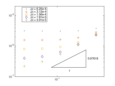
6.1 Numerical verification of first order convergence
We verify numerically first order convergence on the unit circle for a smooth radially symmetric solution with the forcing term Specifically, the constants are parameters to be chosen, is the radial cylindrical coordinate and is the azimuthal unit vector. Note that by radial symmetry, is necessarily divergence-free. For these tests, we have fixed and the final time =5e-3.
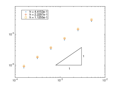
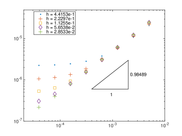
For , the solution is linear in both space and time. Since both first order Nédélec elements and backward Euler method are exact for linear functions, it was observed that the FE solution was accurate up to machine precision.
6.2 Numerical verification of reliability of a posteriori error estimators
Next, we numerically verify the reliability of the error estimators presented in Section 4. We will first look at the case of a convex domain given by the unit circle and then consider a nonconvex domain given by an annulus. Finally, we look at a moving front case with sharp gradient often encounter in practice for the -curl problem. In all cases, the computational mesh was constructed to be an interior mesh of using the native mesh generator of FEniCS.
6.2.1 Convex domain - circle
For the unit circle , we generate an interior mesh by specifying the number of perimeter segments of the polygonal domain to be inscribed inside the unit circle. For instance, if the number of segments is with equal length and the perimeter vertices lies on the unit circle, then elementary trigonometry shows that , which converges to as . In the following, as we refine the mesh by reducing by half, we correspondingly also double the number of segments on the perimeter of .
On and , we employed a radially symmetric inward moving front solution of the form with,
where is a parameter to be chosen. It can be checked that the current density has the form with
Thus, the corresponding forcing term is given by,
The motivation for choosing this family of manufactured solutions originates from an exact analytical solution of Mayergoyz [29] of the -curl problem in 1D. In particular, it is known that the parameter for the 1D case and so for large values of . Moreover, it can be seen that as approaches , the current density has steeper gradients and converges pointwise to a discontinuous function. In fact for , it can be checked that if and only if .111Since where is the distance away from the front, . Thus, for close to , we do not expect the FE approximation using Nédélec elements to be accurate, since its interpolation error requires to be at least a function [16, Theorem 1.117]. For these reasons, we have focused on a case satisfying . More specifically, we have fixed , , =5e-4.
The integration in time was computed numerically using the composite midpoint rule. Also note that, since the initial field , the initial error is identically zero. Moreover, recalling that first order Nédélec elements are element-wise divergence free, we omitted computing as it is identically zero. Finally, the boundary elements were refined to be sufficiently small such that the term was negligible in the computation of .
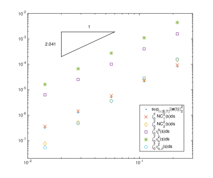
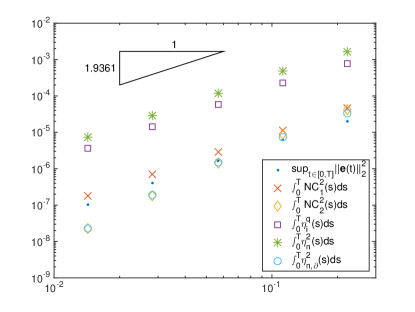
In Figure 3, the error in , nonconforming geometric error estimators and estimators , and from Theorem 4.5 are plotted for various mesh sizes . Note that we have omitted showing , , and as their values were observed to be near machine precision zero due to their small magnitude and/or their dependence on the exponent of . As illustrated, we observed quadratic order of convergence in for both the error and estimators showing agreement of the reliability of the estimators. This is consistent with the first order convergence of Section 6.1, since the error quantity under consideration is squared with respect to the norm. We also observed that the error estimators and decreases at a faster rate due to the refinement of .
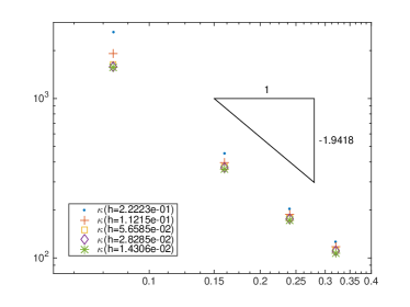
In the absence of knowledge on the constants and from Theorem 4.5, we can still measure the reliability of the error estimators by the quantity 222For stationary problems, is usually called the effectivity index of the error estimators. defined as the ratio of estimators over the errors by,
Ideally, for efficient mesh adaptivity, one would like to have . However, due to the unknown constants inherent in the present residual type error estimation and the dependence on due to time integration, we can only expect to decrease with . In particular, since the error estimators from Theorem 4.5 are reliable, then should be bounded below by the constant , where increases in the worst case exponentially with respect to .
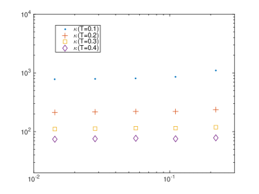
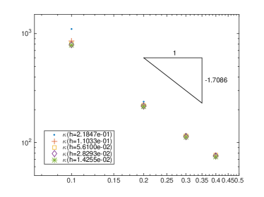
In Figure 4a, is shown to be largely independent of and decreases with . This suggests that the error estimators are comparable to the actual error up to a factor of . Moreover, from Figure 4b, we see that which suggests that the exponential dependence on for the constant in Theorem 4.5 may be sharpened to in this case.
6.2.2 Nonconvex domain - annulus
Next we consider a nonconvex domain given by the annulus region . We construct an interior mesh by specifying the number of perimeter segments on the outer radius of and removed a polygonal region with the number of perimeter segments inscribed on the inner radius . In order the guarantee , was chosen to be slightly larger than so that the removed polygonal region covers the removed part of the annulus region of . For instance, if the perimeter segments on the inner radius is of equal length, then elementary trigonometry shows that the inner radius is which converges to as . Similar to the unit circle case, as we refine the mesh by reducing by half, we correspondingly also double the number of segments on both the number of inner and outer perimeter segments and of .
On the annulus domain, we used a similar manufactured solution as the unit circle except the radially symmetric moving front solution is moving outward from . The choice was made to differentiate the inward-moving solution of the unit circle case. Specifically, it has the form with,
where we have again chosen , and .
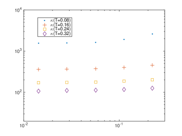
In Figure 5, we observed similar quadratic order of convergence in for both the error and estimators. We also observed ’s independence of in Figure 6a and rate of decrease in in Figure 6b, where in this case.
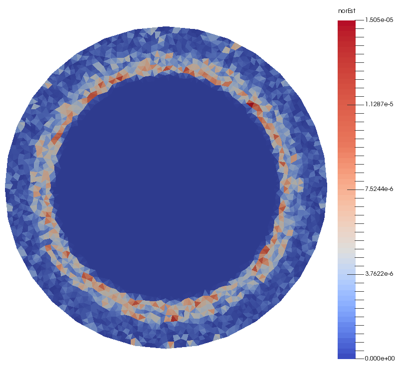
6.2.3 Nonsmooth case
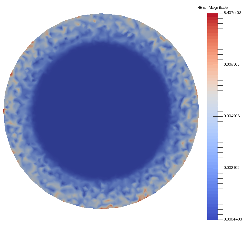
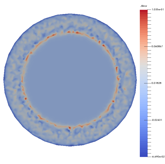
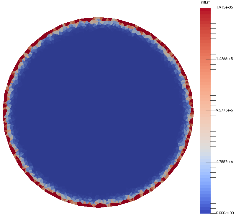
Finally, we look at a case for which . For this, we consider again the manufactured solution on the unit circle domain and we chose and so that . The purpose here is to compare qualitatively between the error and estimators even in this nonsmooth case. As illustrated in Figure 8 and Figure 10, the region where the local estimators are largest agrees with regions where the sharp gradient occurs in the current density . Moreover, in Figure 7 and Figure 9, the local estimators identified the boundary region as where the increasing magnetic field was being applied.
7 Conclusion
This paper has presented an original a posteriori residual-based error estimator for a nonlinear wave-like propagation problem modeling strong variations in the magnetic field density inside high-temperature superconductors. The techniques used circumvent the non-conformity of the numerical approximations in a simple manner and the nonlinearities are handled using only coercive properties of the spatial operator, and without any linearization. Preliminary numerical results in two space dimensions indicate that the residuals are asymptotically exact, up to a constant.
An important avenue for future research would be to develop error estimators which are both reliable and efficient. The work of Carstensen, Liu, and Yan on quasi-norms for the -Laplacian appears to be the next natural step, given the similarities in the analytic framework underlying both problems [28, 9, 10]. We also mention the recent optimality results of Diening and Kreuzer on adaptive finite element methods for the -Laplacian [15, 7] and of Alaoui, Ern and Vohralîk on a posteriori error estimates for monotone nonlinear problems [2]. Moreover, further investigation is needed concerning the efficiency for solving the nonlinear discrete problems arising from successive adaptive mesh based on such error estimators. At the moment, the optimal design of new high temperature superconducting devices is limited by the high computational cost of such simulations, and all means of improving this efficiency should be examined in hopes of removing this bottleneck.
Appendix A Non-homogeneous tangential boundary condition
We can account for the non-homogeneous tangential boundary conditions on by establishing a “Duhamel’s principle” for the -curl problem. The novelty here is in the treatment of the homogeneous auxiliary variables and in the nonlinearity.
Denote as the space of curl-free functions. It suffices to show the following:
Theorem A.1.
Let be a bounded simply-connected domain in and let with . For any with , there exists a function with and a function such that .
Indeed, if such decomposition exists, since is curl- and divergence-free, the non-homogeneous -curl problem reduces to the homogeneous -curl problem,
| (51) |
Proof A.2.
Given a function , we construct in three main steps.
First, let be such that . Such exists by the surjectivity of the image space .
Second, let be the solution to the problem:
| (52) |
Such a function exists if the following two conditions hold [16]:
| (53) |
and if for all ,
| (54) |
We first show the inf-sup condition. From the Helmholtz decomposition of Theorem 2.8, for , there exists and such that with for some constant . In particular, for any , . This implies that for any ,
Since the norm is equivalent to for , dividing the above inequality by and taking the infimum over shows the inf-sup condition (53) is satisfied.
We now explain why condition (54) also holds. For , by Poincaré’s inequality the condition implies that almost everywhere. Thus, a unique solution to (52) exists.
Third, let be the solution to the problem:
| (55) |
Similarly, such a function exists if the following two conditions hold:
| (56) |
and if for all ,
| (57) |
By Lemma 5.1 of [4], the inf-sup condition (56) is satisfied. Moreover, since for , implies a.e. by the equivalence of the semi-norm on ; see Corollary 3.2 of [4]. Hence, a unique solution to (55) exists.
Combining these three functions, we define
Note that , since and . Since is divergence-free, as satisfies (52). Moreover, since satisfies (55); i.e. . Thus, with .
Finally, defining and noting , . This shows that as claimed.
Acknowledgments
The authors would like to thank Frédéric Sirois for the countless discussions on the physical model of the -curl problem. Also, the first author would like to thank Gantumur Tsogtgerel for his valuable comments. Portions of results of Section 4 and Section 5 were included in the first author’s PhD thesis [43]. The authors would also like to thank the anonymous reviewers for their time and helpful suggestions to improve the paper.
References
- [1] R. A. Adams and J. F. F. Fournier, Sobolev Spaces, vol. 140 of Pure and Applied Mathematics, Academic Press, Netherlands, 2003.
- [2] L. E. Alaoui, A. Ern, and M. Vohralîk, Guaranteed and robust a posteriori error estimates and balancing discretization and linearization errors for monotone nonlinear problems, Comp. Methods Appl. Mech. Eng., 200 (2011), pp. 2782–2795.
- [3] M. Alnæs, J. Blechta, J. Hake, A. Johansson, B. Kehlet, A. Logg, C. Richardson, J. Ring, M. Rognes, and G. Wells, The fenics project version 1.5, Archive of Numerical Software, 3 (2015), doi:10.11588/ans.2015.100.20553, http://journals.ub.uni-heidelberg.de/index.php/ans/article/view/20553.
- [4] C. Amrouche and N. E. H. Seloula, -theory for vector potentials and Sobolev’s inequalities for vector fields: Application to the Stokes equations with pressure boundary conditions, Mathematical Models and Methods in Applied Sciences, 23 (2013), pp. 37–92.
- [5] J. W. Barrett and W. B. Liu, Finite element approximation of the parabolic p-Laplacian, SIAM J. Numer. Anal., 31 (1994), pp. 413–428.
- [6] J. W. Barrett and L. Prigozhin, Bean’s critical-state model as the limit of an evolutionary -Laplacian equation, Nonlinear Analysis, 42 (2000), pp. 977–993.
- [7] L. Belenki, L. Diening, and C. Kreuzer, Optimality of an adaptive finite element method for the p-laplacian equation, IMA J Numer Anal, 32 (2012), pp. 484–510.
- [8] C. Carstensen, J. Hu, and A. Orlando, Framework for the a posteriori error analysis of nonconforming finite elements, SIAM J. Numer. Anal., 45 (2007), pp. 68–82.
- [9] C. Carstensen and R. Klose, A posteriori finite element control for the p-Laplace problem, SIAM J. Sci. Comput., 25 (2003), pp. 792–814.
- [10] C. Carstensen, W. B. Liu, and N. N. Yan, A posteriori error estimates for finite element approximation of parabolic p-Laplacian, SIAM J. Numer. Anal., 43 (2006), pp. 2294–2319.
- [11] S. J. Chapman, A hierarchy of models for type-II superconductors, SIAM Review, 42 (2000), pp. 555–598.
- [12] S. S. Chow, Finite element error estimates for non-linear elliptic equations of monotone type, Numerische Mathematik, 54 (1989), pp. 373–393.
- [13] M. C. Delfour, Tangential differential calculus and functional analysis on a submanifold, in Differential-geometric methods in the control of partial differential equations, R. Gulliver, W. Littman, and R. Triggiani, eds., vol. 268, Amer. Math. Soc., Providence, R. I., 2000, pp. 83–115. Contemporary Mathematics.
- [14] M. C. Delfour, Representations, Composition, and Decomposition of -hypersurfaces, in Optimal Control of Coupled Systems of Partial Differential Equations, K. Kunisch, G. Leugering, J. Sprekels, and F. Trôltzsch, eds., vol. 158, Birkhäuser Basel, 2009, pp. 85–104. International Series of Numerical Mathematics.
- [15] L. Diening and C. Kreuzer, Linear convergence of an adaptive finite element method for the p-Laplacian equation, SIAM J. Numer. Anal., 46 (2008), pp. 614–638.
- [16] A. Ern and J.-L. Guermond, Theory and practice of finite elements, vol. 159 of Applied Mathematical Sciences, Springer, New York, 2004.
- [17] E. Fabes, O. Mendez, and M. Mitrea, Boundary layers on Sobolev-Besov spaces and Poisson’s equation for the Laplacian in Lipschitz domains, Journal of Functional Analysis, 159 (1998), pp. 323–368.
- [18] G. Folland, Real Analysis : Modern Techniques and Their Applications, Pure and Applied Mathematics, Wiley-Interscience, New York, 1984.
- [19] D. Fujiwara and H. Morimoto, An -theorem for the Helmholtz decomposition of vector fields, J. Fac. Sci. Univ. Tokyo, Sect. Math, 24 (1977), pp. 685–700.
- [20] G. P. Galdi, An Introduction to the Mathematical Theory of the Navier-Stoke Equations, Springer, 2nd ed., 2011.
- [21] J. Geng and Z. Shen, The Neumann problem and Helmholtz decomposition in convex domains, Journal of Functional Analysis, 259 (2010), pp. 2147–2164.
- [22] F. Grilli, E. Pardo, A. Stenvall, D. N. Nguyen, W. Yuan, and F. Gömöry, Computation of Losses in HTS Under the Action of Varying Magnetic Fields and Currents, IEEE Trans. Appl. Supercond., 24 (2014), p. 8200433.
- [23] E. Janíková and M. Slodic̆ka, Convergence of the backwards Euler method for type-II superconductors, J. Math. Anal. Appl., 342 (2008), pp. 1026–1037.
- [24] E. Janíková and M. Slodic̆ka, Fully discrete linear approximation scheme for electric field diffusion in type-II superconductors, J. Comput. Appl. Math., 234 (2010), pp. 2054–2061.
- [25] D. Jerison and C. E. Kenig, The Inhomogeneous Dirichlet problem in Lipschitz Domains, Journal of Functional Analysis, 130 (1995), pp. 161–219.
- [26] L. L. N. Laboratory, SUNDIALS : Suite of Nonlinear and Differential/Algebraic equation Solvers, http://computation.llnl.gov/casc/sundials/main.html, 2002.
- [27] M. Laforest, F. Sirois, and A. Wan, An adaptive space-time finite element discretization for the -curl problem from applied superconductivity, p. 30. In preparation.
- [28] W. B. Liu and N. N. Yan, Quasi-norm local error estimates for p-Laplacian, SIAM J. Numer. Anal., 39 (2001), pp. 100–127.
- [29] G. P. Mikitik, Y. Mawatari, A. T. S. Wan, and F. Sirois, Analytical methods and formulas for modeling high temperature superconductors, Applied Superconductivity, IEEE Transactions on, 23 (2013), p. 8001920.
- [30] F. Miranda, J.-F. Rodrigues, and L. Santos, On a -Curl system arising in electromagnetism, Discr. Cont. Dyn. Syst., 5 (2012), pp. 605–629.
- [31] M. Mitrea, Sharp Hodge decompositions, Maxwell’s equations, and vector Poisson problems on nonsmooth, three-dimensional Riemannian manifolds, Duke Math. J., 125 (2004), pp. 467–547.
- [32] P. Monk, Finite element methods for maxwell’s equations, (2003).
- [33] J.-C. Nédélec, Mixed finite elements in , Numer. Math., 35 (1980), pp. 315–341.
- [34] S. Oudot, L. Rineau, and M. Yvinec, Meshing volumes bounded by smooth surfaces, in Proceedings of the 14th International Meshing Roundtable, B. W. Hanks, ed., Springer Berlin Heidelberg, Berlin, Heidelberg, 2005, pp. 203–219.
- [35] J. Schöberl, A posteriori error estimates for Maxwell equations, Mathematics of Computation, 77 (2008), pp. 633–649.
- [36] C. G. Simader and H. Sohr, A new approach to the Helmholtz decomposition and the Neumann problem in -spaces for bounded and exterior domains, Series on Advances in Mathematics for Applied Sciences, 11 (1992), pp. 1–35.
- [37] C. G. Simader and H. Sohr, The Dirichlet Problem for the Laplacian in Bounded and Unbounded Domains, vol. 360 of Pitman Research Notes in Mathematics Series, Longman, Harlow, 1996.
- [38] F. Sirois, F. Roy, and B. Dutoit, Assessment of the Computational Performances of the Semi-Analytical Method (SAM) for Computing 2-d Current Distributions in Superconductors, IEEE Trans. Appl. Supercond., 19 (2009), p. 3600.
- [39] M. Slodic̆ka, Nonlinear diffusion in type-II superconductors, J. Comput. Appl. Math., 215 (2008), pp. 568–576.
- [40] D. Talmor, Well-spaced points for numerical methods, PhD thesis, Carnegie-Mellon University, Department of Computer Science, 1997.
- [41] The CGAL Project, CGAL User and Reference Manual, CGAL Editorial Board, 4.9.1 ed., 2017, http://doc.cgal.org/4.9.1/Manual/packages.html.
- [42] R. Verfürth, A Posteriori Error Estimates for Nonlinear Problems: -Error Estimates for Finite Element Discretizations of Parabolic Equations, Numer. Methods Partial Differential Equations, 14 (1998), pp. 487–518.
- [43] A. T. S. Wan, Adaptive Space-Time Finite Element Method in High Temperature Superconductivity, PhD thesis, École Polytechnique de Montréal, Montréal, 2014.
- [44] H. Weyl, The method of orthogonal projection in potential theory, Duke Math, 7 (1940), pp. 411–444.
- [45] H. M. Yin, On a singular limit problem for nonlinear Maxwell’s equations, J. Diff. Equ., 156 (1999), pp. 355–375.
- [46] H. M. Yin, Optimal regularity of solution to a degenerate elliptic system arising in electromagnetic fields, Comm. Pure Applied Analysis, 1 (2002), pp. 127–134.
- [47] H. M. Yin, B. Li, and J. Zou, A degenerate evolution system modeling Bean’s critical-state type-II superconductors, Discrete and Continuous Dynamical Systems, 8 (2002), pp. 781–794.