Multicolour Poisson Matching

Abstract

Consider several independent Poisson point processes on $\mathbb{R}^{d}$, each with a different colour and perhaps a different intensity, and suppose we are given a set of allowed family types, each of which is a multiset of colours such as red-blue or red-red-green. We study translation-invariant schemes for partitioning the points into families of allowed types. This generalizes the 1-colour and 2-colour matching schemes studied previously (where the sets of allowed family types are the singletons {red-red} and {red-blue} respectively). We characterize when such a scheme exists, as well as the optimal tail behaviour of a typical family diameter. The latter has two different regimes that are analogous to the 1-colour and 2-colour cases, and correspond to the intensity vector lying in the interior and boundary of the existence region respectively.

We also address the effect of requiring the partition to be a deterministic function (i.e. a factor) of the points. Here we find the optimal tail behaviour in dimension $1$. There is a further separation into two regimes, governed by algebraic properties of the allowed family types.

1 Introduction

The following random matching model was studied by Holroyd, Pemantle, Peres and Schramm [6]. Given two independent homogeneous Poisson processes (called red and blue) in $\mathbb{R}^{d}$, and a translation-invariant scheme for bijectively matching red to blue points, what tail behaviour is possible for the distance $X$ from a typical point to its partner in the matching? It turns out that the answer is highly dependent on dimension. For $d\geq 3$ there exist matching schemes in which $X^{d}$ has an exponential tail, while for $d=1,2$, every matching scheme has $\mathbb{E}X^{d/2}=\infty$. These bounds are essentially optimal. On the other hand, one may consider a Poisson process of a single colour, and ask for a matching that partitions the points into pairs. In this case, there exist matching schemes where $X^{d}$ has exponential tails in all dimensions. See [6] for proofs of these facts and various related results.

In this article we consider extensions to arbitrary matching rules between Poisson points of multiple colours. For example, suppose that the red and blue processes have different intensities, and that blue points must be matched to red points, but red points are allowed to match to points of either colour. What is the best tail behaviour of the matching distance $X$ that can be achieved? Alternatively, suppose that points have three colours (red, blue and green), and must be matched in pairs that contain points of two distinct colours. Or, suppose that the points must be arranged into triplets consisting of a point of each colour. We analyse a general case that includes all the above examples. It turns out that there are three possibilities: either no translation-invariant matching exists, or the optimal tail behaviour is similar to that for two-colour matching, or to that for one-colour matching (as discussed above). We give a criterion for determining which case holds in terms of the matching rule and the intensities of the processes of each colour.

To describe the general case we introduce some notation. Let $S_{1},\ldots,S_{q}$ be disjoint sets (of points) with union $S$. We say that elements of $S_{i}$ have colour $i$. Let $\mathbb{N}=\{0,1,\dots\}$. The type of a finite set $F\subset S$ is the vector $(\#(F\cap S_{i}))_{i=1}^{q}\in\mathbb{N}^{q}$ specifying the number of points of each colour. Let $V=\{{v}^{1},\dots,{v}^{k}\}\subset\mathbb{N}^{q}$ be a finite set of allowed types. A $V$-matching of $(S_{1},\dots,S_{q})$ is a partition of $S$ into finite sets, called families, each of which has type lying in $V$. For example, if $q=2$ and $V=\{(1,1)\}$, a $V$-matching of $(S_{1},S_{2})$ is just a perfect matching of the points of $S_{1}$ with the points of $S_{2}$ (equivalently, a bijection).

The support of a simple point process $\Pi$ is denoted by

$$[\Pi]:=\{x:\Pi(\{x\})=1\}.$$

Let $\Pi_{1},\dots,\Pi_{q}$ be disjointly supported simple point processes on $\mathbb{R}^{d}$. We sometimes consider the vector-valued process $\Pi$ given by $\Pi(\cdot)=(\Pi_{1}(\cdot),\ldots,\Pi_{q}(\cdot))$, and call elements of $[\Pi_{i}]$ points of $\Pi$ of colour $i$. A $V$-matching scheme for $\Pi_{1},\dots,\Pi_{q}$ is a simple point process ${\cal M}$ on unordered finite subsets of $\mathbb{R}^{d}$ such that almost surely $[{\cal M}]$ is a $V$-matching of $([\Pi_{1}],\dots,[\Pi_{q}])$. We say that ${\cal M}$ is translation-invariant if the joint law of $({\cal M},\Pi_{1},\dots,\Pi_{q})$ is invariant under the (diagonal) action of translations of $\mathbb{R}^{d}$. Note that (for the time being) ${\cal M}$ is not required to be a function of $(\Pi_{1},\dots,\Pi_{q})$.

Let ${\cal M}$ be a translation-invariant $V$-matching scheme, and write $\Psi=\sum_{i}\Pi_{i}$. For a point $x\in[\Psi]$ we write ${\cal M}(x)$ for the unique family that contains $x$. For a set $S\subset\mathbb{R}^{d}$ write $\operatorname{diam}(S)$ for its (Euclidean) diameter. We are primarily interested in $\operatorname{diam}({\cal M}(x))$ for a “typical” point $x\in[\Psi]$. To make this precise, define

$$F(r):=\frac{1}{\mathbb{E}\Psi(D)}\mathbb{E}\#\Big{\{}x\in[\Psi]\cap D:\operatorname{diam}[{\cal M}(x)]\leq r\Big{\}},$$

where $D$ is some set with positive finite Lebesgue measure. (In the translation invariant cases we consider, $F$ is independent of the choice of $D$.) Note that $F$ is a distribution function. We introduce a random variable $X$ with law $\mathbb{P}^{*}$ and expectation operator $\mathbb{E}^{*}$ such that

$$\mathbb{P}^{*}(X\leq r)=F(r)\qquad\forall r.$$

The random variable $X$ represents the diameter of the family of a typical point. We call $X$ the typical diameter of ${\cal M}$. The random variable $X$ may be interpreted as $\operatorname{diam}({\cal M}(0))$ under a Palm process derived from ${\cal M}$ (see e.g. [7, Chapter 11]).

Our first main result is a trichotomy for the law of $X$. For a set $A\subset\mathbb{R}^{q}$, we denote its boundary (resp. interior) by $\partial A$ (resp. $A^{\circ}$). Let $\operatorname{cone}(V)$ denote the cone spanned by the allowed family types $V=\{{v}^{1},\dots,{v}^{k}\}\subset\mathbb{N}^{q}$, defined by

$$\operatorname{cone}(V):=\Big{\{}\sum_{i=1}^{k}a^{i}{v}^{i}:a^{1},\dots,a^{k}\in[0,\infty)\Big{\}}\subset\mathbb{R}^{q}.$$

Theorem 1.

Let $(\Pi_{i})_{i=1,\dots,q}$ be independent homogeneous Poisson point processes on $\mathbb{R}^{d}$ with respective intensities $\lambda_{i}\in(0,\infty)$. Let $V\subset\mathbb{N}^{q}$ be a finite set not containing every unit vector of $\mathbb{N}^{q}$.

1. If $\lambda\notin\operatorname{cone}(V)$:

   no translation-invariant $V$-matching scheme exists.

2. If $\lambda\in\partial(\operatorname{cone}(V))$ and $d\leq 2$:

   there exists a translation-invariant $V$-matching scheme such that $\mathbb{P}^{*}(X>r)\leq Cr^{-d/2}\;\forall r$, while every translation-invariant $V$-matching scheme satisfies $\mathbb{E}^{*}X^{d/2}=\infty$.

3. If either $\lambda\in(\operatorname{cone}(V))^{\circ}$, or $\lambda\in\partial\operatorname{cone}(V)$ and $d\geq 3$:

   there exists a translation-invariant $V$-matching scheme such that $\mathbb{P}^{*}(X>r)\leq e^{-Cr^{d}}\;\forall r$, while every translation-invariant $V$-matching scheme satisfies $\mathbb{P}^{*}(X>r)\geq e^{-cr^{d}}\;\forall r$.

Throughout, $c,C$ are positive finite constants depending on $d$, $\lambda$ and $V$ but not $r$.

Note that since $V$ is finite, $\operatorname{cone}(V)$ is a closed set, and so the three cases are mutually exclusive and cover all possible $\lambda$. If all unit vectors are in $V$ then the trivial matching with all singletons has $X=0$ a.s., which is of no interest. The case $\lambda\notin\operatorname{cone}(V)$ is referred to as unsatisfiable. The case $\lambda\in\partial\operatorname{cone}(V)$ is critical. The case $\lambda\in\operatorname{cone}(V)^{\circ}$ is underconstrained. Note that (with respect to the tail of $X$) the critical case behaves like the underconstrained case in dimensions $d>2$.

Here are several examples of special cases of Theorem 1, starting with the two cases considered in [6].

1. 1-colour matching. Let $\lambda=(1)$ and $V=\{(2)\}$. (All points are the same colour, and each family must contain two points). This is a underconstrained setting. Indeed, every matching problem with a single colour is underconstrained.

2. 2-colour matching. Let $\lambda=(\lambda_{1},\lambda_{2})$ and $V=\{(1,1)\}$. (Each family comprises a red and a blue point.) This case is critical if $\lambda_{1}=\lambda_{2}$, and otherwise unsatisfiable.

(The above two cases of Theorem 1 were proved in [6].)

1. Bisexuality. Let $\lambda=(\lambda_{1},\lambda_{2})$ and $V=\{(2,0),(1,1)\}$. (Each red point must be matched to a blue point, but a blue point may be matched to another point of either colour). This is unsatisfiable if $\lambda_{1}<\lambda_{2}$, critical if $\lambda_{1}=\lambda_{2}$, and underconstrained if $\lambda_{1}>\lambda_{2}$.

2. Triplets. Let $\lambda=(1,1,1)$ and $V=\{(1,1,1)\}$. (Red, blue and green points have equal intensities, and a family must contain of one of each colour). This setting is critical.

3. Single family type. Generalizing the previous examples, suppose $V=\{v\}$ consists of a single family type $v\in\mathbb{N}^{q}$. If there is a single colour this is underconstrained. If there is more than one colour and $\lambda=av$ for some $a$ this is critical, while if $\lambda$ is not a multiple of $v$ this is unsatisfiable.

4. Colourful matching. Let $V=\{(1,1,0),(1,0,1),(0,1,1)\}$. (Red, green and blue points must be matched into pairs containing distinct colours.) If all colours have the same intensity, $\lambda=(1,1,1)$, then this is underconstrained. Moreover, the same holds as long as the entries of $\lambda$ form a non-degenerate triangle. If the triangle inequality is violated this setting becomes unsatisfiable, while a degenerate triangle (where one intensity equals the sum of the others) is critical.

We also consider the question of whether it is possible to have a factor matching, i.e. a matching that is a deterministic function of the Poisson processes $(\Pi_{1},\ldots,\Pi_{q})$, and, if so, what can be said about the tail of $X$ for factor matchings. In the one dimensional case, we answer this in the following theorem. A central player here is the lattice spanned by the allowed family types. For allowed family types $\{{v}^{1},\dots,{v}^{k}\}$, define the lattice

$$\mathcal{L}=\mathcal{L}(V):=\Bigl{\{}\sum_{i}n^{i}{v}^{i}:\ n^{1},\dots,n^{k}\in\mathbb{Z}\Bigr{\}}\subset\mathbb{Z}^{q}.$$

Theorem 2 (Factor matchings).

Consider dimension $d=1$. Let $(\Pi_{i})_{i=1,\dots,q}$ be independent homogeneous Poisson point processes on $\mathbb{R}$ with respective intensities $\lambda_{i}\in(0,\infty)$. Let $V\subset\mathbb{N}^{q}$ be a finite set not containing every unit vector of $\mathbb{N}^{q}$.

1. If $\lambda\in\partial\operatorname{cone}(V)$:

   there exists a translation invariant matching that is a factor of the Poisson processes with $\mathbb{P}^{*}(X>t)\leq C/\surd{t}$ for some constant $C$.

2. If $\lambda\in\operatorname{cone}(V)^{\circ}$ and $\mathcal{L}=\mathbb{Z}^{q}$:

   there exists a translation invariant matching that is a factor of the Poisson processes with $\mathbb{P}^{*}(X>t)\leq Ce^{-ct}$ for some constants $c,C$.

3. If $\lambda\in\operatorname{cone}(V)^{\circ}$ and $\mathcal{L}\neq\mathbb{Z}^{q}$:

   there exists a translation invariant matching that is a factor of the Poisson processes with $\mathbb{P}^{*}(X>t)\leq C/t$ for some constant $C$, and any translation invariant matching that is a factor of the Poisson processes has $\mathbb{E}^{*}X=\infty$.

Note that Theorem 1 (ii) and (iii) give complementary lower bounds to Theorem 2 (i) and (ii): $\mathbb{E}^{*}\surd X=\infty$ and $\mathbb{P}^{*}(X>r)\geq e^{-cr}$ respectively. Theorem 1 (i) covers the case $\lambda\notin\operatorname{cone}(V)$. In the case $\lambda\in\operatorname{cone}(V)^{\circ}$, this theorem shows that when $\mathcal{L}\neq\mathbb{Z}^{q}$ the possible tail behaviours of $X$ change significantly when we restrict to factor matchings.

The bound $\mathbb{E}^{*}X=\infty$ in Theorem 2(iii) is an extension of a parity argument from [6], and is specific to the 1-dimensional case. The constructions of matchings for all parts of this theorem are much more intricate. We believe that the dichotomy according to whether $\mathcal{L}=\mathbb{Z}^{q}$ or not is peculiar to dimension one, so that in higher dimensions, the claims of Theorem 1 about the tail of $X$ hold for factor matchings as well (perhaps with different constants). In particular, we expect that in the underconstrained case, and also for $d>2$ in the critical case, there are factor matchings with $\mathbb{P}^{*}(X>t)\leq Ce^{-ct^{d}}$, even if $\mathcal{L}\neq\mathbb{Z}^{q}$. See [6, 11] for further results on existence and properties of factor matchings.

Here are some further examples.

1. Single colour. For a single Poisson process on $\mathbb{R}$, if there are families of only one size $a$ then $\mathcal{L}=a\mathbb{Z}$, and any factor matching (in $d=1$) has $\mathbb{E}^{*}X=\infty$. However, if allowed family sizes have greatest common divisor $1$ (for example, if $V=\{(2),(3)\}$, so points can be matched in twos or threes) there is a factor matching with exponential tail.

2. Partial two-colour matching. Let $\lambda=(\lambda_{1},\lambda_{2})$ and $V=\{(1,1),(1,0)\}$, so a blue point must match to a red point, but a red point may also form a family on its own. Again, $\mathcal{L}=\mathbb{Z}^{2}$. When $d=1$, if $\lambda_{1}=\lambda_{2}$ then the bound $\mathbb{P}(X>t)<C/\surd t$ can be attained by a factor matching, while if $\lambda_{1}>\lambda_{2}$ then there is a factor matching with exponential tails.

3. Matching in pairs. In any setting where points are matched in pairs, with some constraints on which colour pairs are valid, the lattice is contained in the even lattice, and so is not $\mathbb{Z}^{q}$. Thus any factor matching in one dimension has $\mathbb{E}^{*}X=\infty$.

Table 1 summarizes the main results stated above.

		general	factors ($d=1$)
$\lambda\notin\operatorname{cone}(V)$		impossible [L1]
$\lambda\in\partial\operatorname{cone}(V)$		$d/2$ (if $d\leq 2$) [L1,U3]	$1/2$      [L1,U3]
		Exp (if $d\geq 3$) [U3]
$\lambda\in\operatorname{cone}(V)^{\circ}$	$\mathcal{L}\neq\mathbb{Z}^{q}$	Exp                        [U4]	1 [L2,U6]
	$\mathcal{L}=\mathbb{Z}^{q}$		Exp [U5]

Table 1: A summary of the results of Theorems 1 and 2, for general $V$-matchings and factor $V$-matchings. An real number $\alpha$ indicates that there exists a $V$-matching in which the typical family diameter $X$ has all moments below the $\alpha$th moment finite, but none with finite $\alpha$th moment. “Exp” indicates that there exists a matching in which $X^{d}$ has a finite exponential moment. The arguments for the various upper bounds (i.e. constructions) and lower bounds are as follows. The lower bounds all use extensions of arguments in [6]: those marked with [L1] use mass-transport together with a “charge function” on colours, while [L2] uses a modularity argument. The upper bounds [U3] use a reduction to $2$-colour matchings, together with a Hilbert curve construction for $d\geq 2$. The upper bound [U4] uses a natural greedy Markov matching procedure, and again the Hilbert curve. The constructions for [U5] and [U6] are the most elaborate and novel: [U5] modifies the greedy construction using randomness extracted from the point locations; and [U6] combines this method with a multi-scale construction.

Infinitely many types.

We now consider how the situation changes when there are infinitely many valid family types. This case is slightly more delicate, particularly in the critical case. We still assume that the number of colours is finite, since otherwise very little can be said (see the remark below). As before, we divide our analysis into cases according to the relation between the intensity vector $\lambda$ and $\operatorname{cone}(V)$.

Theorem 3 (Infinite $V$).

Let $(\Pi_{i})_{i=1,\dots,q}$ be independent homogeneous Poisson point processes on $\mathbb{R}^{d}$ with respective intensities $\lambda_{i}\in(0,\infty)$. Let $V\subset\mathbb{N}^{q}$ be a (possibly infinite) set not containing every unit vector. Then the clauses (i)–(iii) of Theorem 1 hold, except that in clause (ii) the condition $\lambda\in\partial\operatorname{cone}(V)$ must be replaced with $\lambda\in\partial\operatorname{cone}(V)\cap\operatorname{cone}(V)$.

To clarify the difference between this and Theorem 1, note that when there are infinitely many family types, it is possible that $\operatorname{cone}(V)$ is not closed. For example, with family types $V=\{(n,n+1):n\in\mathbb{N}\}$, the cone is $\{0\leq x<y\}$. Thus it is possible that $\lambda\notin\operatorname{cone}(V)$ but $\lambda\in\partial\operatorname{cone}(V)$. For example with that $V$, if the two intensities are equal there is no matching. Increasing $\lambda_{2}$ by an arbitrarily small amount makes matchings possible (and indeed, the setting becomes underconstrained).

Remark.

With infinitely many colours fairly general tail behaviours can be forced. For instance, for any sequence of distances $r_{k}$ and sequence of probabilities $p_{k}$ it is not hard to construct a set of intensities and a countable family of types $V$ such that any translation invariant $V$-matching scheme satisfies $\mathbb{P}^{*}(X>r_{k})>p_{k}$ (e.g. by having colours with very low intensity that only take part in very large families).

Matching in pairs.

Finally, we consider the natural special case when the matching consists only of pairs of points, with some restrictions on which colour pairs are allowed. In the general formulation used above, this corresponds to having $\|v\|_{1}=2$ for all $v\in V$. Such a setting can be described in terms of a graph, possibly with self-loops. The vertices are the colours and an edge indicates that two points of the corresponding colours can form a pair in the matching. Vertices $i$ and $j$ are neighbours in the graph if and only if $e_{i}+e_{j}\in V$ (i.e., matching points of colours $i$ and $j$ is allowed), and then we write $i\sim j$. Here $e_{i}$ is the $i$th unit vector.

In this case, we can give alternative criteria for criticality and unsatisfiability, similar to the conditions of the König-Hall marriage theorem. For a set $S\subset[q]$ define $N(S)$ to be the set of its neighbours in the graph:

$$N(S):=\{x:\exists y\in S\text{ such that }x\sim y\}.$$

For a set $S$ we define $\lambda(S)=\sum_{i\in S}\lambda_{i}$ to be the total intensity of points with colours in $S$. Given the intensities $\lambda$ and the graph, a non-empty set $S\subset[q]$ is called:

• deficient if $\lambda(N(S))<\lambda(S)$,

• critical if $\lambda(N(S))=\lambda(S)$ and $S\neq N(S)$, and

• excessive if $\lambda(N(S))>\lambda(S)$.

The following relates existence of deficient and critical sets to the location of $\lambda$ w.r.t. $\operatorname{cone}(V)$. The corresponding case of Theorem 1 then applies.

Proposition 4 (Matching in pairs).

Fix the intensity vector $\lambda\in(0,\infty)^{q}$ and let $V$ and the graph be as above.

1. If there exists a deficient set $S\subset[q]$, then $\lambda\notin\operatorname{cone}(V)$ (and there is no translation invariant $V$-matching scheme).

2. If there is no deficient set, but there is a critical $S\subset[q]$, then $\lambda\in\partial\operatorname{cone}(V)$.

3. If all non-empty subsets $S\subset[q]$ are excessive or have $N(S)=S$, then $\lambda\in(\operatorname{cone}(V))^{\circ}$.

For instance, in Example 6 above, (three colours and the constraint is that pairs are of distinct colours), let the intensities of the point processes be $\lambda_{1},\lambda_{2},\lambda_{3}$, and assume without loss of generality $\lambda_{1}\geq\lambda_{2},\lambda_{3}$. If $\lambda_{1}>\lambda_{2}+\lambda_{3}$, then $S=\{1\}$ is a deficient set. If $\lambda_{1}=\lambda_{2}+\lambda_{3}$, then $S=\{1\}$ is critical.

The main issue in this setting is existence of a perfect weighted fractional matching in the graph where the total weight of edges at vertex $i$ is $\lambda_{i}$, which holds if an only if if there are no deficient sets. In the case $\lambda\equiv 1$ this is due to Tutte, see [12, 10].

1.1 Further notation

Recall that the number of distinct colours is denoted by $q$; the number of family types is $k$ and the allowed families are ${v}^{1},\dots,{v}^{k}$. For two vectors $x=(x_{1},\dots,x_{m})$ and $y=(y_{1},\ldots,y_{m})$ in $\mathbb{R}^{m}$ we denote the inner product $x\cdot y:=\sum_{i=1}^{m}x_{i}y_{i}$. We sometimes treat the set $V$ as a $k\times q$ matrix with rows ${v}^{i}\in\mathbb{N}^{q}$ (in some arbitrary but fixed order), allowing us to write $aV:=\sum_{i=1}^{k}a^{i}{v}^{i}$ for any vector $a\in\mathbb{R}^{k}$.

Recall that

$$\mathcal{L}=\mathcal{L}(V):=\{nV\ :\ n\in\mathbb{Z}^{k}\}$$

is the lattice spanned by $V$, and define also the non-negative lattice

$$\mathcal{L}_{+}=\mathcal{L}_{+}(V):=\{nV\ :\ n\in\mathbb{N}^{k}\}.$$

(With the convention that $\mathbb{N}=\{0,1,\dots\}$.) Note that $\mathcal{L}_{+}\subset\big{(}\mathcal{L}\cap\operatorname{cone}(V)\big{)}\subset\mathbb{N}^{q}$. However, in general the former inclusion is strict; see Figure 1 for an example. A vector $x$ is called matchable if $x\in\mathcal{L}_{+}$, since a set containing $x_{i}$ points of colour $i$ can be partitioned into valid families.

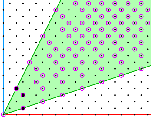
Figure 1: Key geometric objects for the matching rule $V=\{(3,1),(3,3),(2,4)\}$. (Families may consist of 1 red and 3 blue, or 3 red and 3 blue, or 4 red and 2 blue points.) Elements of $V$ are marked with filled discs. The set $\operatorname{cone}(V)$ is shaded: matchings with exponential tails are possible for intensity vectors $(\lambda_{\text{red}},\lambda_{\text{blue}})$ in its interior, while for $d\leq 2$ only a power law is possible in its boundary. The lattice $\mathcal{L}(V)$ is shown by the dots, and the matchable vectors $\mathcal{L}_{+}(V)$ (corresponding to sets of points that can be partitioned into families) are circled. Since $\mathcal{L}\neq\mathbb{Z}^{2}$, factor matchings must have infinite mean family size in $d=1$, even in the interior of the cone.

We denote by $C,c$ positive constants whose value may change from line to line. Generally statements would hold for $c$ small enough and $C$ large enough.

1.2 Charge and mass transport

As noted, the behaviours we get for matchings in general are similar to the previously studied cases of one and two colour matchings. A central new idea is to define a charge function with useful properties. We will assign each colour $i$ a real number $\eta_{i}$ called the charge. We think of charge $\eta_{i}$ as located on each point of colour $i$, and write $\eta(x)=\eta_{i}$ for $x\in[\Pi_{i}]$. We will choose $\eta$ so that the total charge in each family is non-positive. In the unsatisfiable case we can do this in such a way that the average charge over space is positive, which leads to a contradiction using the mass transport principle (see below). In the critical case the average charge is $0$, and conservation is used to derive lower bounds on the tail of the matching distances. In order to choose appropriate charges, we use hyperplane separation (see e.g. [9, Chapter 11]).

Proposition 5 (Hyperplane separation).

If $C,K\in\mathbb{R}^{n}$ are disjoint convex sets and $K$ is compact, then there exists a non-zero $\eta\in\mathbb{R}^{n}$ so that $\inf_{x\in K}(\eta\cdot x)\geq\sup_{y\in C}(\eta\cdot y)$. If $C$ is closed then the inequality is strict.

We use this for the singleton set $K=\{\lambda\}$, and $C=\operatorname{cone}(V)$. Clearly for any $\eta$ and cone $C$ we have $\sup_{y\in C}(\eta\cdot y)\in\{0,+\infty\}$; the inequality then implies that the supremum must be $0$, so that the charge in each family is non-positive.

Another important tool is the mass-transport principle, which we use in the measure-theoretic form below. For background and extensions, see [8, 2, 1]

Lemma 6 (Mass transport).

Let $\mu$ be a measure on $\mathbb{R}^{d}\times\mathbb{R}^{d}$ that is invariant under the diagonal action of translations, i.e. $\mu((A+x)\times(B+x))=\mu(A\times B)$ for any $x\in\mathbb{R}^{d}$ and any Borel sets $A,B\subset\mathbb{R}^{d}$. Then $\mu(B\times\mathbb{R}^{d})=\mu(\mathbb{R}^{d}\times B)$ for any Borel $B$.

In applications, $\mu$ is often taken to be the expectation of a diagonally invariant random measure, and then we think of $\mu(A\times B)$ as the expected amount of mass sent from $A$ to $B$. Then the mass transport principle says that the total expected mass transported out of a set equals the expected mass transported into it.

Proof.

Suppose first that $B$ is the unit cube $[0,1)^{d}$. Define a function on $\mathbb{Z}^{d}\times\mathbb{Z}^{d}$ by $f(x,y)=\mu((x+B)\times(y+B))$. Invariance of $\mu$ implies that this function is invariant under the action of $\mathbb{Z}^{d}$, and so $f(0,x)=f(-x,0)$. Summing this over $x\in\mathbb{Z}^{d}$ yields the claim for $B$ the unit cube (since all terms are non-negative, the order of summation can be changed.)

Similarly, using $B=[t,t+a)^{d}$ and summing over $x\in(a\mathbb{Z})^{d}$ we get the claim for cubes of side $a$. Unions give any open set $B$, and therefore also any Borel set $B$. ∎

Structure of the paper.

Sections 2, 3 and 5 contain proofs involving the unsatisfiable, underconstrained and critical cases respectively. Theorem 2 about factor matchings is proved in Section 4. In Section 6 we prove Theorem 3 concerning the case of infinitely many allowed family types. Section 7 contains the proof of Proposition 4 on colourful pair matchings. We end with some open questions in Section 8.

Acknowledgment.

This work was initiated during a UBC Probability Summer School, and advanced while some of the authors were visiting Microsoft Research. We are grateful to Microsoft Research for their support. OA is supported by NSERC.

2 The unsatisfiable case

Proof of Theorem 1 (i).

As with most proofs based on mass transport, the key is to find a useful mass transport function. Given an invariant matching scheme, we show how to construct a mass transport that contradicts the principle. Since $\lambda\not\in\operatorname{cone}(V)$ and $\operatorname{cone}(V)$ is closed convex set, by Proposition 5 there is a vector of charges $\eta\in\mathbb{R}^{q}$ such that $\eta\cdot\lambda>\sup\{\eta\cdot x:x\in\operatorname{cone}(V)\}$. Since $\operatorname{cone}(V)$ is a cone, this supremum is in $\{0,+\infty\}$ and thus must be $0$, and so $\eta\cdot\lambda>0$. To apply the mass transport principle, it is convenient to work with non-negative charges. To this end, we let $K=-\min_{i}\eta_{i}$. By a slight abuse of notation, we let $\eta(x)=\eta_{i}$ for any point $x\in[\Pi_{i}]$.

Suppose that ${\cal M}$ is a translation invariant $V$-matching, and recall that ${\cal M}(x)$ is the family of the matching that contains the point $x$. Define the translation invariant measure $\mu$ on $\mathbb{R}^{d}\times\mathbb{R}^{d}$ by

$$\mu(A\times B)=\mathbb{E}\sum_{x\in A\cap[\Psi]}\ \sum_{y\in{\cal M}(x)\cap B}\frac{K+\eta(x)}{\#{\cal M}(x)}.$$

This corresponds to the mass transport in which each point $x\in[\Pi_{i}]$ sends out a total mass $K+\eta_{i}$ divided evenly to its family ${\cal M}(x)$, and no mass to points outside its family. The total mass received by a point $y$ is $\sum_{x\in{\cal M}(y)}\frac{K+\eta(x)}{\#{\cal M}(y)}\leq K$, since the total $\eta$-charge in a family is non-positive.

We apply Lemma 6 to $\mu$. Let $B$ be a set of volume $1$. We have

$$\mu(\mathbb{R}^{d}\times B) =\mathbb{E}\sum_{x\in[\Psi]}\ \sum_{y\in{\cal M}(x)\cap B}\frac{K+\eta(x)}{\#{\cal M}(x)}$$

$$=\mathbb{E}\sum_{y\in[\Psi]\cap B}\sum_{x\in{\cal M}(y)}\frac{K+\eta(x)}{\#{\cal M}(x)}$$

$$\leq\sum_{i}K\lambda_{i},$$

since the inner sum on the second line is at most $K$ for any $y$. However,

$$\mu(B\times\mathbb{R}^{d}) =\mathbb{E}\sum_{x\in[\Psi]\cap B}K+\eta(x)$$

$$=\sum_{i}\lambda_{i}(K+\eta_{i})>\sum_{i}K\lambda_{i},$$

since $\eta\cdot\lambda>0$. The contradiction implies that an invariant $V$-matching does not exist. ∎

3 The underconstrained case

While the cases of Theorem 1 are split according to the tail behaviour of $X$, the proofs are separate for the cases $\lambda\in\partial(\operatorname{cone}(V))$ and $\lambda\in\operatorname{cone}(V)^{\circ}$. We begin with the latter, forming part of case (iii).

We first show the existence of an invariant matching scheme that gives the desired tail bounds for the diameter of the family of a typical point. We begin with the case of dimension $d=1$, and then use the one-dimensional case to derive the claim for general $d$.

Assume $d=1$, and consider the process $\Pi(0,t]=(\Pi_{1}(0,t],\dots,\Pi_{q}(0,t])$, taking values in $\mathbb{N}^{q}$ (for $t\geq 0$). Define also

$$T=\inf\Big{\{}t>0:\Pi(0,t]\in\mathcal{L}_{+}(V)\text{ and }\Pi(0,t]\neq 0\Big{\}},$$ (1)

i.e. the first $t$ for which the vector $\Pi(0,t]$ is matchable and non-zero. The main step in the proof is the following lemma.

Lemma 7.

Suppose $d=1$ and $\lambda\in\operatorname{cone}(V)^{\circ}$. Then $T$ as defined in (1) has an exponential tail: there exist constants $C,c>0$ such that $\mathbb{P}(T>t)<Ce^{-ct}$ for any $t>0$.

The proof consists of three steps. We show that with high probability at all large times, $\Pi(0,t]$ is “well inside” $\operatorname{cone}(V)$ in a certain sense, that $\Pi(0,t]$ visits the lattice $\mathcal{L}$ regularly, and finally that any point in $\mathcal{L}$ that is well inside the cone corresponds to a matchable set.

We begin with a simple geometric statement. Let $\|\cdot\|$ denote the Euclidean norm, and $\operatorname{dist}(x,A)$ the Euclidean distance from the point $x$ to the set $A$.

Lemma 8.

Suppose $\lambda\in\operatorname{cone}(V)^{\circ}$. Let $\delta=\frac{1}{2}\operatorname{dist}(\lambda,\operatorname{cone}(V)^{\mathrm{c}})$, and suppose $\pi\in\mathbb{R}^{q}$ satisfies $\|\pi-s\lambda\|<\delta s$ for some $s>0$, and let $\xi\in\mathbb{R}^{q}$. Then $s>\|\xi\|/\delta$ implies $\pi\in\xi+\operatorname{cone}(V)$ (the translated cone).

Proof.

We have $\|(\pi-\xi)-s\lambda\|\leq\|\xi\|+\|\pi-s\lambda\|<2\delta s$. By linearity, $2\delta s=\operatorname{dist}(s\lambda,\operatorname{cone}(V)^{c})$, hence $\pi-\xi\in\operatorname{cone}(V)$. ∎

For $\alpha>0$ let

$$\operatorname{cone}_{\alpha}(V):=\left\{\sum a^{i}{v}^{i}:a\in[\alpha,\infty)^{k}\right\}.$$

Clearly $\operatorname{cone}_{\alpha}(V)\subset\operatorname{cone}(V)$ and is just a translation of the cone, since $\operatorname{cone}_{\alpha}(V)=\operatorname{cone}(V)+\alpha\sum{v}^{i}$.

Lemma 9.

For any $V,\lambda$, satisfying $\lambda\in\operatorname{cone}(V)^{\circ}$, and any $\alpha>0$ there exist $C,c>0$ such that for any $t$,

$$\mathbb{P}\Bigl{(}\forall s>t:\Pi(0,s]\in\operatorname{cone}_{\alpha}(V)\Bigr{)}\geq 1-Ce^{-ct}$$ (2)

Proof.

Fix $\varepsilon>0$. For any given $t$ we have

$$\mathbb{P}\Big{(}|\Pi_{i}(0,t]-t\lambda_{i}|\geq\varepsilon t\Big{)}\leq Ce^{-ct},$$

where $c,C$ depend only on $\varepsilon,\lambda_{i}$. A union bound shows that

$$\mathbb{P}\Big{(}\forall\text{ integers }n>t:|\Pi_{i}(0,n]-n\lambda_{i}|<\varepsilon n\Big{)}\geq 1-Ce^{-ct},$$

where only $C$ has changed. Since $\Pi_{i}(0,s]$ is monotone in $s$, as long as $t>\lambda_{i}/\varepsilon$ it follows that

$$\mathbb{P}\Big{(}\forall s>t:|\Pi_{i}(0,s]-s\lambda_{i}|<2\varepsilon s\Big{)}\geq 1-Ce^{-ct},$$

and by changing $C$ again, this holds for all $t$. Since this holds for each of $d$ coordinates, we get

$$\mathbb{P}\Big{(}\forall s>t:\|\Pi(0,s]-s\lambda\|<2d\varepsilon s\Big{)}>1-Ce^{-ct}.$$ (3)

Apply (3) with $\varepsilon=\frac{1}{4d}\operatorname{dist}(\lambda,\operatorname{cone}(V)^{c})$, and let $\xi=\alpha\sum{v}^{i}$, so that $\operatorname{cone}_{\alpha}(V)=\xi+\operatorname{cone}(V)$. If $t>\|\xi\|/\delta$, then by Lemma 8 with exponentially high probability (in $t$), for all $s>t$ we have $\Pi(0,s]\in\operatorname{cone}_{\alpha}(V)$.

This completes the proof for $t>\|\xi\|/\delta$. By adjusting $C$ we get the result for smaller $t$. ∎

Lemma 10.

Assume $\lambda\in\operatorname{cone}(V)^{\circ}$. Then for some constants and all $t$,

$$\mathbb{P}\Big{(}\exists s\in(t,2t)\text{ such that }\Pi(0,s]\in\mathcal{L}\Big{)}>1-Ce^{-ct}.$$ (4)

Proof.

Since $\operatorname{cone}(V)$ has a non-empty interior, $V$ contains a basis for $\mathbb{R}^{q}$. (This is actually all we need to know about $\lambda$ and $V$ for this lemma.) Hence the lattice $\mathcal{L}$ has full dimension $q$, and so the quotient $\mathbb{Z}^{q}/\mathcal{L}$ is a finite group. Identifying $\Pi(0,t]$ with its coset $\Pi(0,t]+\mathcal{L}$, we see that the process $\{\Pi(0,t]\}_{t\geq 0}$ is a continuous time random walk on a finite group. It is irreducible since the possible jumps include adding a single point of any colour, and so generate $\mathbb{Z}^{q}$ and its quotients. Thus the probability of avoiding the $0$ coset for time $t$ is exponentially small. ∎

Combining Lemmas 10 and 9 we have proved:

Corollary 11.

Let $T_{\alpha}:=\min\{t\geq 0:x(t)\in\operatorname{cone}_{\alpha}(V)\cap\mathcal{L}\}$, then there are $c,C$ depending only on $V$, $\lambda$ and $\alpha$ such that $\mathbb{P}(T_{\alpha}>t)<Ce^{-ct}$.

The last ingredient for Lemma 7 is the following lemma.

Lemma 12.

Assume $\lambda\in\operatorname{cone}(V)^{\circ}$, then there exists $\alpha>0$ for which

$$\mathcal{L}\cap\operatorname{cone}_{\alpha}(V)\subset\mathcal{L}_{+}.$$

Thus if a vector can be represented as a combination of vectors of $V$ with sufficiently large coefficients, and can also be represented using integer coefficients then it can be represented using positive integer coefficients. Recall that we use superscripts for indices of family types.

Proof.

For any $\alpha$, and $x\in\mathbb{R}^{q}$, suppose $x\in\mathcal{L}\cap\operatorname{cone}_{\alpha}(v)$. Then $x=\sum n^{i}{v}^{i}$ for some integer vector $n=(n^{1},\dots,n^{k})$ and also $x=\sum a^{i}{v}^{i}$ for a vector $a$ with $\min_{i}a^{i}\geq\alpha$. In particular $\sum(a-n)^{i}{v}^{i}=0$. Thus we consider the subspace $W\subset\mathbb{R}^{k}$ of linear relations between the elements of $V$, namely $W:=\{b\in\mathbb{R}^{k}:\sum b^{i}{v}^{i}=0\}$. Let $\mathcal{L}^{*}:=W\cap\mathbb{Z}^{k}$ be the dual lattice of integer vectors in $W$. If $W=\{0\}$ then there is a unique way to write each vector $x\in\mathbb{R}^{q}$ as a linear combination of vectors in $V$ and thus $n=a$ and in particular $n^{i}\geq\alpha$. In this case the lemma holds with any $\alpha>0$. We assume therefore that $\dim W>0$.

We now show that any point in $W$ (and in particular $n-a$) is within bounded distance from $\mathcal{L}^{*}$. Since the vectors ${v}^{i}$ have integer coordinates, and since a set of integer vectors is linearly independent over the reals if and only if they are linearly independent over the rationals (or equivalently, over the integers), $\mathcal{L}^{*}$ contains a basis for $W$, which we denote $\ell_{1},\dots,\ell_{k-q}$. We now fix our $\alpha$ to be $\alpha=\sum\|\ell_{i}\|$. Any $w\in W$ we can written in this basis as $w=\sum b_{i}\ell_{i}$. Let $w^{\prime}=\sum\lfloor b_{i}\rfloor\ell_{i}$, then $w^{\prime}\in\mathcal{L}^{*}$, and $\|w-w^{\prime}\|\leq\sum\|\ell_{i}\|=\alpha$.

Apply the above to $w=a-n\in W$. Then $w^{\prime}\in W$, so $x=\sum(n+w^{\prime})^{i}{v}^{i}$ is an integer combination of the ${v}^{i}$s. Moreover, since $\|a-(n+w^{\prime})\|=\|w-w^{\prime}\|\leq\alpha$ we find $(n+w^{\prime})^{i}\geq a^{i}-\alpha\geq 0$. In particular, $x\in\mathcal{L}_{+}$. ∎

Proof of Lemma 7.

This follows from Corollaries 11 and 12. ∎

Proposition 13.

If $\lambda\in\operatorname{cone}(V)^{\circ}$ then there exists a translation invariant matching scheme on $\mathbb{R}$ such that $\mathbb{P}^{*}(X>r)<e^{-cr}$ for some $c>0$.

Roughly, we search in a greedy manner for intervals containing matchable sets of points, and partition points in each such interval to valid families in an arbitrary manner. The resulting construction depends on a starting point $0$. From this we construct a translation invariant matching by considering a stationary version of a related Markov chain.

Proof.

Consider the following continuous time Markov chain on $\mathbb{N}^{q}$. At rate $\lambda_{i}$ increase the $i$th coordinate. If the resulting state is in $\mathcal{L}_{+}$, jump immediately to $0$. This corresponds to accumulating points along $\mathbb{R}$. The state gives the number of unmatched points of each colour. As soon as it is possible to match all points yet unmatched, we match them and the state reverts to $0$.

By Lemma 7 the time to return to $0$ after leaving it has an exponential tail, and thus the Markov chain is positive recurrent, and has a stationary distribution. We now use a stationary version of this Markov chain in order to construct our matching.

If the chain moves from $v$ to $v+e_{i}$ at time $t$ then we have a point of colour $i$ at position $t$. There is a slight complication since when the chain jumps to state $0$ we might not be able to determine from the trajectory of the Markov chain what colour of point has just arrived. We could resolve this by additional randomness, but instead let us modify the state space to $\mathbb{N}^{q}\times\{1,\dots,q\}$, and use the second coordinate to record the index of the last coordinate changed. Clearly positive recurrence is maintained, and the trajectory of the Markov chain at stationarity determines a Poisson processes $\Pi_{i}$. The times $(T_{i})$ at which the chain jumps to $0\times\{1,\dots,q\}$ partition $\mathbb{R}$ in a stationary way into intervals $(T_{i},T_{i+1}]$ so that the points in each interval form a matchable set. We can now fix an arbitrary way of matching the points in each of these intervals and we are done. ∎

This concludes the proof of the upper bound for the $d=1$ case. In order to extend our analysis to $d\geq 2$, we use a dimension reduction trick. A similar trick has been used in [4]. The key is to make use of a suitable random isomorphism between the measure spaces $\mathbb{R}$ and $\mathbb{R}^{d}$ and appeal to the $d=1$ case proved above.

Lemma 14 ([4]).

There exists a random directed graph $H$ with vertex set $\mathbb{Z}^{d}$ and only nearest-neighbour edges, with the following properties.

1. $H$ is almost surely a directed bi-infinite path spanning $\mathbb{Z}^{d}$.

2. $H$ is invariant in law under translations of $\mathbb{Z}^{d}$.

3. There exists $C=C(d)\in(0,\infty)$ such that for any $x,y\in\mathbb{Z}^{d}$ we have almost surely $\|x-y\|^{d}\leq Cd_{H}(x,y)$, where $d_{H}$ denotes the graph distance along the path $H$.

For a proof, see [4, Proposition 5]. The construction there is based on taking a random translation of a $d$-dimensional Hilbert curve (see Figure 2).

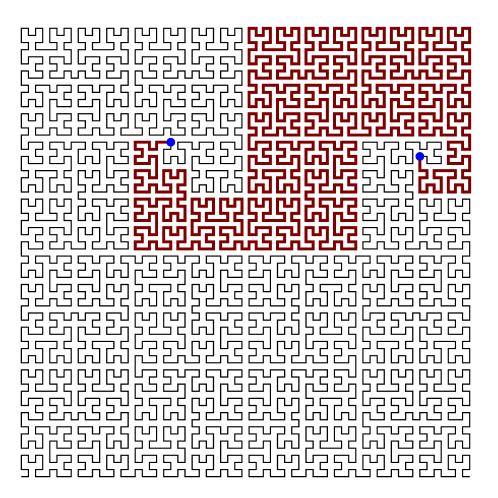
Figure 2: Part of Hilbert’s space filling curve. The number of sites visited between two given points is at least a constant times the square of the distance. A similar construction works in higher dimensions.

Lemma 15.

Let ${\cal M}$ be a translation invariant $V$-matching scheme of independent Poisson processes in $\mathbb{R}$, with typical family diameter $X$. Then for any $d>1$ there exists a translation-invariant $V$-matching scheme ${\cal M}^{\prime}$ of independent Poisson processes in $\mathbb{R}^{d}$ of the same intensities whose typical family diameter $X^{\prime}$ satisfies $\mathbb{P}(X^{\prime}>r^{d})\leq\mathbb{P}(X>cr-C)$ for all $r$, where $c,C$ are constants depending only on $d$.

Proof.

Let ${\cal M}$ be the $V$-matching of Poisson processes $(\Pi_{i})$ in $\mathbb{R}$. It suffices to find a $V$-matching ${\cal M}^{\prime}$ on $\mathbb{R}^{d}$ that is invariant in law under translations of $\mathbb{Z}^{d}$ and satisfies the claimed bound; then we obtain a fully translation invariant version by translating ${\cal M}^{\prime}$ by an independent uniform element of $[0,1]^{d}$.

Let $H$ be as in Lemma 14 and independent of ${\cal M}$. As in [4] we define a bijection $S:\mathbb{Z}\to\mathbb{Z}^{d}$ by letting $S^{-1}(x)$ be the signed graph-distance along the path $H$ from $0\in\mathbb{Z}^{d}$ to $x$ (i.e. $\pm d_{H}(0,x)$, with sign $+$ if the path $H$ is directed from $0$ to $x$, and $-$ otherwise).

Now, given the processes $\Pi_{i}$ on $\mathbb{R}$ define point processes $\Pi^{\prime}_{i}$ on $\mathbb{R}^{d}$ as follows. For each point $x\in[\Pi_{i}]$, let $x^{\prime}$ be a uniform point in the cube $S(\lfloor x\rfloor)+[0,1]^{d}$, independent of all others. Let $\Pi^{\prime}_{i}$ be the simple point process whose support is the set of resulting points $x^{\prime}$. Clearly $(\Pi^{\prime}_{i})_{i=1}^{q}$ are independent Poisson process of intensities $\lambda_{i}$ on $\mathbb{R}^{d}$. For each family $F\in[{\cal M}]$ be can define a corresponding family $F^{\prime}=\{x^{\prime}:x\in F\}$; let ${\cal M}^{\prime}$ be resulting $V$-matching. The invariance property in Lemma 14 implies that ${\cal M}^{\prime}$ is invariant in law under translations of $\mathbb{Z}^{d}$.

If a family $F\in[{\cal M}]$ has diameter $r$ in $\mathbb{R}$, then by Lemma 14(iii) $F^{\prime}$ has diameter at most $C(r+1)^{1/d}+\surd d$ in $\mathbb{R}^{d}$. The required bound follows. ∎

Remark.

It is possible to avoid the discretization to $\mathbb{Z}^{d}$ by constructing a (continuous) space filling curve $H:\mathbb{R}\to\mathbb{R}^{d}$ which is an isomorphism of measure spaces and satisfies $\|x-y\|^{d}\leq|H^{-1}(x)-H^{-1}(y)|$ for a.e. $x,y$. The construction is not very different from that of Lemma 14. If $H$ is considered only up to translation of its parameter, then it can be made translation invariant (this is analogous to taking a directed path and not a bijection from $\mathbb{Z}$ to $\mathbb{Z}^{d}$). Then we simply set $\Pi^{\prime}$ be the push-forward of $\Pi$ and ${\cal M}^{\prime}$ the push-forward of ${\cal M}$ under the diagonal action of $H$.

Proof of Theorem 1 (iii), case $\lambda\in\operatorname{cone}(V)^{\circ}$.

The upper bound is a combination of Propositions 13 and 15.

The lower bound is trivial: By our assumptions on $V$ there is at least one unit vector that is not in $V$, meaning there is at least one colour $i$ for which a single point of colour $i$ is not a legal family. The lower bound now follows from the event of a having a point of colour $i$ in the unit cube with no other points (of any colour) within radius $r$. This event has probability $ce^{-cr^{d}}$ ∎

4 Factor matchings

Here we prove Theorem 2. The proof builds on some of the ideas from the proof of Theorem 1, but additional ideas are needed. Indeed, as we shall discuss below, the construction giving the upper bound in the underconstrained case above can be seen as a special case of the construction used for Theorem 2(ii). Note that throughout this section we have $d=1$.

4.1 A lower bound

We start with the lower bound in the case $\lambda\in\operatorname{cone}(V)^{\circ}$ and $\mathcal{L}\neq\mathbb{Z}^{q}$: (clause (iii)), which is different from the exponential tail given by Theorem 1.

Lemma 16.

If $\mathcal{L}\neq\mathbb{Z}^{q}$, then any translation invariant matching that is a factor of the Poisson processes has $\mathbb{E}^{*}X=\infty$.

Proof.

Suppose for a contradiction that there is such a factor matching with $\mathbb{E}^{*}X<\infty$. For any $t\in\mathbb{R}$, let $R(t)=(R(t)_{1},\dots,R(t)_{q})$ be the vector with $R(t)_{i}$ the number of points in $[\Pi_{i}]\cap(t,\infty)$ whose family intersects $(-\infty,t]$. Note that if there is a point at $a$ which contributes to $R(0)$, then $\operatorname{diam}({\cal M}(a))\geq a$, and so (by a standard property of the Palm process, [6, eq. (5)])

$$\mathbb{E}\left[\sum_{i}R(0)_{i}\right]\leq\sum\lambda_{i}\int_{0}^{\infty}\mathbb{P}^{*}(X\geq a)da=\mathbb{E}^{*}X.$$

Thus in any matching with $\mathbb{E}^{*}X<\infty$, the coordinates of $R(0)$ are almost surely finite. Since $R(t)-R(0)$ is finite, it follows that a.s. $R(t)$ is finite for all $t$.

Next, let $Q(t)=R(t)+\Pi(0,t]$, and consider how the process $Q(t)$ evolves as $t$ is increased across a point of some colour $i$. If the point at $t$ is the minimal of its family then $R$ increases by ${v}-e_{i}$ for some ${v}\in V$, and $\Pi(0,t]$ increases by $e_{i}$, so $Q(t)$ increases by some family type. If the point at $t$ is not the minimal of its family then $Q$ has no jump at $t$. It follows that $Q(t)$ is in the same coset of $\mathbb{Z}^{d}/\mathcal{L}$ for all $t>0$, and hence $R(t)-R(0)+\Pi(0,t]\in\mathcal{L}$ for all $t$.

Consider the three cosets $(R(0)+\mathcal{L},R(t)+\mathcal{L},\Pi(0,t)+\mathcal{L})$. We claim that as $t\to\infty$ they converge jointly in distribution to a triplet $(X,Y,Z)$ of independent cosets, with $Z$ uniform on $\mathbb{Z}^{q}/\mathcal{L}$. This contradicts the identity $Z=X-Y$ above. To check the claim, note that $R(0)$ may be approximated by some function of $\Pi$ restricted to $[-A,A]$, in the sense that there is a function of the restricted process taking values in $\mathbb{Z}^{q}/\mathcal{L}$ that is equal to $R(0)+\mathcal{L}$ with high probability. Similarly $R(t)$ may be approximated by the same function applied to $\Pi$ restricted to $[t-A,t+A]$. Finally, $\Pi(0,t)$ is a sum of independent terms $\Pi(0,A)+\Pi(A,t-A)+\Pi(t-A,t)$, and the middle term is asymptotically uniform in $\mathbb{Z}^{q}/\mathcal{L}$. ∎

4.2 Exponential tail

When $\mathcal{L}=\mathbb{Z}^{q}$, the last argument does not give any barrier to existence of a matching with a thinner tail, and indeed such matchings exist. We now adapt the construction from Section 3 to construct a factor matching. To demonstrate that another idea is needed, consider a particular case of Example 7: points of a single colour, where families consist of either two or three points. If (starting from some point) we wait for a matchable set and match it, then we get a partition of the points of $\Pi$ into consecutive pairs. Given $\Pi$, there are two such matchings. The construction above gives a random one of these, clearly not a factor of $\Pi$. Indeed, Theorem 2(iii) shows that any factor matching with exponential tail for $X$ must incorporate both family types.

The new idea is as follows. Suppose first that each point of $[\Pi]$ is given an independent fair coin toss. Modify the construction above so that a pair is matched if the coin of the right point is heads, while if the coin is tails then the next point of $[\Pi]$ is added to form a triplet. It is not hard to show that if this procedure is applied to the points of $(T,\infty)$ then the resulting matchings converge as $T\to-\infty$, and the limit is a factor of $\Pi$ together with the coins. Clearly we cannot define these coins as a factor of $\Pi$ while keeping them independent of $\Pi$. However, in the construction below we assign a coin to each point of $\Pi$ as a factor of $\Pi$, by looking at the distances to the previous point of $[\Pi]$, so that the resulting coins are i.i.d. and independent of the colours.

To make this construction of a factor matching precise in the general case, we first consider integer indexed processes. Without loss of generality we may normalize $\lambda$ to have $\sum\lambda_{i}=1$. Consider a doubly infinite i.i.d. sequence of colours $(\xi_{i})_{i\in\mathbb{Z}}$ with distribution given by $\lambda$. Consider also an independent sequence of i.i.d. Bernoulli(1/2) random variables $(\epsilon_{i})_{i\in\mathbb{Z}}$.

We define the population count in an interval $I\subset\mathbb{Z}$ as the vector $\Pi(I)$ with $\Pi(I)_{i}=\#\{t\in I:\xi_{t}=i\}$. Define the good block starting at $s\in\mathbb{Z}$ to be the interval $(s,t]$ where $t>s$ is minimal such that $\epsilon_{t}=1$ and $\Pi(s,t]\in\mathcal{L}_{+}$, that is the points in $(s,t]$ are matchable and the extra variable at $t$ is $1$.

Lemma 17.

With the above notations, there are constants $c,C$ so that for any $s\in\mathbb{Z}$, if $(s,t]$ is the (unique) good block starting at $s$, then we have that $\mathbb{P}(t-s>x)<Ce^{-cx}$.

Proof.

This is essentially the same as Lemma 7, and an analogous argument works. There are two differences: points are indexed by $\mathbb{Z}$, and we require $\epsilon_{t}=1$. As in Lemma 9, with high probability $\Pi(s,t]\in\operatorname{cone}_{\alpha}$ for all large enough $t$, and by Lemma 12 we find $\Pi(s,t]\in\mathcal{L}_{+}$ for all large $t$. Since $\epsilon_{t}=1$ with probability $1/2$ for each $t$, the good block from $s$ has exponential tail. ∎

Corollary 18.

Almost surely there are only finitely many good blocks $(s,t]$ containing 0.

Proof.

This follows from Lemma 17 and the Borel-Cantelli Lemma. ∎

We now consider partitions of $\mathbb{Z}$ into good blocks. Such a partition arises from a doubly infinite sequence $(t_{i})_{i\in\mathbb{Z}}$ such that $(t_{i},t_{i+1}]$ are all good blocks. (Two such sequences are considered equivalent if they differ only in a shift of the indices.) Given such a partition we can define a matching of the points by taking some arbitrary matching of the points in each good block. We say that the sequence $(t_{i})$ is a factor of the sequences $\xi,\epsilon$ if the indicator of the set $\{t_{i}\}_{i\in\mathbb{Z}}$ is a factor. In that case, so is the resulting matching. The following is a key step towards proving Theorem 2(ii).

Proposition 19.

Almost surely, there is a unique partition of $\mathbb{Z}$ into good blocks.

Towards proving Proposition 19, we will define a Markov chain $(Z_{n})$ with state space $\mathbb{N}^{q}$. The state $Z_{n}$ will be a deterministic function of the previous state $Z_{n-1}$ together with $\xi_{n}$ and $\epsilon_{n}$. Given $Z_{n-1}$, first increase by 1 the $\xi_{n}$ coordinate to give $Z^{\prime}_{n}:=Z_{n-1}+e_{\xi_{n}}$. The next state $Z_{n}$ is equal to $Z_{n}^{\prime}$ unless $Z_{n}^{\prime}$ is a matchable vector and $\epsilon_{n}=1$, in which case we instead set $Z_{n}=0$. With the given distribution for $\xi$ and $\epsilon$, this defines a Markov transition matrix, but apriori there could be multiple sequences $(Z_{n})$ consistent with a given sequence $(\xi_{n},\epsilon_{n})$.

Subsequently, we shall deduce from Proposition 19 that there is in fact a unique process $(Z_{n})$, which moreover is a factor of $(\xi_{n},\epsilon_{n})$.

Lemma 20.

The transition matrix on $\mathbb{N}^{q}$ defined above is irreducible, aperiodic and positive recurrent.

Proof.

If $x\leq y$ coordinate-wise then $y$ is reachable from $x$, since we could have $\epsilon_{i}=0$ for as long as needed. For every state $x$ there is a matchable state $y\geq x$ coordinate-wise. By having only the last $\epsilon=1$, we see that $0$ is reachable from $x$. Thus the chain is irreducible. Since $\mathcal{L}=\mathbb{Z}^{q}$, there are matchable states $y$ of any large enough $\|y\|_{1}$, so the possible return times to $0$ have greatest common divisor $1$. Finally, if $Z_{0}=0$ then the return time to $0$ is the $t$ such that $(0,t]$ is a good block. Since this has an exponential tail, the chain is positive recurrent. ∎

Lemma 21.

Let $(Z_{n})_{n\in\mathbb{N}}$ and $(Y_{n})_{n\in\mathbb{N}}$ be two instances of the Markov chain with different initial condition $Z_{0}\neq Y_{0}$ and using the same colours $(\xi_{n})$ and coins $(\epsilon_{n})$. Then almost surely the chains agree eventually.

Proof.

By Lemma 20 and the ergodic theorem there is some $M$ such that the set $\{n:\|Z_{n}\|_{1}\leq M\}$ has density at least $2/3$. The same holds for $Y$, and therefore there are a.s. infinitely many times when $\|Z_{n}\|_{1},\|Y_{n}\|_{1}\leq M$. We shall show that each time this happens, there is some probability of coupling within some bounded time. By the Markov property, the chains almost surely couple eventually.

From any such states $(Z,Y)$, there is some positive probability that the next jump to $0$ of $Z$ and $Y$ is at the same time, after which $Z$ and $Y$ agree. To see this, note that $\mathcal{L}=\mathbb{Z}^{q}$ implies that there is a sequence of colours that, when added to $Z$ and $Y$, will make both matchable. If subsequent $\xi$’s are such a sequence with all $\epsilon_{i}=0$ except for the last, then $Z$ and $Y$ jump to $0$ together, as desired. ∎

Proof of Proposition 19.

Suppose for a contradiction that there are multiple distinct partitions of $\mathbb{Z}$ into good blocks. Each such partition gives rise to a copy $(Z_{n})$ of the Markov chain with $Z_{n}=0$ precisely at the the ends of the blocks of the partition. By Corollary 18 there are only finitely many different good blocks containing $0$, and so only finitely many different values for the Markov chains at time $0$. By Lemma 21, the associated Markov chains all agree from some time on. Thus there is some minimal $M\in\mathbb{Z}$ such that all partitions give the same value of $Z_{M}$ (and thus the chains also agree for all $n\geq M$). This $M$ is a translation invariant factor of the sequences $\xi,\epsilon$, which is impossible.

To prove existence, note that the sequence of triplets $(\xi_{n},\varepsilon_{n},Z_{n})$ is also a positive recurrent Markov chain. Take a stationary doubly infinite sequence of triplets, and note that the sequences $(\xi_{n})$ and $(\varepsilon_{n})$ are i.i.d. with marginal laws $\lambda$ and Bernoulli(1/2). Thus there is a coupling of the sequences $\xi$, $\epsilon$, and $Z$ with the given marginals. The set of times when $Z_{t}=0$ gives the endpoints of a partition to good blocks. ∎

Proof of Theorem 2(ii).

Assume without loss of generality that $\sum\lambda_{i}=1$. Consider the Palm process of the Poison process $\Pi$, with law $\mathbb{P}^{*}$. First, we construct the process $(\xi_{n},\epsilon_{n})$ from $\Pi$. Index the points of $\Pi$ by $\mathbb{Z}$ in order, with the point at $0$ having index $0$. Let $\xi_{n}$ be the colour of the $n$th point, and let $\epsilon_{n}$ be $1$ if the distance from the $n$th point to the previous one is at least $\log 2$. This constructs on the probability space of $\Pi$ the i.i.d. sequence of colours $\xi$ and the independent collection of variables $\epsilon$.

By Proposition 19 there is a unique realization of the Markov chain $Z_{n}$ driven by $\xi$ and $\epsilon$. As noted above, this gives a matching as a factor of the discretized process. Since points of $\Pi$ naturally correspond to $\mathbb{Z}$, this also gives a matching as a factor of $\Pi$.

It remains to see that in this matching, $X$ has an exponential tail. If the family of the point at $0$ contains a point greater than $t$, then either $[0,t]$ contains less than $t/2$ points, or else the good block of $0$ contains at least $t/2$ points. Both of these events have exponentially decaying probabilities in $t$, since $\sum\lambda_{i}=1$. ∎

We remark that it is also possible to define a continuous time version of the Markov chain in this section, and use the continuous process to define the factor matching (taking into account the time since the last event, which encodes the $\epsilon_{i}$). However, the discretization makes the process easier to define, and is also useful for formalizing the constructions in the next section.

4.3 Factor matching construction when $\mathcal{L}\neq\mathbb{Z}^{q}$

We now extend the ideas from the previous section to construct a factor matching for the general underconstrained case. Define the quotient group $\Gamma:=\mathbb{Z}^{q}/\mathcal{L}$, and note that since $\operatorname{cone}(V)^{\circ}$ is non-empty, $\mathcal{L}$ has full rank, and so $\Gamma$ is a finite group with canonical homomorphism from $\mathbb{Z}^{q}$.

Suppose $\mathcal{L}\neq\mathbb{Z}^{q}$, so that $|\Gamma|>1$. The reason that the construction of the previous section fails is that Proposition 19 does not hold. Indeed there are precisely $|\Gamma|$ partitions of $\mathbb{Z}$ into good blocks, and no way to select one as a factor of $\Pi$ (this can be proved similarly to Lemma 16). We introduce two key ideas in order to overcome this difficulty, at the expense of a worse tail for $X$. First, we modify the Markov chain so that a version of Lemma 21 holds (and hence also a version of Proposition 19). This is done by leaving some points unmatched, chosen independently of their colours. Second, we iterate the procedure to deal with unmatched points. Thus we have an infinite series of stages, each dealing with the increasingly spread out left-overs from the previous stages. The final product of this argument is the following.

Proposition 22.

If $\lambda\in\operatorname{cone}(V)^{\circ}$, then there exists a translation invariant matching that is a factor of the Poisson processes with $\mathbb{P}^{*}(X>t)\leq C/t$ for some constant $C$.

Proof of Theorem 2(iii).

The last proposition proves the upper bound, while the lower bound is given by Lemma 16. ∎

Overview of the construction.

The matching will be constructed in stages. In each stage we shall construct a partial matching, which consists of valid families but leaves some points unmatched. In each stage the partial matching is constructed using a variation of the Markov chain that we describe below. The diameter of families will have exponential tail. Unmatched points will be matched in some later stage. The probability that a point is matched at stage $s$ will decay exponentially in $s$. However, points at stage $s$ will typically be far apart. It will turn out that the dominant contribution to $\mathbb{P}^{*}(X>t)$ will come from $s$ with $2^{s}\approx t$.

Modified Markov chain.

Recall the Markov chain $(Z_{n})$ from the previous section, taking values in $\mathbb{N}^{q}$, with steps defined in terms of colours $\xi_{n}$ and coins $\epsilon_{n}$, which at step $n$ increases the $\xi_{n}$th coordinate, and possibly jumps to $0$.

We modify this in two ways to define a new process $Z_{n}$. First, we allow an extra value $\xi_{n}=\emptyset$, signifying that $n$ is “unoccupied”. In that case set $Z_{n}=Z_{n-1}$. The set of occupied times can have correlations, so $Z_{n}$ is no longer a Markov chain, but is still a time change of a Markov chain.

Let $Y_{n}\in\Gamma$ be the coset containing $Z_{n}$. Note that $Y_{n}$ is determined by $Y_{n-1}$ and $\xi_{n}$, with no need to know $\epsilon_{n}$, since the jumps of $Z_{n}$ to $0$ do not show in $Y_{n}$. Moreover, if we take two copies of this chain driven by the same sequence $\xi$, started at $Z_{0}$ and $Z^{\prime}_{0}$, then the coset $Y^{\prime}_{n}-Y_{n}$ does not depand on $n$. If $Y^{\prime}_{0}\neq Y_{0}$ then the two Markov chains do not couple.

The second modification is in terms of a third sequence $\zeta$, in addition to $\xi$ and $\epsilon$. We make the following assumptions about their distribution.

• $\xi_{n}$ takes values in $\{\emptyset,1,\dots,q\}$. The set $S=\{n:\xi_{n}\neq\emptyset\}$ (for support) is non-empty, and its indicator is an ergodic process.

• Conditioned on $S$, the $\xi|_{S}$ are i.i.d. with law $\lambda$.

• Conditioned on $S$, the restrictions $\epsilon|_{S}$ and $\zeta|_{S}$ take independent uniform values in $\{0,1\}$, and are also independent of $\xi$.

The $\zeta$ variables indicate some points which might be left unmatched (where $\zeta_{n}=0$).

Given the sequences $\xi,\epsilon,\zeta$, we now define the transitions of the process $Z$ and its coset process $Y$ using the following procedure. This process will be a single stage in an iterative approach, and is depicted in Figure 3. Suppose $Z_{n-1}$ is given.

• If $\xi_{n}=\emptyset$ then set $Z_{n}=Z_{n-1}$.

• If $Y_{n-1}=0$ and $\zeta_{n}=0$, then also $Z_{n}=Z_{n-1}$. In this case we say a point at $n$ is skipped.

• Otherwise, let $Z^{\prime}_{n}=Z_{n}+e_{\xi_{n}}$ (if we reach this case, $\xi_{n}\neq\emptyset$).

• If $Z^{\prime}_{n}\in\mathcal{L}_{+}$ (i.e. is matchable) and $\epsilon_{n}=1$ then $Z_{n}=0$. Otherwise, $Z_{n}=Z^{\prime}_{n}$.

Figure 3: A stage in the iterative construction of a factor matching. This flowchart shows how to compute $(Z_{n})_{n\geq a}$ given $Z_{a}$ and the sequences $\xi,\epsilon,zeta$. Proposition 26 implies that there is a unique choice of the entire sequence $(Z_{n})_{n\in\mathbb{Z}}$ consistent with the recursion.

Some observations should be made at this time. First, since the $\xi$ are not assumed to be i.i.d., the resulting processes $(Z_{n})$, $(Y_{n})$ are not Markov chains. Instead, these are time changed Markov chains which make a step at times $n\in S$. Second, $Y_{n}$ can be determined from $Y_{n-1}$, $\xi_{n}$ and $\zeta_{n}$, since we always have $Z_{n}-Z^{\prime}_{n}\in\mathcal{L}$. Thus $(Y_{n})$ is itself a (time changed) Markov chain. Finally, let $\widehat{S}$ be the set of times at which a point is skipped. Then the indicator of $\widehat{S}$ is also ergodic. (It follows from Proposition 26 below that $\widehat{S}$ is a factor of $\xi$ and $\zeta$.) Moreover, for $n\in\widehat{S}$, the procedure above does not observe $\xi_{n}$. Consequently, conditioned on $\widehat{S}$, the restriction $\xi|_{\widehat{S}}$ is an i.i.d. process with law $\lambda$.

The first steps in analysis of the process are just as in the case $\mathcal{L}=\mathbb{Z}^{q}$. While $Z_{n}$ and $Y_{n}$ are not Markov chain, their transitions at times $n\in S$ are Markovian. Consider the transition probabilities of $Z_{n}$ and $Y_{n}$ at a time $n\in S$, i.e. with $\xi_{n}$ with law $\lambda$ and independent $\epsilon_{n}$,$\zeta_{n}$.

First, we control the return times to $0$ of $Z_{n}$, in terms of the number of points in $S$.

Lemma 23.

Let $T$ be the return time to $0$ for $(Z_{n})$, started at $Z_{0}=0$ and $L_{t}=|S\cap(0,t]|$. Then for some $c,C>0$ depending only on $V$ and $\lambda$ we have $\mathbb{P}(L_{T}>n)\leq Ce^{-cn}$.

Proof.

This is proved by the exact same argument as Lemma 17: With high probaility, once $L_{n}$ is large we have $Z_{n}\in\operatorname{cone}_{\alpha}(V)$. A positive fraction of the time it is in $\mathcal{L}$ and hence also in $\mathcal{L}_{+}$. Once $Z^{\prime}_{n}\in\mathcal{L}_{+}$ and $\epsilon_{n}=1$ the process jumps to $0$. ∎

As before, if we set $Z_{s}=0$, and let $t$ be the next time at which $Z_{t}=0$, we call $(s,t]$ a good block. Thus the number of points of $S$ in the good block starting at $s\in S$ has exponential tail.

Corollary 24.

For some $C,c>0$, the probability that there is some good block $(a,b]$ containing $0$ and at least $n$ points of $S$ is at most $Ce^{-cn}$.

Proof.

There is a unique good block starting at each point of $S$. For the $n$ points just to the left of $0$, the probability that the corresponding block contains $0$ is at most $Ce^{-cn}$ by the previous lemma. For blocks starting further to the left, the probability of containing $0$ decays exponentially, and the result follows by a union bound. ∎

We now deduce that the Markov chains are well behaved.

Lemma 25.

The transition probabilities of $(Z_{n})$ and $(Y_{n})$ define irreducible, and positive recurrent Markov chains.

Proof.

For $n\in S$, we have $Y_{n}=Y_{n-1}+e_{\xi_{n}}$ unless $Y_{n-1}=0$ and $\zeta_{n}=0$, which gives an irreducible Markov chain. Since it is possible for the chain $Z_{n}$ to reach $0$ from any state, and reach any state from $0$, it is also irreducible. As in Lemma 20, the return times to $0$ have exponential tail, hence $Z_{n}$ is positive recurrent. ∎

Proposition 26.

Almost surely, there is a unique partition of $\mathbb{Z}$ into good blocks. Moreover, there are unique doubly infinite processes $(Z_{n})_{n\in\mathbb{Z}}$, $(Y_{n})_{n\in\mathbb{Z}}$ consistent with the sequences $\xi$, $\varepsilon$ and $\zeta$.

Proof.

As in the proof of Lemma 21, starting $Z$ and $Z^{\prime}$ at any two initial states and running them using the same sequences $(\xi_{n})$, $(\epsilon_{n})$, $(\zeta_{n})$, we have that $Z_{n}=Z^{\prime}_{n}$ from some time on. The proof of Proposition 19 now applies. ∎

Partial matchings.

For a process $(\xi_{n})$ taking values in $\{\emptyset,1,\dots,q\}$, a partial matching is a translation equivariant partition of some subset of $\{n:\xi_{n}\neq\emptyset\}$ into finite sets so that the values of $\xi$ in each set are a valid family type, with some points possibly left unmatched. This may be defined formally similarly to matchings of Poisson processes, and we omit a detailed definition. Given a partial matching, we let $X$ denote the diameter of the family of $0$ if $0$ is matched, and set $Z=0$ if $\xi_{0}=\emptyset$ or if $0$ is unmatched. Given a partition of $S=\{n:\xi_{n}\neq\emptyset\}$ into skipped points and good blocks, there is a partial matching of the unskipped points with families contained in good blocks.

Let $\widehat{S}$ denote the sets of $n$ such that a point at $n$ is skipped. For sequences $\xi,\epsilon,\zeta$ satisfying assumptions (A1)–(A3), the process $1_{\widehat{S}}$ is ergodic, and has intensity $\alpha$ times the intensity of $\xi$, for some $\alpha<1/2$. (It is not hard to find $\alpha=(1+|\Gamma|)^{-1}$ by analyzing the Markov chain $Y$.)

Discretization.

Having analyzed the modified Markov chains, we are now ready to continue constructing our factor matching. We first move to a discretized version of the Poisson process $\Pi$. We will then introduce partial matchings and use the discrete process to construct iteratively our factor matching. We conclude the proof by analyzing the tail of $X$ for the resulting matching.

Assume again that $\sum\lambda_{i}=1$. We replace the Poisson process by a discretized version with some additional random variables reserved for later use. Label the points of $\Pi$ by the integers $\mathbb{Z}$ in order, with the maximal point in $(-\infty,0]$ having label $0$. (Under $\mathbb{P}^{*}$ this point is at $0$.) Let $T_{n}$ be the location of point $n$, so that $T_{0}\leq 0<T_{1}$ and the gaps $T_{n}-T_{n-1}$ for $n\neq 1$ are i.i.d. $\operatorname{Exp}(1)$ random variables. Under $\mathbb{P}^{*}$, the gap $T_{1}-T_{0}$ is no different, though under $\mathbb{P}$ it is biased by its size. We now create a discrete process $\hat{\Pi}$, by rounding each gap up to an integer, i.e., define the new locations of points by $\hat{T}_{0}=\lceil T_{0}\rceil$ and $\hat{T}_{n}-\hat{T}_{n-1}=\lceil T_{n}-T_{n-1}\rceil$ for $n\in\mathbb{Z}$. Let $\hat{\Pi}=(\hat{\Pi}_{1},\dots,\hat{\Pi}_{q})$, where $\hat{\Pi}_{i}$ is the resulting process of points of colour $i$ supported within $\mathbb{Z}$.

Note that if $X=\operatorname{Exp}(1)$ then $\lceil X\rceil$ is a geometric random variable, and therefore the gaps in $\hat{\Pi}$ are geometric. Moreover, $-\lceil T_{0}\rceil=\lfloor-T_{0}\rfloor\stackrel{{\scriptstyle d}}{{=}}\lceil X\rceil-1$, so that $\hat{T}_{1}-\hat{T}_{0}\stackrel{{\scriptstyle d}}{{=}}\lceil X\rceil+\lceil X^{\prime}\rceil-1$ is a size biased geometric. It follows that every point is present in $[\hat{\Pi}]$ independently with the same probability (which happens to be $1-1/e$), except that $0\in[\hat{\Pi}]$ almost surely.

Observe that the fractional part of an exponential is independent of its integer part. For each $n\in[\hat{\Pi}]$ let $U_{\hat{T}_{n}}$ be the fractional part of $T_{n}-T_{n-1}$. Conditioned on $\hat{\Pi}$, the $(U_{n})_{n\in[\hat{\Pi}]}$ are i.i.d.. Thus we have constructed a coloured Bernoulli process on $\mathbb{Z}$, where each occupied point is also assigned some independent continuous random variable. These variables can be used for making random choices associated with $n$ as a function of the original process $\Pi$.

Iterative matching.

We are ready now to describe the complete construction of the factor matching. The procedure we describe will have an infinite sequence of stages. At each stage $s$ there will be sequences $\xi^{(s)}$, $\epsilon^{(s)}$ and $\zeta^{(s)}$ as above. The Bernoulli variables $\epsilon^{(s)}_{n}$ and $\zeta^{(s)}_{n}$ will be functions of $U_{n}$. The sequences $\xi^{(s)}$ are more delicate.

The set $S_{s}$ defined below will be equal to the set $\{n:\xi^{(s)}_{n}\neq\emptyset\}$. These sequences will satisfy assumptions (A1)–(A3), and so Proposition 26 applies, and there is a unique partition of $\mathbb{Z}$ into good blocks. Each block contains a matchable set of points and some skipped points. The sequences $\xi^{(s)}$ will be defined inductively. If $n$ has been matched in some stage prior to $s$ then $\xi^{(s)}_{n}=\emptyset$. However, we sometimes set $\xi^{(s)}_{n}=\emptyset$ also for unmatched points, in order to reserve a point for later stages.

For each $n\in[\widehat{\Pi}]$, from $U_{n}$ we define a $\operatorname{Geom}(1/2)$ variable $(G_{n})_{n\in\widehat{\Pi}}$, as well as sequences of i.i.d. Bernoullis $(\epsilon_{n}^{(s)})_{s\in\mathbb{N}}$ and $(\zeta_{n}^{(s)})_{s\in\mathbb{N}}$. We now define the sets $S_{s}$ inductively as follows. The set $S_{s}$ consists of all $n$ that were skipped at stage $s-1$, as well as all points with $G_{n}=s$. Note that there is no stage $0$, so no points are skipped at stage $0$.

More precisely, we define $S_{s}$ inductively: At stage $1$ we have $S_{1}=\{n:G_{n}=1\}$. At each stage we define

$$\xi^{(s)}_{n}=\begin{cases}\emptyset&n\notin S_{s},\\ i&n\in S_{s},n\in\hat{\Pi}_{i}.\end{cases}$$

We generate a partial matching using $\xi^{(s)}$, $\epsilon^{(s)}$ and $\zeta^{(s)}$. We denote by $\widehat{S}_{s}\cup\{n:G_{n}=s+1\}$ (see Figure 4). Thus $n\in S_{s}$ if $G_{n}\leq s$ and $n$ has not been matched in any previous stage. If $n\in S_{s}$ then we say that $n$ is active at stage $s$.

Figure 4: The iterations in the construction of the factor matching. Here ”STAGE” refers to defining a partial matching on points in $S_{s}$, and setting $\widehat{S}_{s}$ to be the set of skipped points.

Family size distribution.

We are finally able to complete our proof of Theorem 2(iii).

Proof of Theorem 2(iii).

The lower bound is given by Lemma 16. For the upper bound, we analyze the sequential matching procedure described above. First, note that for any $n\in\hat{\Pi}$ there is a.s. some $s\geq G_{n}$ with $\zeta^{(s)}_{n}=1$, so a point at $n$ is a.s. matched at some stage, and the iterative procedure indeed yields a factor matching. It remains to estimate the tail of $X$ under $\mathbb{P}^{*}$.

Recall that under $\mathbb{P}^{*}$, there is a point at $0$, and let $\hat{X}$ be the diameter of its family in the discrete process. Points of $\hat{\Pi}$ are in natural correspondence with points of $\Pi$, and distances in $\hat{\Pi}$ are larger, so deterministically $X\leq\hat{X}$. Note that $\hat{\Pi}$ is not ergodic since there is always a point at $0$. However, it is an ergodic process conditioned to have a point at $0$. Since this condition has positive probability for the discrete process, any almost sure statement about the ergodic process applies also to $\hat{\Pi}$, and any bound on a probability holds with a constant factor. We therefore consider from now on a process where there is a point at $0$ with the same probability as any other $n$.

The idea for bounding the probability that $\hat{X}$ is large, is that one of several things must happen. Either $0$ is matched at a late stage, or else the good block containing $0$ at an early stage $s$ is atypically large. In the latter case, either there are many active points in the good block, or there are unusually few. We show that all of these are unlikely.

Let us consider the process $1_{S_{s}}$ of points which are active at stage $s$. This is an ergodic process, and our first task is to compute its intensity, denoted $\beta_{s}$. Let $\gamma$ be the intensity of $\hat{\Pi}$ (which happens to be $(1-1/e)$, though the value is not important to us). Then $\beta_{1}=\gamma/2$, as these are the points of $\hat{\Pi}$ with $G_{n}=1$. Each point of $S_{s}$ is skipped, and so in $\hat{S}_{s}$ with probability $\alpha$, so recursively, $\beta_{s}=\alpha\beta_{s-1}+2^{-s}\gamma$, with $2^{-s}\gamma$ being the intensity of points of $\hat{\Pi}$ with $G_{n}=s$. This leads to $\beta_{s}=\frac{\gamma}{1/2-\alpha}(2^{-s}-\alpha^{s})\leq C2^{-n}$ for some universal constant $C$. (Recall that $\alpha<1/2$.)

Fix some $t$. We split the event $\hat{X}>t$ according to the stage at which $0$ is matched. If this stage is $s$, then necessarily $0\in S_{s}$. Let $I\subset\mathbb{Z}$ be the good block in stage $s$ containing $0$. We have

$$\mathbb{P}^{*}\big{(}X\geq t\big{)}\leq\mathbb{P}^{*}\big{(}\hat{X}\geq t\big{)}\leq\sum_{s}\mathbb{P}^{*}\big{(}0\in S_{s},|I|\geq t\big{)}$$

Now for any $s$ we have $\mathbb{P}^{*}(0\in S_{s})=\beta_{s}/\gamma\leq(C/\gamma)2^{-s}$ (the factor of $1/\gamma$ is since $\mathbb{P}^{*}$-almost surely $0\in\hat{\Pi}$). Thus the contribution to the above sum from $s$ with $2^{s}>t$ is at most $\frac{2C}{\gamma t}$. Let us focus on $\mathbb{P}^{*}(0\in S_{s},|I|\geq t)$ for smaller $s$.

For some $\delta>0$ to be specified below, let $B_{s}=\{|S_{s}\cap I|>\delta\beta_{s}t\}$ be the event that $I$ contains many points of $S_{s}$. By Corollary 24, $\mathbb{P}(B_{s}|0\in S_{s})\leq C_{1}e^{-c_{2}\delta\beta_{s}t}$ for some constants.

Let $D_{s}$ be the event that at least one of $(0,t/2]$ and $[-t/2,0)$ contains at most $\delta\beta_{s}t$ points of $S_{s}$. The set $S_{s}$ includes all $n$ with $G_{n}=s$, which is a Bernoulli percolation with intensity $2^{-s}\gamma$. Thus the number of points of $S_{s}$ in an interval $J$ dominates a binomial $\operatorname{Bin}(|J|,2^{-s}\gamma)$. We fix $\delta$ so that $2^{-s}\gamma t/2>2\delta\beta_{s}t$, i.e. the binomial gives in expectation twice as many points as are allowed on the event $D_{s}$. By a standard large deviation estimate for binomials, $\mathbb{P}(D_{s}|0\in S_{s})\leq C_{3}e^{-c_{4}\beta_{s}t}$.

Observe that $0\in S_{s}\cap\{|I|\geq t\}$ implies $B_{s}\cup D_{s}$, and therefore

$$\mathbb{P}(0\in S_{s}\cap\{|I|\geq t\}) \leq\mathbb{P}(0\in S_{s})\left[\mathbb{P}(B_{s}|0\in S_{s})+\mathbb{P}(D_{s}|0\in S_{s})\right]$$

$$\leq(C/\gamma)2^{-s}\left[C_{1}e^{-c_{2}\delta\beta_{s}t}+C_{3}e^{-c_{4}\beta_{s}t}\right]$$

$$\leq C_{5}2^{-s}e^{-c_{6}t/2^{s}}.$$

It is easy to verify that summing this over $s$ with $2^{s}\leq t$ gives a total of order $1/t$. ∎

5 The critical case

To complete the proofs of Theorems 1 and 2, we turn to the critical case. As noted above, the simplest example of this case is matching points of two Poisson processes of equal densities. In this case the upper and lower bounds were proved in [6] (in all dimensions). Our proof of the lower bound follows a similar argument to the one in [6]. To prove the upper bound, we reduce the general critical case to the two colour case. The upper bound of Theorem 1(ii), as well as Theorem 2(i) both follow from the construction in Lemma 27.

5.1 Upper bound: constructing a matching

Lemma 27.

With the notations of Theorem 1, suppose $\lambda\in\partial(\operatorname{cone}(V))$. Then for some $C$, there exists a translation-invariant $V$-matching scheme such that for all $r$

$$\mathbb{P}^{*}(X>r)\leq\begin{cases}Cr^{-d/2}&d\leq 2,\\ e^{-Cr^{d}}&d>2.\end{cases}$$

Proof.

Our starting point is [6, Theorem 1] which shows that there exists a two-colour matching between equal intensity Poisson process with the desired tail bounds. In our notations, this is the case $q=2$, with $\lambda_{1}=\lambda_{2}$ and $V=\{(1,1)\}$. We proceed to generalize this in several steps.

The next case we consider is $V=\{(1,1,\dots,1)\}$, i.e. there is just one family type, consisting of one point of each colour. Since $\lambda\in\operatorname{cone}(V)$, all the Poisson processes must have the same intensity, which without loss of generality we may assume is $1$. To construct the required matching, start with a Poisson process with unit intensity $\Pi_{1}$. The two-colour matching conditioned on $\Pi_{1}$ gives a law for a second Poisson process together with a matching between its points and those of $\Pi_{1}$. Take $q-1$ independent samples from this conditional law. Together with $\Pi_{1}$ we now have $q$ independent Poisson processes as well as matchings between $\Pi_{1}$ and each of the others. This gives a natural partition of the points of all $q$ Poisson processes into valid families. Since there are only finitely many colours, up to constants this matching scheme has the same tail behaviour as the two-colour scheme: $\mathbb{P}^{*}(X>r)\leq(q-1)\mathbb{P}^{*}(X^{\prime}>r/2)$, where $X^{\prime}$ is the distance in the two-colour matching.

The next step is the case $V=\{{v}\}$, where there is just a single family type. Note that necessarily $\lambda=a{v}$ for some $a>0$. To construct the matching, let $q^{\prime}=\sum{v}^{i}$, and start with a $q^{\prime}$-colour matching where all colours have intensity $a$ and all families have type $(1,1,\dots,1)$. Such a matching scheme exists by the previous paragraph. Next, partition the $q^{\prime}$ colours into $q$ classes, with ${v}^{i}$ colours in the $i$th class. Let $\Pi_{i}$ be the sum of the Poisson processes of colours in the $i$th class. Clearly taking the resulting Poisson processes with the same partition to families yields the resulting matching scheme, with the same distribution for $X$.

Finally we consider the general case. Since $\lambda\in\operatorname{cone}(V)$, we can write $\lambda=\sum_{j=1}^{k}a^{j}{v}^{j}$ for some non-negative coefficients $a^{j}$. For each $j$, consider an independent matching scheme ${\cal M}_{j}$ as above with a single family type ${v}^{j}$, of Poisson processes $\{\Pi_{i,j}\}_{i\leq q}$ with intensities given by the vector $a^{j}{v}^{j}$. Let ${\cal M}=\sum_{j}{\cal M}_{j}$ and $\Pi_{i}=\sum_{j}\Pi_{i,j}$. Then ${\cal M}$ is a valid matching scheme of Poisson processes with intensities given by $\lambda$. Finally, $\mathbb{P}^{*}(X>r)\leq\max_{j}\mathbb{P}^{*}(Z_{j}>r)$ has the required tail. ∎

Lemma 28.

If $d=1$ and $\lambda\in\partial\operatorname{cone}(V)$, there is a factor matching with $\mathbb{P}^{*}(X>t)\leq C/\surd{t}$.

To prove this, we adopt the proof of Lemma 27, together with some ideas from the proof of Theorem 2.

Proof.

First, note first that the matching in [6] in the one dimensional two colour case is a factor. (Recall, this matching recursively matches a red point to a blue point immediately to its right and removes the pair.) This has the required tail. This matching is also valid for a discretized process with points on a subset of $\mathbb{Z}$, and has the same tail for $X$.

As above, we can write $\lambda=\sum a^{j}v^{j}$. We would like to split the process $\Pi_{i}$ as a sum of processe $\Pi_{i,k}$ for $k\leq\sum_{j}v^{j}_{i}$, with $v^{j}_{i}$ of these having intensity $a^{j}$. We can then group processes of different processes into groups associated with the family types. The group for $v^{j}$ will include the $v^{j}_{i}$ of the processes $\Pi_{i,j}$ with intensity $a^{j}$. Finally, within each family we use the two colour matching to match points of the first process with points of the others, giving families of type $v^{j}$.

Spliting the processes as above requires additional randomness. To get a factor matching with the same tail behaviour, recall from the proof of Theorem 2(ii) the discretized process $\hat{\Pi}$, where each point is also assigned an independent continuous random variable $U_{n}$, independent of $\hat{\Pi}$. The $U$ variables can be used to split the points into sub-processes, where a point is in $\hat{\Pi}_{i,j}$ with probability proportional to $a^{j}$. To these we apply the two colour factor matching. Note that the two colour matching works in the same way for processes in $\mathbb{Z}$, and has the same tail behaviour for $X$. ∎

5.2 Lower bound

It remains to prove the lower bound in the critical case. When $d>2$ the bound is the same as in the underconstrained case, and the proof holds with no change. Thus we are left with the cases $d=1,2$. The proof combines ideas from [6] with consequences of $\lambda\in\partial\operatorname{cone}(V)$.

In preparation for proving the lower bounds, we introduce some notations. If $\lambda\in\partial\operatorname{cone}(V)$, then by the supporting hyperplane theorem, $\operatorname{cone}(V)$ has a supporting hyperplane at $\lambda$, i.e. there is a non-zero $\eta\in\mathbb{R}^{q}$ with

$$\eta\cdot\lambda=0\geq\eta\cdot{v}^{i}\qquad\forall i.$$

We call $\eta_{i}$ the charge of a point of type $i$. It is convenient to denote by $\Psi_{\eta}$ the weighted measure $\sum\eta_{i}\Pi_{i}$. The charge of a set $A$ is $\Psi_{\eta}(A)=\eta\cdot(\Pi_{i}(A))_{i}$. The exact same mass transport that showed there is no invariant matching scheme in the unsatisfiable case, shows that any translation invariant matching scheme a.s. includes only family types with $\eta\cdot{v}=0$.

Lemma 29.

If $d=1$ and $\lambda\in\partial\operatorname{cone}(V)$, then every translation-invariant $V$-matching scheme satisfies $\mathbb{E}^{*}\surd{X}=\infty$.

Proof.

Consider the graph with vertex set $[\Psi]\subset\mathbb{R}$, with an edge between every vertex $x$ to the (a.s. unique) leftmost and rightmost members of ${\cal M}(x)$. For the Palm process, let $X^{\prime}=\max\{|x|,x\in{\cal M}(0)\}$ be the length of the longest edge incident on the vertex at $0$. Note that $X^{\prime}\leq X\leq 2X^{\prime}$, so it suffices to prove $\mathbb{E}^{*}\sqrt{X^{\prime}}=\infty$.

Consider now $Q_{L}$: the number of points $x\in[\Psi]$ in $[-L,L]$ so that ${\cal M}(x)$ is not contained in $[-L,L]$. Since each family has total charge $0$, the points contributing to $Q_{L}$ have total charge $\Psi_{\eta}([-L,L])$, where $\Psi_{\eta}$ was defined above. Each point has a bounded charge, and hence $Q_{L}\geq c|\Psi_{\eta}([-L,L])|$. By the central limit theorem, $\mathbb{E}Q_{L}\geq c\surd{L}$.

On the other hand, a point $x\in[-L,L]$ can only count towards $Q_{L}$ if it is attached to distance at least $L-|x|$. Thus $\mathbb{E}Q_{L}\leq C\int_{-L}^{L}\mathbb{P}^{*}(X^{\prime}>L-|x|)dx$. Combining these bounds we get

$$\int_{0}^{L}\mathbb{P}^{*}(X^{\prime}>t)dt\geq c\surd{L}.$$

which we may write as

$$\int_{0}^{\infty}\frac{\mathbb{P}^{*}(X^{\prime}>t)}{\surd{t}}\left[1_{t<L}\sqrt{\frac{t}{L}}\right]dt\geq c.$$

However, if $\mathbb{E}^{*}\sqrt{X^{\prime}}<\infty$ then $\frac{\mathbb{P}^{*}(X^{\prime}>t)}{\surd{t}}$ is integrable, and by the dominated convergence theorem the last integral tends to $0$ as $L\to\infty$. ∎

We now turn to the case $d=2$. We again construct a graph on $[\Psi]\subset\mathbb{R}^{2}$ and also an embedding of the graph in $\mathbb{R}^{2}$. For two points $x,y$, let $\overrightarrow{xy}$ be the straight line segment from $x$ to $y$. For any point $x\in[\Psi]$, let $y$ be the leftmost point in ${\cal M}(x)$. Then our graph has a directed edge from $x$ to $y$, embedded in the plane along $\overrightarrow{xy}$. (This embedding may have crossing edges. If $x=y$, there is a self-loop, which will not play any role below.)

Lemma 30.

For any translation-invariant matching scheme ${\cal M}$ with $\mathbb{E}^{*}X<\infty$, the number of such edges in the graph that intersect any bounded set $A$ has finite expectation.

This is a simple variant of Lemma 10 of [6], and the proof there (in the case of 2 colours) applies in our case as well. We include it for completeness. Note that this holds in any dimension.

Proof.

For $u\in\mathbb{Z}^{d}$, let $Q_{u}$ be the box $u+[0,1]^{d}$. For $u,v\in\mathbb{Z}^{d}$ let $f(u,v)$ be the expected number of $x$ in $[\Psi]\cap Q_{u}$ so that the segment $\overrightarrow{xy}$ intersects $Q_{v}$.

Since a segment of length $\ell$ intersects at most $d(\ell+1)$ cubes, and since the length of $\overrightarrow{xy}$ is at most $\operatorname{diam}({\cal M}(x))$, we get $\sum_{v}f(0,v)\leq d(1+\mathbb{E}^{*}X)<\infty$. By the mass transport principle, this equals $\sum_{u}f(u,0)$, which is therefore finite, but this is just the expected number of segments that intersect $Q_{0}$.

The claim for any bounded $A$ follows immediately. ∎

A central tool for the two dimensional case, is the following construction of a weighted directed graph from any given matching, and an embedding of the graph in the plane (with edge intersections allowed). For two points $x,y$, let $\overrightarrow{xy}$ be the directed line segment from $x$ to $y$. For any point $x\in[\Pi_{i}]$, let $y$ be the leftmost point in ${\cal M}(x)$, then we have a directed edge from $x$ to $y$, embedded along $\overrightarrow{xy}$, with weight $\eta_{i}$ (where $i$ is the colour of $x$). This includes a self loop at $y$. We think of this as a flow of charge along the directed edge. Since for any family type ${v}$ that appear in the matching we have $\eta\cdot{v}=0$, a.s. the total weight of all edges entering any given $x$ is $0$.

Lemma 31.

If $d=2$ and $\lambda\in\partial\operatorname{cone}(V)$, then every translation-invariant $V$-matching scheme satisfies $\mathbb{E}^{*}X=\infty$.

As in the one dimensional case above, the fundamental idea is that fluctuations in the empirical distribution of colours in a region is likely to be unmatchable, and to require families that incorporate many points outside the region.

Proof.

Without loss of generality we may assume that the matching scheme ${\cal M}$ is ergodic with respect to the full group of translations of $\mathbb{R}^{2}$; if not we apply the claimed result to the components in its ergodic decomposition. Therefore suppose for a contradiction that ${\cal M}$ is an ergodic matching scheme satisfying $\mathbb{E}^{*}X<\infty$.

Consider a flow along the graph defined above, where the flow along an edge $\overrightarrow{xy}$ is the charge of $x$ divided by the family size (i.e., $\eta_{i}/\#{\cal M}(x)$ if $x\in[\Pi_{i}]$). As in the case of $d=1$, all families have total charge $0$, so the total flow into any vertex is $0$ (we include a flow from $x$ to itself along an edge of $0$ length).

For an ordered pair $u,v\in\mathbb{R}^{2}$, we define the random variable $K(u,v)$ to be the total flux across the directed line segment $\overrightarrow{uv}$ from left to right. Formally, $K(u,v)$ may be defined as the sum of $\eta_{i}$ over all pairs $x,y$ with $x\in[\Pi_{i}]$, $y$ the leftmost point of ${\cal M}(x)$, and such that $(u,y,v,x)$ form the vertices of a convex quadrangle in counterclockwise order. Also define $F(u,v):=K(u,v)-K(v,u)$, the net flux across the segment. We restrict this definition to points $u,v$ that are not themselves on any edge $x,y$ of the graph, and such that there is no point on the segment $u,v$.

By Lemma 30, $F(u,v)$ is well defined for all such $u,v$, and has finite expectation. Moreover, if $u,v,w$ are co-linear, then $F(u,v)+F(v,w)=F(u,w)$. A crucial observation is that if $S=(u_{0},u_{1},\dots,u_{k}=u_{0})$ is a simple, closed, positively oriented polygon, then (for any flow on a graph in the plane) $\sum_{i}F(u_{i},u_{i+1})$ is the total flow from all vertices of the graph inside the polygon minus the total flow into those vertices. (An edge may cross the polygon without terminating in it, in which case its contribution cancels in the sum.) Since in our case, the flow into each vertex is $0$, we find

$$\sum_{i}F(u_{i},u_{i+1})=\sum\eta_{i}\Pi_{i}(S).$$

By a slight abuse of notation we denote the latter sum by $\Psi_{\eta}(S)$. Similarly, if $S$ is negatively oriented the sum is $-\Psi_{\eta}(S)$.

Fix vectors $x,u\in\mathbb{R}^{2}$ with $u\neq 0$. Using the ergodic theorem we deduce

$$\frac{F(x,x+nu)}{n}\xrightarrow{\text{a.s.\ and }L^{1}}\Phi(x,u)\quad\text{ as }n\to\infty,$$ (5)

for some random variable $\Phi(x,u)$ with finite mean. We will show next that a.s. $\Phi(x,u)$ is constant in $x$, and deduce that it is deterministic.

For linearly independent vectors $a,b\in\mathbb{R}^{2}$, let $S=S_{a,b}$ be the interior of the parallelogram with vertices $0,a,b,a+b$. Then a.s.

$$\pm\Psi_{\eta}(S_{a,b})=F(0,a)-F(b,a+b)+F(a,a+b)-F(0,b),$$ (6)

where the sign depends on the orientation of $0,a,a+b,b$ around the parallelogram.

Applying this to $(a,b)=(nu,x)$ with $x$ and $u$ as above, we obtain

$$\frac{\pm\Psi_{\eta}(S_{nu,x})}{n}=\frac{F(0,nu)}{n}-\frac{F(x,x+nu)}{n}+\frac{F(nu,x+nu)}{n}-\frac{F(0,x)}{n}.$$

As $n\to\infty$, the left side converges a.s. to $0$ by the strong law of large numbers, while the last term converges a.s. to $0$ because $F(0,x)$ is a.s. finite. An easy application of Borel-Cantelli shows that, since for each $n$ we have $F(nu,x+nu)\stackrel{{\scriptstyle d}}{{=}}F(0,x)$, and the latter has finite mean, the third term on the right converges a.s. to $0$. Thus, using (5),

$$0=\Phi(0,u)-\Phi(x,u)\quad\text{a.s.}$$

Thus $\Phi(0,u)$ is a translation-invariant function of ${\cal M}$, and the ergodicity assumption implies that it is an a.s. constant, which we denote $\phi(u)$. Furthermore, since $F(x,x+nv)$ has the same law as $F(0,nv)$, it now follows from (5) that

$$\frac{F(x_{n},x_{n}+nv)}{n}\xrightarrow[n\to\infty]{L^{1}}\phi(v)$$ (7)

for any $u\in\mathbb{R}^{2}$ and any deterministic sequence $x_{n}\in\mathbb{R}^{2}$. In particular for $x_{n}=nu$,

$$\frac{F(nu,nu+nv)}{n}\xrightarrow[n\to\infty]{L^{1}}\phi(v).$$

Now let $u=(1,0)$, $v=(0,1)$, and consider the square $S_{nu,nv}$. By (7)

$$\frac{\Psi_{\eta}(S_{nu,nv})}{n}\xrightarrow[n\to\infty]{L^{1}}\phi(u)+\phi(v)-\phi(u)-\phi(v)=0.$$

On the other hand, by the central limit theorem, $\frac{\Psi_{\eta}(S_{nu,nv})}{n}$ converges in distribution to $N(0,\sigma^{2})$ for some $\sigma>0$, a contradiction. ∎

Proof of Theorem 1(ii), lower bound.

In the cases $d=1$ and $d=2$, this is precisely Lemmas 29 and 31. ∎

6 Infinitely many types

The proof of Theorem 3 is mostly the same as in the case of finitely many colours. We only describe in detail the parts of the proof that differ.

Proof of Theorem 3.

If $\lambda$ is outside the closure of the cone then the mass transport argument from Section 2 holds with no change.

With infinitely many family types, it is possible that $\operatorname{cone}(V)$ is not closed. For example, with family types $(n,n+1)$ for any $n\geq 0$, the cone is $\{0\leq x<y\}$. Thus it is possible that $\lambda\notin\operatorname{cone}(V)$ but is in the boundary of the cone. In that case, as in Section 5 we can choose some $\eta$ with

$$\eta\cdot\lambda=0\geq\eta\cdot{v}^{i}.$$

for all ${v}^{i}\in V$. The same mass transport argument now shows that no matching uses any family $v\in V$ with $\eta\cdot v\neq 0$. Therefore if there is a matching scheme, there is one using only the subset $V_{1}$ of family types orthogonal to $\eta$. In the example above, $V_{1}=\emptyset$, so no matching scheme exists.

Since $\lambda\notin\operatorname{cone}(V)$, it is also not in $\operatorname{cone}(V_{1})$. If $\lambda$ is also not in the closure of $\operatorname{cone}(V_{1})$ then we are back in case (i), and there is no invariant matching scheme. Otherwise, we can repeat this procedure with a new vector $\eta_{1}$, giving a set $V_{2}$ and so on.

More precisely, if $V_{i}$ and $\lambda$ are contained in some subspace of $\mathbb{R}^{q}$ of dimension at most $q-i$, and $\lambda\notin\operatorname{cone}(V_{i})$, there is a non trivial linear functional on the subspace, given by some $\eta_{i}$, that separates $\lambda$ from $\operatorname{cone}(V_{i})$. Restricting to family types in the kernel of that operator gives a set $V_{i+1}$ that is contained in a subspace of dimension at most $q-(i+1)$. Thus after at most $q$ iterations we find that $V_{i}$ is empty, and trivially there is no invariant matching scheme.

If $\lambda\in\operatorname{cone}(V)$, then by Carathéodory’s theorem [9, Theorem 17.1] $\lambda$ is a linear combination of finitely many of the ${v}^{i}$s (at most $q$, specifically). Hence $\lambda$ is also in the cone of a finite subset $V^{\prime}\subset V$, and matchings could be constructed using only family types in $V^{\prime}$.

If $\lambda$ is in the boundary and in the cone then it is also in the boundary of the cone spanned by the finite set $V^{\prime}$. The constructions for the critical case of Theorem 1 apply and we get the same upper bounds.

If $\lambda$ is in the interior of the cone then it is also in the interior of the cone spanned by some finite subset $V^{\prime}\subset V$. This is since for any denumerable $V$ we have $\operatorname{cone}(V)=\bigcup_{k}\operatorname{cone}(\{{v}^{1},\dots,{v}^{k}\})$. Thus we can apply Theorem 1 to get a $V^{\prime}$-Matching scheme with the claimed upper bound for the typical distance by restricting ourselves to families in that finite set.

The proofs of the lower bounds in the critical and underconstrained cases continue to hold verbatim. ∎

7 Multicoloured pair matchings

In this section we give the proof of Proposition 4, which relates existence of deficient and critical sets to the location of $\lambda$ w.r.t. $\operatorname{cone}(V)$ (and via Theorem 1 to the possible tail behaviours of matchings).

As noted, the claim is essentially a result on existence of fractional matchings in graphs. We did not find a reference which also addresses the issue of critical sets. Since the proof is short we include it here in its entirety.

Proof of Proposition 4.

We apply the Max Flow – Min Cut Theorem to a network constructed from $V$ as follows. For each colour $i$ there are two vertices denoted $s_{i}$ and $t_{i}$. There is an edge $(s_{i},t_{j})$ if and only if $i\sim j$, and these edges have infinite capacity. There is an additional source vertex $\sigma$ connected to each $s_{i}$ by an edge with capacity $\lambda_{i}$, and a target vertex $\tau$ connected to each $t_{i}$ by an edge with capacity $\lambda_{i}$ (see Figure 5).

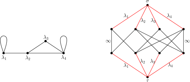
Figure 5: Left: A relation encoded as a graph, with intensities $\lambda_{1},\dots,\lambda_{4}$ for the four colours. Right: The corresponding network with edge capacities.

Consider now the maximal flow from $\sigma$ to $\tau$ which is consistent with the given edge capacities, and let $f_{ij}$ be the flow through the edge $(s_{i},t_{j})$. By the Max Flow – Min Cut Theorem, the total flow $\sum_{i,j}f_{ij}$ equals the minimal capacity of a cutset of edges separating $\sigma$ from $\tau$. Such a minimal cutset cannot contain any edge $(s_{i},t_{j})$, as these have infinite capacity. If a cutset contains the edges $\{(\sigma,s_{i})\ :\ i\not\in S\}$, then to be a cutset it must contain all edges $\{(t_{j},\tau)\ :\ j\in N(S)\}$. Such a cutset has capacity

$$\lambda(S^{c})+\lambda(N(S))=\|\lambda\|_{1}-\lambda(S)+\lambda(N(S)),$$

This is strictly less than $\|\lambda\|_{1}$ if and only if $\lambda(S)>\lambda(N(S))$, i.e. if $S$ is deficient. Since taking $S=\emptyset$ gives a cutset of capacity $\|\lambda\|_{1}$, the maximal flow is $\|\lambda\|_{1}$ if and only if there is no deficient set.

We now argue that a flow of $\|\lambda\|_{1}$ exists if and only if $\lambda\in\operatorname{cone}(V)$. Indeed, if $\lambda\in\operatorname{cone}(V)$, then we have $\lambda=\sum a_{ij}(e_{i}+e_{j})$ with some $a_{ij}=0$ when $i\not\sim j$. Take a flow of $a_{ij}$ on each of the edges $(s_{i},t_{j})$ and $(s_{j},t_{i})$, with the convention that if $i=j$ the flow on $(s_{i},t_{i})$ is $2a_{i}i$. Take a flow at maximal capacity $\lambda_{i}$ on the edges $(\sigma,s_{i})$ and $(t_{i},\tau)$. This flow has the required total flow (and conserves mass at all vertices). Conversely, if there is a flow $f$ of size $\|\lambda\|_{1}$, let $a_{ij}=\frac{1}{2}(f_{ij}+f_{ji})$ and observe that $\sum_{ij}a_{ij}(e_{i}+e_{j})=2\lambda$, and so $\lambda\in\operatorname{cone}(V)$.

Thus $\lambda$ is outside the cone if and only if there is some deficient set $S$. If every set is excessive then the same holds for any sufficiently small perturbation of $\lambda$, and so $\lambda\in\operatorname{cone}(V)^{\circ}$. If there is some critical set, then since $S\not=N(S)$ there is some $x\in S\setminus N(S)$. Increasing $\lambda_{x}$ by any amount makes the set deficient. Thus if there is a critical set but no deficient set, $\lambda\in\partial\operatorname{cone}(V)$. ∎

8 Open questions

Factor matchings in higher dimensions.

What is the optimal tail behavior of a multicolour matching that is a factor (i.e. a deterministic, translation equivariant function) of the Poisson processes? Theorem 2 gives some information in the case $d=1$. For $d\geq 2$, the condition $\mathcal{L}\neq\mathbb{Z}^{q}$ is no longer a clear obstacle. Do there exist matchings with the same tail behaviour as in Theorem 1 even if $\mathcal{L}\neq\mathbb{Z}^{q}$?

Stable matchings.

When the allowed families all have size two, a matching is called stable if there do not exist two points that are closer to each other than to their respective partners, but that could form a legal family. Stable matchings in the one-colour and two-colour cases are investigated in [6]. For general multicolour matching in pairs, when does a perfect stable matching exist? When a stable matching exists, what can be said about $X$? See [5] for some progress in certain cases. When families may have more than two elements, there are many possible non-equivalent extensions of the notion of stability, and the questions of existence and properties are also of interest.

Non-crossing matchings.

A matching into pairs is called non-crossing if the line segments joining the points of each pair are pairwise disjoint. For processes in $\mathbb{R}^{2}$, the question of existence of a non-intersecting invariant matching in two dimensions is open even for the case of two colours of equal intensities. See [3]. Again, there are several ways to generalize this notion to other family types. For instance, one can ask that there is some choice of line segments connecting the points of each family so that the sets of line segments do not intersect each other. Alternatively, one could ask that the convex hulls of the families are disjoint. In the latter sense the question is not trivial in higher dimensions $d$, provided $d$ is at most twice the maximum family size.

Minimal matchings.

Still in the setting of matching in pairs, a matching is called minimal if any other valid matching resulting by re-matching some finite subset of points has a larger total length. This notion too can be extended in different ways to matchings with families of other sizes. Under what conditions does a minimal matching exist? This is open even in the case of two colour matching.

Refined tail behavior.

The lower and upper bounds on the tail of $X$ are generally close, but a gap still exists. For example, in the critical two dimensional case we know that $\mathbb{E}^{*}X=\infty$ and that ther is a matching with $\mathbb{P}^{*}(X>r)\leq C/r$. Could there be a matching with $\mathbb{P}^{*}(X>r)<C/(r\log r)$? In the underconstrained case there are lower and upper bounds $e^{-Cr^{d}}\leq\mathbb{P}(X>r)\leq e^{-cr^{d}}$. Can these bounds be replaced by $\mathbb{P}^{*}(X>r)=e^{-ar^{d}+o(r^{d})}$ with the same constant $a$ for both sides?

1. Bar Ilan University, Ramat Gan, Israel
   gidi.amir@gmail.com

2. University of British Columbia, Vancouver, Canada
   angel@math.ubc.ca

3. Microsoft Research, Redmond, USA
   holroyd@microsoft.com

References

- [1] Itai Benjamini, Russell Lyons, Yuval Peres, and Oded Schramm. Uniform spanning forests. Ann. Probab., 29(1):1–65, 2001.
- [2] Itai Benjamini and Oded Schramm. Percolation in the hyperbolic plane [mr1815220]. J. Amer. Math. Soc., 14(2):487–507 (electronic), 2001.
- [3] Alexander E. Holroyd. Geometric properties of Poisson matchings. Probability Theory and Related Fields, 150(3):511–527, 2011.
- [4] Alexander E. Holroyd and Tom M. Liggett. How to find an extra head: optimal random shifts of Bernoulli and Poisson random fields. Ann. Probab., 29(4):1405-1425, 2001.
- [5] Alexander E. Holroyd, James B. Martin, and Yuval Peres. Asymmetric stable matchings in high dimensions. In preparation.
- [6] Alexander E. Holroyd, Robin Pemantle, Yuval Peres, and Oded Schramm. Poisson matching. Ann. Inst. Henri Poincare Probab. Stat., 2009.
- [7] O. Kallenberg. Foundations of Modern Probability. Springer, 2nd edition edition, 2002.
- [8] Russell Lyons and Yuval Peres. Probability on trees and networks. book in preparation, 2015.
- [9] R. T. Rockafellar. Convex analysis. Number 28 in Princeton Mathematical Series. Princeton University Press, 1970.
- [10] Edward R. Scheinerman and Daniel H. Ullman. Fractional Graph Theory. Wiley and Sons, 2008.
- [11] Adam Timar. Invariant matchings of exponential tail on coin flips in . arXiv:0909.1090, 2009.
- [12] William T. Tutte. The factorization of linear graphs. J. London Math. Soc., 22:107–111, 1947.
-
Gideon Amir
Bar Ilan University, Ramat Gan, Israel