X-ray Image Separation via Coupled Dictionary Learning

Abstract

In support of art investigation, we propose a new source separation method that unmixes a single X-ray scan acquired from double-sided paintings. Unlike prior source separation methods, which are based on statistical or structural incoherence of the sources, we use visual images taken from the front- and back-side of the panel to drive the separation process. The coupling of the two imaging modalities is achieved via a new multi-scale dictionary learning method. Experimental results demonstrate that our method succeeds in the discrimination of the sources, while state-of-the-art methods fail to do so.

Index Terms— Image separation, side information, dictionary learning, image decomposition, multi-modal imaging.

1 Introduction

The analysis and enhancement of high-resolution digital acquisitions of paintings is becoming a popular field of research [1, 2]. Prior work includes the removal of canvas artifacts in high-resolution photographs [3], the removal of cradling in X-ray images of paintings on panel [4], as well as the detection and digital removal of cracks  [5].

In this work, we propose a novel framework to separate X-ray images taken from double-sided paintings. A famous piece of art that contains panels painted on both sides is the Ghent Altarpiece (1432) created by Jan and Hubert van Eyck. In preparation of its restoration, the masterpiece was digitized by means of various modalities: visual photography, infrared photography and reflectography, and X-radiography [6]. The latter is a powerful tool for art investigation, as it reveals information about the structural condition of the painting. However, X-ray scans of double-sided paintings are very cluttered, thus making their reading by art experts difficult. The reason is that these images contain information from both sides of the painting as well as its support (wood structure or canvas).

Prior work on umixing signals focuses mostly on the blind source separation (BSS) problem, where the task is to retrieve the different signal sources from one or more linear mixtures. Independent component analysis (ICA) [7]—where the sources are assumed to be statistically independent—and nonnegative matrix factorization—where the sources are considered or transformed into a nonnegative representation [8]—are representative methods to solve the BSS problem. Alternative solutions adhere to a Bayesian formulation, via, for example, Markov random fields [9]. Sparsity is another source prior, heavily exploited in BSS problems [10, 11], with morphological component analysis (MCA) being a state-of-the-art method. The assumption in MCA is that each source has a different morphology; namely, it has a sparse representation over a set of bases, alias, dictionaries, while being non-sparse over other dictionaries. The dictionaries can be pre-defined, for instance, the wavelet or the discrete cosine transform (DCT), or learned from a set of training signals. Seminal dictionary learning works include the method of optimal directions (MOD) [12] and the K-SVD algorithm [13], both utilizing the orthogonal matching pursuit (OMP) [14] method to perform sparse signal decomposition. Recently, MCA has been combined with K-SVD, thus enabling dictionaries to be learned while separating [15].

The assumptions in previous source separation methods are not fitting our problem as both sources have similar morphological and statistical traits. In this work, we propose a novel method to perform separation of X-ray images of paintings by using images of another modality as side information. Our approach consists of two steps: 1) learning multi-scale dictionaries from photographs and X-rays of single-sided panels (in which the X-rays are not mixed), and 2) separating the given mixed X-ray from a double-sided panel, using those dictionaries and the photographs from each side. Previous work has used coupled dictionary learning to address problems in audio-visual analysis [16], super-resolution [17], photo-sketch synthesis[18], and human pose estimation [19]. Besides the application domain, our method differs from prior work in the way we model the correlation between the sources. Experimental evidence proves that our method is superior compared to the state-of-the-art MCA technique, configured either with fixed or trained dictionaries.

2 Image Separation with Side Information

We start by describing MCA, as the state-of-the-art sparsity based source separation method, and afterwards we introduce the proposed method which, unlike the former, makes use of side information. First, let us denote by $x_{1}\in\mathbb{R}^{n\times 1}$ and $x_{2}\in\mathbb{R}^{n\times 1}$ two vectorized X-ray image patches that we wish to separate from a given X-ray scan patch $m=x_{1}+x_{2}$.
Morphological Component Analysis. Assume that each $x_{i}$ admits a sparse decomposition in a different overcomplete dictionary $\Lambda_{i}\in\mathbb{R}^{n\times d_{i}}$, $(n\ll\ d_{i})$; namely, each component can be expressed as $x_{i}=\Lambda_{i}z_{i}$, where $z_{i}\in\mathbb{R}^{d_{i}\times 1}$ is a sparse vector comprising a few non-zero coefficients: $\|z_{i}\|_{0}=s_{i}\ll d_{i}$, with $\|\cdot\|_{0}$ denoting the $\ell_{0}$ pseudo-norm. MCA [10, 11] decomposes the mixture by approximately solving the following optimization problem:

$$\begin{array}[]{ll}\underset{z_{1},z_{2}}{\text{minimize}}&\|z_{1}\|_{0}+\|z_{2}\|_{0}\\ \text{subject to}&m=\Lambda_{1}z_{1}+\Lambda_{2}z_{2}\\ \end{array}$$ (3)

A typical approximation consists of replacing the $\ell_{0}$ pseudo-norm with the $\ell_{1}$-norm.
Source Separation with Side Information. The use of side information has proven beneficial in various inverse problems [20, 21, 22]. Adhering to this logic, we show how side information can be helpful in separating mixtures, where the sources have similar characteristics. In our particular problem, we consider side information signals $y_{1}$ and $y_{2}$ formed by the co-located visual image patches of the front and the back of the painting. Both the X-ray and side information signals admit a sparse decomposition in given dictionaries, namely,

$$y_{1} =\Psi^{c}z_{1c}$$

$$y_{2} =\Psi^{c}z_{2c}\ ,$$ (4)

and

$$x^{ray}_{1} =\Phi^{c}z_{1c}+\Phi v$$

$$x^{ray}_{2} =\Phi^{c}z_{2c}+\Phi v_{,}$$ (5)

where $z_{ic}\in\mathbb{R}^{\gamma\times 1}$, with $\|z_{ic}\|_{0}=s_{z}\ll\gamma$, denotes the sparse component that is common to the visual and X-ray images with respect to dictionaries $\Psi^{c},\Phi^{c}\in\mathbb{R}^{n\times{\gamma}}$. Moreover, $v\in\mathbb{R}^{d\times{1}}$, with $\|v\|_{0}=s_{v}\ll d$, denotes the sparse innovation component of the X-ray image, obtained with respect to dictionary $\Phi\in\mathbb{R}^{n\times{d}}$. The common components express the structure underlying both the X-ray and natural images, while the innovation component captures X-ray specific parts of the signal (e.g., traces of the wooden panel). The separation problem is now formulated as the following problem:

$$\begin{array}[]{ll}\underset{z_{c1},z_{c2},v}{\text{minimize}}&\|z_{c1}\|_{0}+\|z_{c2}\|_{0}+\|v\|_{0}\\ \text{subject to}&m=\Phi^{c}z_{1c}+\Phi^{c}z_{2c}+2\Phi v\\ &y_{1}=\Psi^{c}z_{1c}\\ &y_{2}=\Psi^{c}z_{2c}\end{array}$$ (10)

The relaxed version of Problem (10) boils down to Basis Pursuit, which is solved by convex optimization tools, e.g., [23].

Algorithm 1 modified Orthogonal Matching Pursuit

1:

2:

3:Initialize residual: $r_{0}=b$.

4:Total sparsity of vector $w$: $s_{w}=s_{z}+s_{v}$.

5:Counters for the sparsity of $z$ and $v$: $\ell_{z}=0$, $\ell_{v}=0$.

6:Set of non-zero elements of $w$: $\Omega=\emptyset$.

7:

8:

9:for $i=1,2,\dots,s_{w}$ do

10:    Sort the indices $\zeta=\{1,2,\dots,\gamma+d\}$, corresponding to the $\theta_{\zeta}$ columns of $\Theta$, such that $|\langle r_{i-1},\theta_{\zeta}\rangle|$ are in descending order. Put the ordered indices in the vector $q_{i}$.

11:    Set $\mathcal{G}=\emptyset$ and auxiliary iterator $\texttt{it}=0$.

12:    while $\mathcal{G}=\emptyset$ do

13:         it=it+1.

14:         Find index that corresponds to value of it: $\kappa=q_{i}[\texttt{it}]$.

15:         if $\kappa\in\mathcal{I}$ AND $\ell_{z}<s_{z}$ then

16:             Set $\mathcal{G}=\kappa$ and increase: $\ell_{z}=\ell_{z}+1$.

17:         else

18:             if $\kappa\in\mathcal{J}$ AND $\ell_{v}<s_{v}$ then

19:                 Set $\mathcal{G}=\kappa$ and increase : $\ell_{v}=\ell_{v}+1$.

20:             end if

21:         end if

22:    end while

23:    Update the set of non-zero elements of $w$, i.e., $\Omega_{i}=\Omega_{i-1}\cup\{\kappa\}$, and the matrix of chosen atoms: $\Theta_{i}=[\Theta_{i-1}\quad\theta_{\kappa}]$.

24:    Solve: $w_{i}=\arg\min_{w}\|b-\Theta_{i}w\|_{2}$.

25:    Calculate the new residual: $r_{i}=b-\Theta_{i}w_{i}$.

26:end for

3 Coupled Dictionary Learning Algorithm

We train coupled dictionaries, $\Psi^{c}$, $\Phi^{c}$, $\Phi$, by using image patches sampled from registered visual and X-ray images of single-sided panels, which do not suffer from superposition phenomena. Let $Y,X\in\mathbb{R}^{n\times t}$ represent a set of $t$ co-located vectorized visual and X-ray patches, each containing $\sqrt{n}\times\sqrt{n}$ pixels. We assume that the columns of $X$ and $Y$ can be decomposed as in (2), and we collect their common components into the columns of the matrix $Z\in\mathbb{R}^{\gamma\times t}$ and their innovation components into the columns of $V\in\mathbb{R}^{d\times{t}}$. We formulate the coupled dictionary learning problem as

$$\begin{array}[t]{cl}\underset{\begin{subarray}{\hfil\lx@intercol{\\ }}\Psi^{c},Z\\ \Phi^{c},\Phi,V\end{subarray}}{\text{minimize}}&\frac{1}{2}\big{\|}Y-\Psi^{c}Z\big{\|}_{F}^{2}+\frac{1}{2}\big{\|}X-\Phi^{c}Z-\Phi V\big{\|}_{F}^{2},\\ \text{subject to}&\big{\|}z_{\tau}\big{\|}_{0}\leq s_{z},\vspace{0.2cm}\par\\ &\big{\|}v_{\tau}\big{\|}_{0}\leq s_{v},\quad\forall\tau=1,2,\dots t,\end{array}$$ (11)

where $z_{\tau}$, $v_{\tau}$ are sparse vector-columns of matrix $Z$ and $V$, $\tau$ runs over the columns of $Z$ and $V$, and $s_{z}$, $s_{v}$ are thresholds on the sparsity level. Given initial estimates for the dictionaries, Problem (11) is solved by iterating between a sparse-coding step, where the dictionaries are fixed, and a dictionary update step, in which the coefficients are fixed, as in [13, 12].

Given fixed dictionaries, the sparse coding problem decomposes into $t$ problems that can be solved in parallel:

$$(z_{\tau}^{k+1},v_{\tau}^{k+1})=\begin{array}[t]{cl}\underset{\quad\;z_{\tau},v_{\tau}}{\text{arg}\;\text{min}}&\frac{1}{2}\Bigg{\|}\begin{bmatrix}y_{\tau}\\ x_{\tau}\end{bmatrix}\par-\begin{bmatrix}{\Psi^{c}}^{k}&0\\ {\Phi^{c}}^{k}&\Phi^{k}\end{bmatrix}\begin{bmatrix}z_{\tau}\\ v_{\tau}\end{bmatrix}\vspace{0.2cm}\Bigg{\|}_{F}^{2},\\ \text{subject to}&\big{\|}z_{\tau}\big{\|}_{0}\leq s_{z},\vspace{0.2cm}\\ &\big{\|}v_{\tau}\big{\|}_{0}\leq s_{v},\quad\forall\tau=1,2,\dots t,\end{array}$$ (12)

where we used $x_{\tau}$, $y_{\tau}$, $z_{\tau}$, and $v_{\tau}$ to represent column $\tau$ of $X$, $Y$, $Z$, and $V$, respectively, and $k$ counts the iterations. To address each of the $t$ sub-problems in (12), we propose a greedy algorithm that constitutes a modification of the OMP method [see Algorithm 1]. Our method adapts OMP [14] to solve:

$$\begin{array}[]{cc}\underset{w}{\text{minimize}}&\|b-\Theta w\|_{2}^{2}\\ \text{subject to}&\|(w(\mathcal{I})\|_{0}\leq s_{z},\\ &\|w(\mathcal{J})\|_{0}\leq s_{v},\end{array}$$ (16)

where $w(\mathcal{I})$ [resp., $w(\mathcal{J})$] denotes the components of vector $w\in\mathbb{R}^{(\gamma+d)\times 1}$ indexed by the index set $\mathcal{I}$ (resp., $\mathcal{J}$), with $\mathcal{I}\cup\mathcal{J}=\{1,2,\dots,\gamma+d\}$, $\mathcal{I}\cap\mathcal{J}=\{\O\}$. Each sub-problem in (12) translates to (16) by replacing: $b=\begin{bmatrix}y_{\tau}\\ x_{\tau}\end{bmatrix}$, $\Theta=\begin{bmatrix}{\Psi^{c}}^{k}&0\\ {\Phi^{c}}^{k}&\Phi^{k}\end{bmatrix}$, and $w=\begin{bmatrix}z_{\tau}\\ v_{\tau}\end{bmatrix}$.

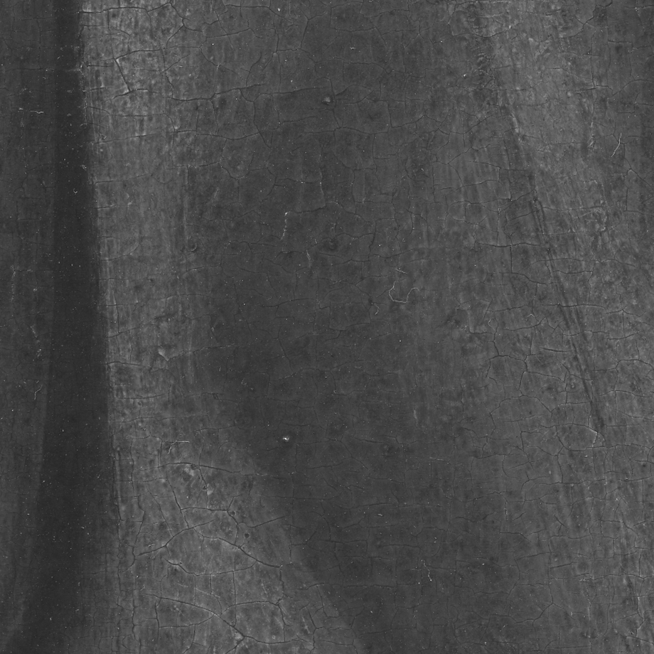
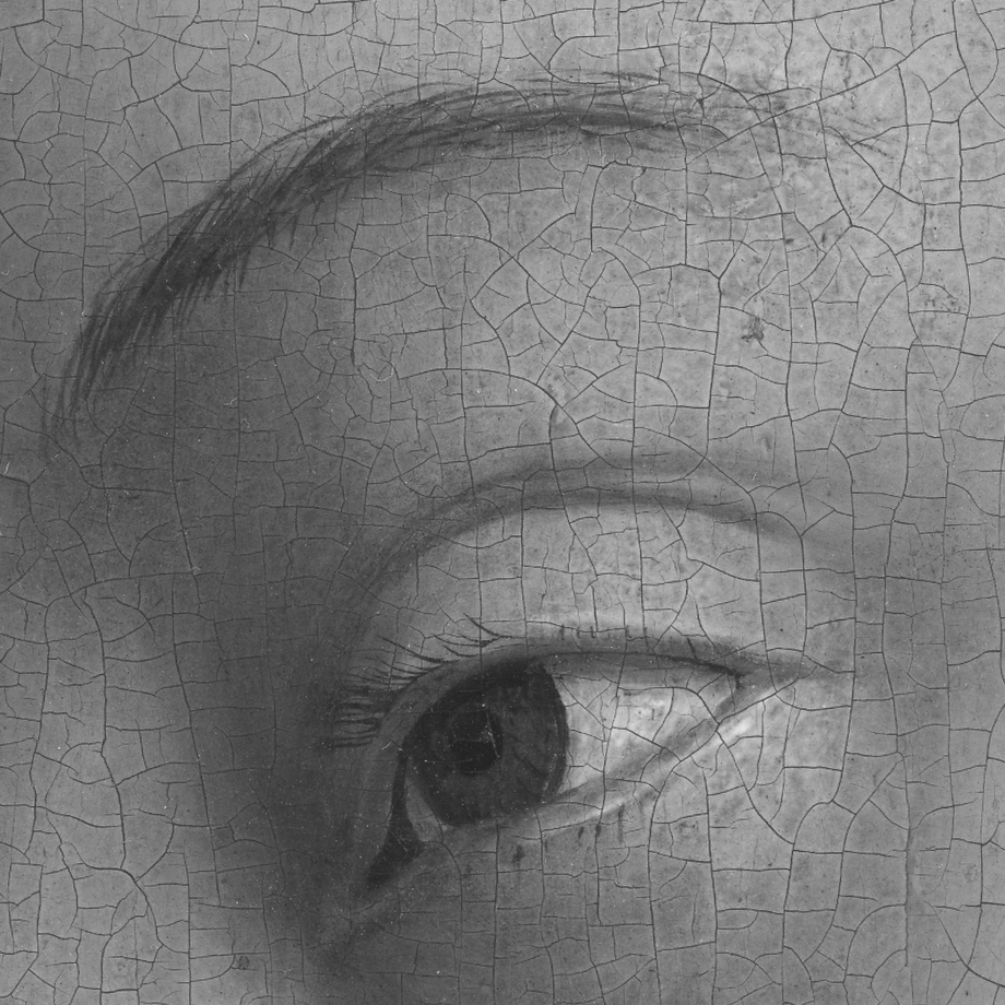
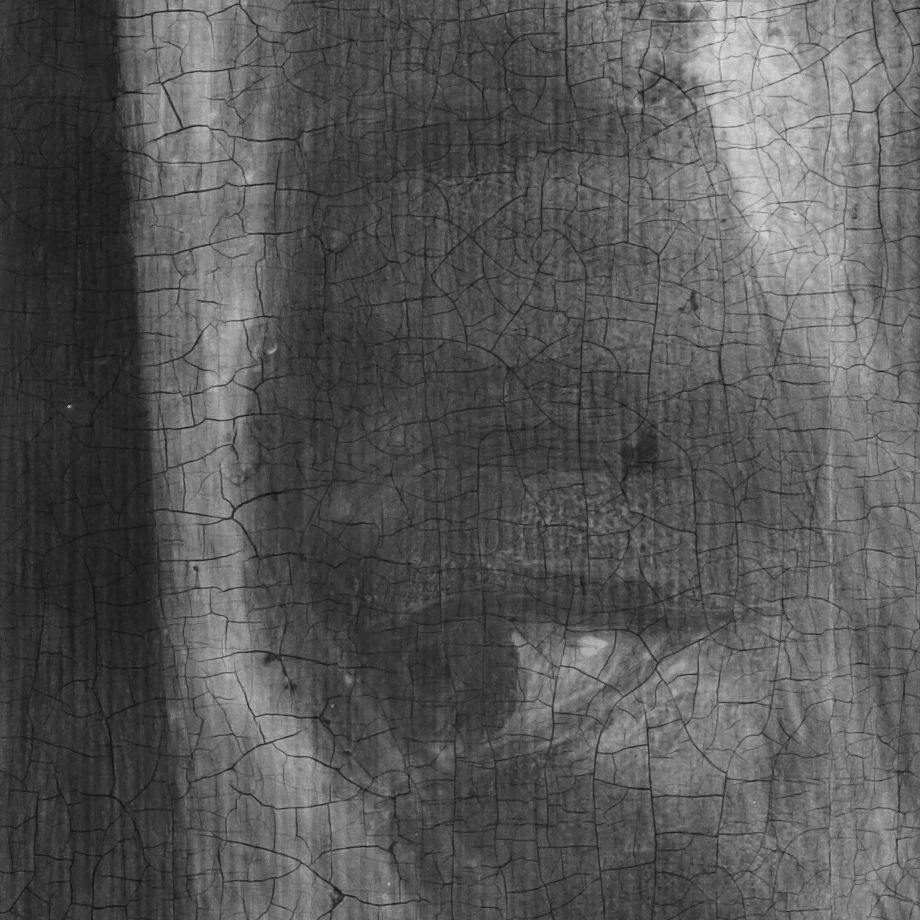
Fig. 1: Image set cropped from a double-sided panel of the altarpiece, on which we assess the proposed method; (a) photograph of side 1, (b) photograph of side 2; (c) corresponding X-ray image. The resolution is $1024\times{1024}$ pixels.

Given fixed sparse coefficients, the dictionary update problem decouples into two (independent) problems, that is,

$${\Psi^{c}}^{k+1}=\arg\min_{\Psi^{c}}\frac{1}{2}\Big{\|}Y-\Psi^{c}\cdot Z^{k+1}\Big{\|}_{F}^{2}$$

and

$$\overline{\Phi}^{k+1}=\arg\min_{\overline{\Phi}}\frac{1}{2}\Big{\|}X-\overline{\Phi}\cdot\overline{V}^{k+1}\Big{\|}_{F}^{2},$$

where $\overline{\Phi}=\begin{bmatrix}\Phi^{c}&\Phi\end{bmatrix}$ and $\overline{V}^{k+1}=\begin{bmatrix}Z^{k+1}\\ V^{k+1}\end{bmatrix}$. Each of these problems has a closed-form solution.

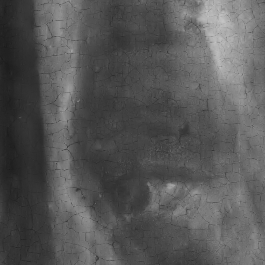
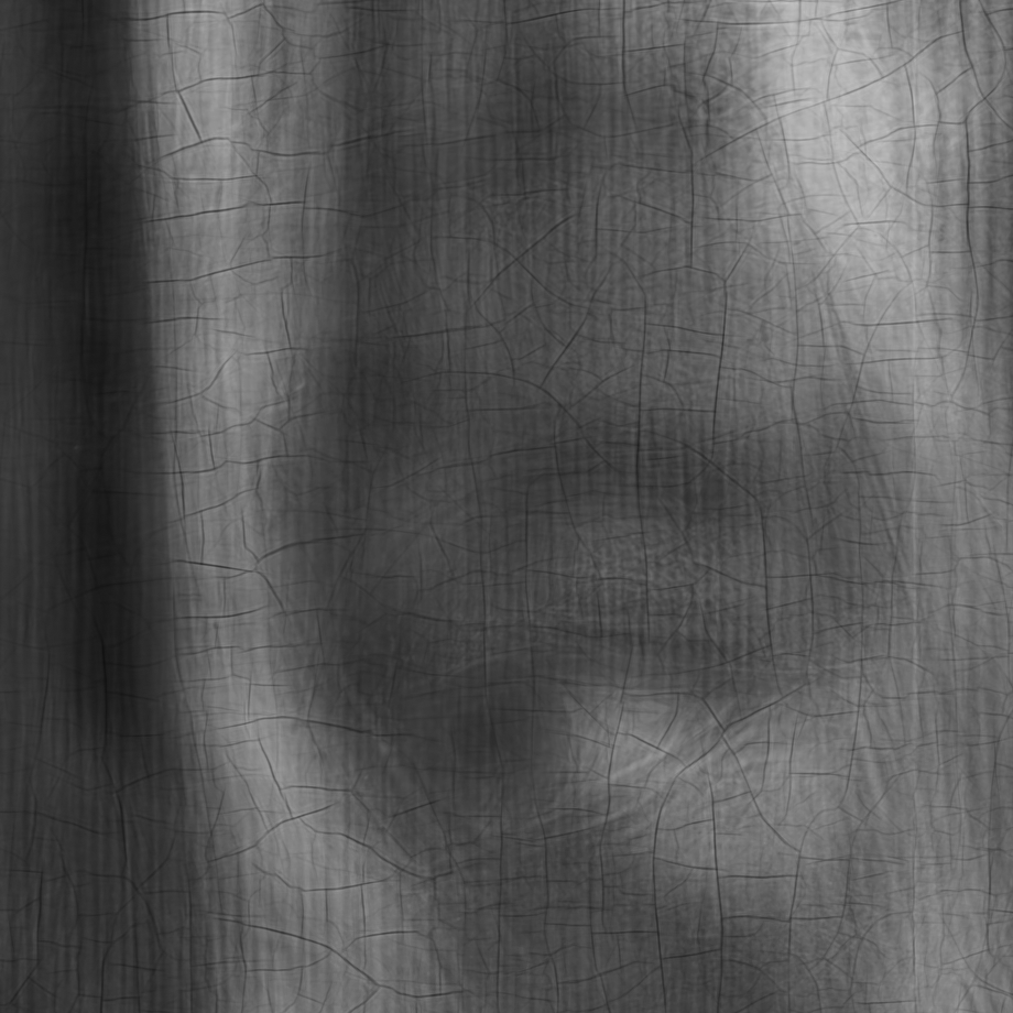
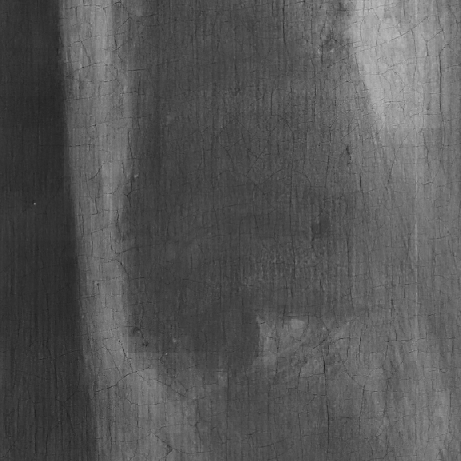
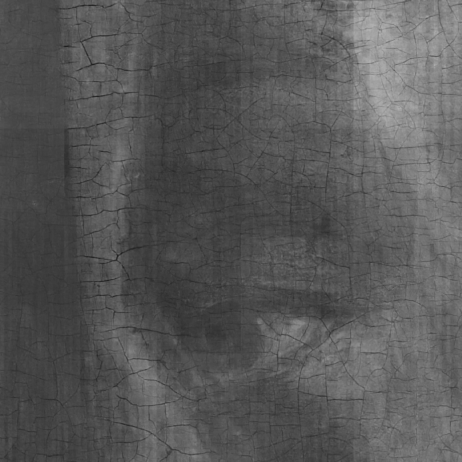
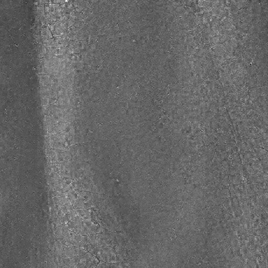
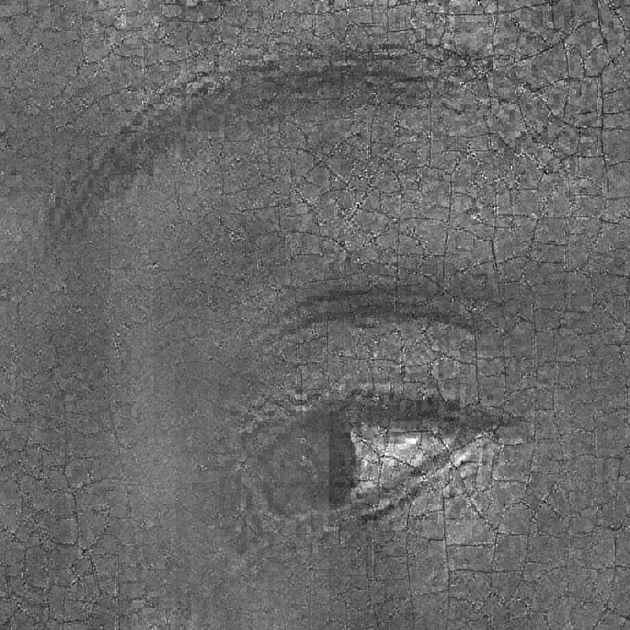
Fig. 2: Visual evaluation of the proposed multi-scale method in the separation of the X-ray in Fig. 1(c); (left) separated side 1, (right) separated side 2. The competing methods are: (1st row) MCA with fixed dictionaries [4], (2nd row) multi-scale MCA with K-SVD, (3rd row) Proposed.

4 X-ray Image Separation Method

Because of complexity, dictionaries are learned for small image patches, usually with dimensions of $8\times 8$ pixels; namely, we adhere to a local sparsity prior. However, due to the high-resolution of the images, patches of that size cannot fully capture large structures. Hence, we propose a multi-scale image separation approach that is based on a pyramid decomposition of the images. Our multi-scale strategy is as follows: The images at scale $l=\{1,2,\dots,L\}$—where we use the notation $M_{l},Y_{1,l},Y_{2,l}$, to refer to the mixed X-ray and the two visuals, respectively—are divided into overlapping patches $m_{l}^{\boldsymbol{u}_{l}},y_{1,l}^{\boldsymbol{u}_{l}},\>\text{and}\>y_{2,l}^{\boldsymbol{u}_{l}}$, each of size $\sqrt{n_{l}}\times\sqrt{n_{l}}$ pixels. Each patch has top-left coordinates

$$\boldsymbol{u}_{l}=(\epsilon_{l}\cdot u_{1,l},\epsilon_{l}\cdot u_{2,l}),\>0\leq u_{1,l}<\left\lfloor\frac{H_{l}}{\epsilon_{l}}\right\rfloor,\>0\leq u_{2,l}<\left\lfloor\frac{W_{l}}{\epsilon_{l}}\right\rfloor,$$

where $\epsilon_{l}\in\mathbb{Z}_{+},\>\sqrt{n_{l}}\leq\epsilon_{l}<\sqrt{n_{l}}$ is the overlap step-size, and $H_{l},W_{l}$ are the height and width of the image decomposition at scale $l$. The DC value is extracted from each patch, thereby constructing the high frequency band of the image at scale $l$. The aggregated DC values comprise the low-pass component of the image, the resolution of which is $\left\lfloor\frac{H_{l}}{\epsilon_{l}}\right\rfloor\times\left\lfloor\frac{W_{l}}{\epsilon_{l}}\right\rfloor$ pixels. The low-pass component is then decomposed further at the subsequent scale ($l+1$). The texture of the mixed X-ray image at scale $l$ is separated patch-per-patch by solving Problem (10). The texture of each separated patch is then reconstructed as $x_{1,l}^{\boldsymbol{u}_{l}}=\Phi^{c}_{l}z_{1c,l}^{\boldsymbol{u}_{l}}$ and $x_{2,l}^{\boldsymbol{u}_{l}}=\Phi_{l}^{c}z_{2c,l}^{\boldsymbol{u}_{l}}$. Namely, we omit the innovation component $v$ [see (2)] during reconstruction, as this is common to the two X-rays. The separated X-ray images are finally reconstructed by following the reverse operation: Descending the pyramid, the separated component at the coarser level is up-sampled and added to the separated component of the finer scales.

As a final note, the dictionary learning process is applied per scale, yielding a triple of coupled dictionaries $(\Psi^{c}_{l},\Phi^{c}_{l},\Phi_{l})$ per scale $l$. Due to lack of training data in the coarser scales, dictionaries are typically learned on the finer scales and then re-used in the coarsest scale.

5 Experiments

We assess our method on different crops, with dimensions of $1024\times 1024$, taken from the digital acquisitions [6] of one double-sided panel of the Ghent Altarpiece (1432). An example X-ray image we aim to separate and the two corresponding visual images from each side of the panel are depicted in Fig. 1. We apply the multi-scale framework, where we use $L=3$ scales with parameters $\sqrt{n_{l}}=8$, $\epsilon_{1}=4$, $\epsilon_{2}=4$ and $\epsilon_{3}=7$. Dictionary triplets $(\Psi^{c}_{\ell},\Phi^{c}_{\ell},\Phi_{\ell})$, each with dimension of $64\times{256}$, are trained for the first two layers and the dictionaries of the second layer are extrapolated to the third. We use $t=46000$ patches from digital acquisitions of the single-sided panels of the altarpiece and set $s_{z}=10$ and $s_{v}=8$.

To demonstrate the benefit of using side information, we compare our method against two configurations of MCA [10, 11]. In the first one we use the discrete wavelet and curvelet transforms on blocks of $512\times 512$ pixels [4]; the low-frequency content is divided between the two components. In the second configuration we use K-SVD to train two dictionaries: one on X-ray images depicting cloth and the other on images depicting faces—content also found in the X-ray mixtures. The K-SVD method is extended with our multi-scale strategy and the same parameters are used. As no ground truth data is available, we first resort to visual comparisons. The results, depicted in Fig. 2, clearly show that MCA with fixed dictionaries can only separate based on morphological properties; for example, the wood grain of the panel is captured entirely by curvelets and not by the wavelets. It is, however, unfitted to separate painted content. MCA with K-SVD dictionaries is also unable to separate the X-ray content as the dictionaries are not sufficiently discriminative. The results using our method show the benefit of incorporating side information in the separation problem. Towards a more objective comparison, we measure the structural similarity (SSIM) [24] index between the two separated components, where low SSIM values would indicate less similarity; hence good separation. The results on two additional X-ray scans from the same painting, reported in Table 1, confirm the better separation performance of our method, as advocated by the lowest SSIM values.

Table 1: Similarity scores (obtained with the SSIM [24] metric) between the separated components.

	MCA fixed	MCA trained	Proposed
X-ray mixture 1	0.9249	0.7385	0.1681
X-ray mixture 2	0.9603	0.8341	0.6034

6 Conclusion

We have proposed a novel sparsity-based regularization method for source separation guided by side information. Our method is based on a new multi-scale algorithm that learns dictionaries coupling multi-modal data. We apply the proposed method to separate X-ray images of paintings with content on both sides of their panel, where photographs of each side are used as side information. Experiments with real data from digital acquisitions of the Ghent Altarpiece (1432), prove the superiority of our method compared to the state-of-the-art MCA technique [10, 11, 15].

References

- [1] L. van der Maaten and R.G. Erdmann, “Automatic thread-level canvas analysis: A machine-learning approach to analyzing the canvas of paintings,” IEEE Signal Process. Mag., vol. 32, no. 4, pp. 38–45, July 2015.
- [2] N. van Noord, E. Hendriks, and E. Postma, “Toward discovery of the artist’s style: Learning to recognize artists by their artworks,” IEEE Signal Process. Mag., vol. 32, no. 4, pp. 46–54, July 2015.
- [3] B. Cornelis, A. Dooms, J. Cornelis, and P. Schelkens, “Digital canvas removal in paintings,” Signal Process., vol. 92, no. 4, pp. 1166–1171, 2012.
- [4] R. Yin, D. Dunson, B. Cornelis, B. Brown, N. Ocon, and I. Daubechies, “Digital cradle removal in X-ray images of art paintings,” in IEEE ICIP, 2014, pp. 4299–4303.
- [5] B. Cornelis, T. Ružić, E. Gezels, A. Dooms, A. Pižurica, L. Platiša, J. Cornelis, M. Martens, M. De Mey, and I. Daubechies, “Crack detection and inpainting for virtual restoration of paintings: The case of the Ghent Altarpiece,” Signal Process., 2012.
- [6] A. Pizurica, L. Platisa, T. Ruzic, B. Cornelis, A. Dooms, M. Martens, H. Dubois, B. Devolder, M. De Mey, and I. Daubechies, “Digital image processing of the Ghent Altarpiece: Supporting the painting’s study and conservation treatment,” IEEE Signal Process. Mag., vol. 32, no. 4, pp. 112–122, 2015.
- [7] A. Hyvärinen, J. Karhunen, and E. Oja, Independent component analysis, vol. 46, John Wiley & Sons, 2004.
- [8] P. Smaragdis, C. Févotte, G. Mysore, N. Mohammadiha, and M. Hoffman, “Static and dynamic source separation using nonnegative factorizations: A unified view,” IEEE Signal Process. Mag., vol. 31, no. 3, pp. 66–75, 2014.
- [9] K. Kayabol, E. Kuruoğlu, and B. Sankur, “Bayesian separation of images modeled with MRFs using MCMC,” IEEE Trans. Image Process., vol. 18, no. 5, pp. 982–994, 2009.
- [10] J. Bobin, J.-L. Starck, J. Fadili, and Y. Moudden, “Sparsity and morphological diversity in blind source separation,” IEEE Trans. Image Process., vol. 16, no. 11, pp. 2662–2674, 2007.
- [11] M. Zibulevsky and B. Pearlmutter, “Blind source separation by sparse decomposition in a signal dictionary,” Neural computation, vol. 13, no. 4, pp. 863–882, 2001.
- [12] K. Engan, S. O. Aase, and J. Hakon-Husoy, “Method of optimal directions for frame design,” in IEEE ICASSP, 1999, pp. 2443–2446.
- [13] M. Aharon, M. Elad, and A. Bruckstein, “K-SVD: An algorithm for designing overcomplete dictionaries for sparse representation,” IEEE Trans. Signal Process., vol. 54, no. 11, pp. 4311–4322, Nov. 2006.
- [14] J. A. Tropp and A. C. Gilbert, “Signal recovery from random measurements via orthogonal matching pursuit,” IEEE Trans. Inf. Theory, vol. 53, no. 12, pp. 4655–4666, 2007.
- [15] V. Abolghasemi, S. Ferdowsi, and S. Sanei, “Blind separation of image sources via adaptive dictionary learning,” IEEE Trans. Image Process., vol. 21, no. 6, pp. 2921–2930, 2012.
- [16] G. Monaci, P. Jost, P. Vandergheynst, B. Mailhe, S. Lesage, and R. Gribonval, “Learning multimodal dictionaries,” IEEE Trans. Image Process., vol. 16, no. 9, pp. 2272–2283, 2007.
- [17] J. Yang, Z. Wang, Z. Lin, S. Cohen, and T. Huang, “Coupled dictionary training for image super-resolution,” IEEE Trans. Image Process., vol. 21, no. 8, pp. 3467–3478, 2012.
- [18] S. Wang, L. Zhang, Y. Liang, and Q. Pan, “Semi-coupled dictionary learning with applications to image super-resolution and photo-sketch synthesis,” in IEEE CVPR, 2012, pp. 2216–2223.
- [19] Y. Jia, M. Salzmann, and T. Darrell, “Factorized latent spaces with structured sparsity,” in Advances in Neural Information Processing Systems, 2010, pp. 982–990.
- [20] N. Vaswani and W. Lu, “Modified-cs: Modifying compressive sensing for problems with partially known support,” IEEE Trans. Signal Process., vol. 58, no. 9, pp. 4595–4607, 2010.
- [21] J. F. C. Mota, N. Deligiannis, and M. R. D. Rodrigues, “Compressed sensing with prior information: Optimal strategies, geometry, and bounds,” arXiv preprint arXiv:1408.5250, 2014.
- [22] J. F. C. Mota, N. Deligiannis, and M. R. D. Rodrigues, “Compressed sensing with side information: Geometrical interpretation and performance bounds,” in IEEE GlobalSIP, 2014, pp. 512–516.
- [23] E. van den Berg and M. P. Friedlander, “Probing the Pareto frontier for basis pursuit solutions,” SIAM Journal on Scientific Computing, vol. 31, no. 2, pp. 890–912, 2008.
- [24] Z. Wang, A. C. Bovik, H. R. Sheikh, and E. P. Simoncelli, “Image quality assessment: from error visibility to structural similarity,” IEEE Trans. Image Process., vol. 13, no. 4, pp. 600–612, 2004.