Swapout: Learning an ensemble of deep architectures
Abstract
We describe Swapout, a new stochastic training method, that outperforms ResNets of identical network structure yielding impressive results on CIFAR-10 and CIFAR-100. Swapout samples from a rich set of architectures including dropout [17], stochastic depth [6] and residual architectures [4, 5] as special cases. When viewed as a regularization method swapout not only inhibits co-adaptation of units in a layer, similar to dropout, but also across network layers. We conjecture that swapout achieves strong regularization by implicitly tying the parameters across layers. When viewed as an ensemble training method, it samples a much richer set of architectures than existing methods such as dropout or stochastic depth. We propose a parameterization that reveals connections to exiting architectures and suggests a much richer set of architectures to be explored. We show that our formulation suggests an efficient training method and validate our conclusions on CIFAR-10 and CIFAR-100 matching state of the art accuracy. Remarkably, our 32 layer wider model performs similar to a 1001 layer ResNet model.
1 Introduction
This paper describes swapout, a stochastic training method for general deep networks. Swapout is a generalization of dropout [17] and stochastic depth [6] methods. Dropout zeros the output of individual units at random during training, while stochastic depth skips entire layers at random during training. In comparison, the most general swapout network produces the value of each output unit independently by reporting the sum of a randomly selected subset of current and all previous layer outputs for that unit. As a result, while some units in a layer may act like normal feedforward units, others may produce skip connections and yet others may produce a sum of several earlier outputs. In effect, our method averages over a very large set of architectures that includes all architectures used by dropout and all used by stochastic depth.
Our experimental work focuses on a version of swapout which is a natural generalization of the residual network [4, 5]. We show that this results in improvements in accuracy over residual networks with the same number of layers.
Improvements in accuracy are often sought by increasing the depth, leading to serious practical difficulties. The number of parameters rises sharply, although recent works such as [16, 19] have addressed this by reducing the filter size [16, 19]. Another issue resulting from increased depth is the difficulty of training longer chains of dependent variables. Such difficulties have been addressed by architectural innovations that introduce shorter paths from input to loss either directly [19, 18, 4] or with additional losses applied to intermediate layers [19, 10]. At the time of writing, the deepest networks that have been successfully trained are residual networks (1001 layers [5]). We show that increasing the depth of our swapout networks increases their accuracy.
There is compelling experimental evidence that these very large depths are helpful, though this may be because architectural innovations introduced to make networks trainable reduce the capacity of the layers. The theoretical evidence that a depth of 1000 is required for practical problems is thin. Bengio and Dellaleau argue that circuit efficiency constraints suggest increasing depth is important, because there are functions that require exponentially large shallow networks to compute [1]. Less experimental interest has been displayed in the width of the networks (the number of filters in a convolutional layer). We show that increasing the width of our swapout networks leads to significant improvements in their accuracy; an appropriately wide swapout network is competitive with a deep residual network that is 1.5 orders of magnitude deeper and has more parameters.
Contributions: Swapout is a novel stochastic training scheme that can sample from a rich set of architectures including dropout, stochastic depth and residual architectures as special cases. Swapout improves the performance of the residual networks for a model of the same depth. Wider but much shallower swapout networks are competitive with very deep residual networks.
2 Related Work
Convolutional neural networks have a long history (see the introduction of [9]). They are now intensively studied as a result of recent successes (e.g. [8]). Increasing the number of layers in a network improves performance [16, 19] if the network can be trained. A variety of significant architectural innovations improve trainability, including: the ReLU [12, 2]; batch normalization [7]; and allowing signals to skip layers.
Our method exploits this skipping process. Highway networks use gated skip connections to allow information and gradients to pass unimpeded across several layers [18]. Residual networks use identity skip connections to further improve training [4]; extremely deep residual networks can be trained, and perform well [5]. In contrast to these architectures, our method skips at the unit level (below), and does so randomly.
Our method employs randomness at training time. For a review of the history of random methods, see the introduction of [14], which shows that entirely randomly chosen features can produce an SVM that generalizes well. Randomly dropping out unit values (dropout [17]) discourages co- adaptation between units. Randomly skipping layers (stochastic depth) [6] during training reliably leads to improvements at test time, likely because doing so regularizes the network. The precise details of the regularization remain uncertain, but it appears that stochastic depth represents a form of tying between layers; when a layer is dropped, other layers are encouraged to be able to replace it. Each method can be seen as training a network that averages over a family of architectures during inference. Dropout averages over architectures with “missing” units and stochastic depth averages over architectures with “missing” layers. Other successful recent randomized methods include dropconnect [20] which generalizes dropout by dropping individual connections instead of units (so dropping several connections together), and stochastic pooling [21] (which regularizes by replacing the deterministic pooling by randomized pooling). In contrast, our method skips layers randomly at a unit level enjoying the benefits of each method.
Recent results show that (a) stochastic gradient descent with sufficiently few steps is stable (in the sense that changes to training data do not unreasonably disrupt predictions) and (b) dropout enhances that property, by reducing the value of a Lipschitz constant ([3], Lemma 4.4). We show our method enjoys the same behavior as dropout in this framework.
Like dropout, the network trained with swapout depends on random variables. A reasonable strategy at test time with such a network is to evaluate multiple instances (with different samples used for the random variables) and average. Reliable improvements in accuracy are achievable by training distinct models (which have distinct sets of parameters), then averaging predictions [19], thereby forming an explicit ensemble. In contrast, each of the instances of our network in an average would draw from the same set of parameters (we call this an implicit ensemble). Srivastava et al. argue that, at test time, random values in a dropout network should be replaced with expectations, rather than taking an average over multiple instances [17] (though they use explicit ensembles, increasing the computational cost). Considerations include runtime at test; the number of samples required; variance; and experimental accuracy results. For our model, accurate values of these expectations are not available. In Section 4, we show that (a) swapout networks that use estimates of these expectations outperform strong comparable baselines and (b) in turn, these are outperformed by swapout networks that use an implicit ensemble.
3 Swapout
Notation and terminology:
We use capital letters to represent tensors and to represent element- wise product (broadcasted for scalars). We use boldface and to represent tensors of 0 and 1 respectively. A network block is a set of simple layers in some specific configuration e.g. a convolution followed by a ReLU or a residual network block [4]. Several such potentially different blocks can be connected in the form of a directed acyclic graph to form the full network model.
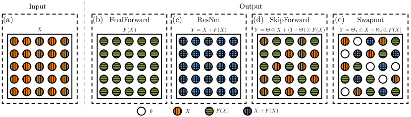
Dropout kills individual units randomly; stochastic depth skips entire blocks of units randomly. Swapout allows individual units to be dropped, or to skip blocks randomly. Implementing swapout is a straightforward generalization of dropout. Let be the input to some network block that computes . The ’th unit produces as output. Let be a tensor of i.i.d. Bernoulli random variables. Dropout computes the output of that block as
| (1) |
It is natural to think of dropout as randomly selecting an output from the set for the ’th unit.
Swapout generalizes dropout by expanding the choice of . Now write for distinct tensors of iid Bernoulli random variables indexed by and with corresponding parameters . Let be corresponding tensors consisting of values already computed somewhere in the network. Note that one of these can be itself (identity). However, are not restricted to being a function of and we drop the to indicate this. Most natural choices for are the outputs of earlier layers. Swapout computes the output of the layer in question by computing
| (2) |
and so, for unit , we have . We study the simplest case where
| (3) |
so that, for unit , we have . Thus, each unit in the layer could be:
- 1)
-
dropped (choose );
- 2)
-
a feedforward unit (choose );
- 3)
-
skipped (choose );
- 4)
-
or a residual network unit (choose ).
Since a swapout network can clearly imitate a residual network, and since residual networks are currently the best-performing networks on various standard benchmarks, we perform exhaustive experimental comparisons with them.
If one accepts the view of dropout and stochastic depth as averaging over a set of architectures, then swapout extends the set of architectures used. Appropriate random choices of and yield: all architectures covered by dropout; all architectures covered by stochastic depth; and block level skip connections. But other choices yield unit level skip and residual connections.
Swapout retains important properties of dropout. Swapout discourages co-adaptation by dropping units, but also by on occasion presenting units with inputs that have come from earlier layers. Dropout has been shown to enhance the stability of stochastic gradient descent ([3], lemma 4.4). This applies to swapout in its most general form, too. We extend the notation of that paper, and write for a Lipschitz constant that applies to the network, for the gradient of the network with parameters , and for the gradient of the dropped out version of the network.
The crucial point in the relevant enabling lemma is that (the inequality implies improvements). Now write for the gradient of a swapout network, and for the gradient of the swapout network which achieves the largest Lipschitz constant by choice of (this exists, because is discrete). First, a Lipschitz constant applies to this network; second, , so swapout makes stability no worse; third, we speculate light conditions on should provide , improving stability ([3] Section 4).
3.1 Inference in Stochastic Networks
A model trained with swapout represents an entire family of networks with tied parameters, where members of the family were sampled randomly during training. There are two options for inference. We could either replace random variables with their expected values, as recommended by Srivastava et al. [17] (deterministic inference). Alternatively, we could sample several members of the family at random, and average their predictions (stochastic inference).
There is an important difference between swapout and dropout. In a dropout network, one can estimate expectations exactly (as long as the network isn’t trained with batch normalization, below). This is because (recall is a tensor of Bernoulli random variables, and thus non-negative).
In a swapout network, one usually can not estimate expectations exactly. The problem is that is not the same as in general. Estimates of expectations that ignore this are successful, as the experiments show, but stochastic inference gives significantly better results.
Srivastava et al. argue that deterministic inference is significantly less expensive in computation. We believe that Srivastava et al. may have overestimated how many samples are required for an accurate average, because they use distinct dropout networks in the average (Figure 11 in [17]). Our experience of stochastic inference with swapout has been positive, with the number of samples needed for good behavior small (Figure 2). Furthermore, computational costs of inference are smaller when each instance of the network uses the same parameters
A technically more delicate point is that both dropout and swapout networks interact poorly with batch normalization if one uses deterministic inference. The problem is that the estimates collected by batch normalization during training may not reflect test time statistics. To see this consider two random variables and and let . While , it can be shown that with equality holding only for and . Thus, the variance estimates collected by Batch Normalization during training do not represent the statistics observed during testing if the expected values of and are used in a deterministic inference scheme. These errors in scale estimation accumulate as more and more layers are stacked. This may explain why [6] reports that dropout doesn’t lead to any improvement when used in residual networks with batch normalization.
3.2 Baseline comparison methods
ResNets:
Dropout:
Layer Dropout:
We replace equation 3 by . Here is a single Bernoulli random variable shared across all units.
SkipForward:
Equation 3 introduces two stochastic parameters and . We also explore and compare with a simpler architecture, SkipForward, that introduces only one parameter but samples from a smaller set as below.
| (4) |
4 Experiments
We experiment extensively on the CIFAR-10 dataset and demonstrate that a model trained with swapout outperforms a comparable ResNet model. Further, a 32 layer wider model matches the performance of a 1001 layer ResNet on both CIFAR-10 and CIFAR-100 datasets.
Model:
We experiment with ResNet architectures as described in [4](referred to as v1) and in [5](referred to as v2). However, our implementation (referred to as ResNet Ours) has the following modifications which improve the performance of the original model (Table 1). Between blocks of different feature sizes we subsample using average pooling instead of strided convolutions and use projection shortcuts with learned parameters. For final prediction we follow a scheme similar to Network in Network [11]. We replace average pooling and fully connected layer by a 1x1 convolution layer followed by global average pooling to predict the logits that are fed into the softmax.
Layers in ResNets are arranged in three groups with all convolutional layers in a group containing equal number of filters. We represent the number of filters in each group as a tuple with the smallest size as (16, 32, 64) (as used in [4]for CIFAR-10). We refer to this as width and experiment with various multiples of this base size represented as , etc.
Training:
We train using SGD with a batch size of 128, momentum of 0.9 and weight decay of 0.0001. Unless otherwise specified, we train all the models for a total 256 epochs. Starting from an initial learning rate of 0.1, we drop it by a factor of 10 after 196 epochs and then again after 224 epochs. We do the standard augmentation of left-right flips and random translations of up to four pixels. For translation, we pad the images by 4 pixels on all the sides and sample a random 32x32 crop. All the images in a mini-batch use the same crop. Note that dropout slows convergence ([17], A.4), and swapout should do so too for similar reasons. Thus using the same training schedule for all the methods should disadvantage swapout.
| Method | Width | #Params | Error(%) |
|---|---|---|---|
| ResNet v1 [4] | 0.27M | 8.75 | |
| ResNet v1 Ours | 0.27M | 8.54 | |
| Swapout v1 | 0.27M | 8.27 | |
| ResNet v2 Ours | 0.27M | 8.27 | |
| Swapout v2 | 0.27M | 7.97 | |
| Swapout v1 | 1.09M | 6.58 | |
| ResNet v2 Ours | 1.09M | 6.54 | |
| Stochastic Depth v2 Ours | 1.09M | 5.99 | |
| Dropout v2 | 1.09M | 5.87 | |
| SkipForward v2 | 1.09M | 6.11 | |
| Swapout v2 | 1.09M | 5.68 |
| Method | Deterministic Error(%) | Stochastic Error(%) |
|---|---|---|
| Swapout () | 10.36 | 6.69 |
| Swapout () | 10.14 | 7.63 |
| Swapout () | 7.58 | 6.56 |
| Swapout ( Linear(0.5, 1)) | 7.34 | 6.52 |
| Swapout ( Linear(1, 0.5)) | 6.43 | 5.68 |
Models trained with Swapout consistently outperform baselines:
Table 1 compares Swapout with various 20 layer baselines. Models trained with Swapout consistently outperform all other models of similar architecture.
The stochastic training schedule matters:
Different layers in a swapout network could be trained with different parameters of their Bernoulli distributions (the stochastic training schedule). Table 2 shows that different stochastic training schedules have a significant affect on the performance. We report the performance with deterministic as well as stochastic inference. These schedules differ in how the values of parameters and of the Bernoulli random variables in equation 3 are set for the different layers. Note that corresponds to the maximum stochasticity. A schedule with less randomness in the early layers (bottom row) performs the best. This is expected because Swapout adds per unit noise and early layers have the largest number of units. Thus, low stochasticity in early layers significantly reduces the randomness in the system. We use this schedule for all the experiments unless otherwise stated.
Swapout improves over ResNet architecture:
From Table 3 it is evident that networks trained with Swapout consistently show better performance than corresponding ResNets, for most choices of width investigated, using just the deterministic inference. This difference indicates that the performance improvement is not just an ensemble effect.
Stochastic inference outperforms deterministic inference:
Table 3 shows that the stochastic inference scheme outperforms the deterministic scheme in all the experiments. Prediction for each image is done by averaging the results of 30 stochastic forward passes. This difference is not just due to the widely reported effect that an ensemble of networks is better as networks in our ensemble share parameters. Instead, stochastic inference produces more accurate expectations and interacts better with batch normalization.
Stochastic inference needs few samples for a good estimate:
Increase in width leads to considerable performance improvements:
The number of filters in a convolutional layer is its width. Table 3 shows that the performance of a 20 layer model improves considerably as the width is increased both for the baseline ResNet v2 architecture as well as the models trained with Swapout. Swapout is better able to use the available capacity than the corresponding ResNet with similar architecture and number of parameters. Table 4 compares models trained with Swapout with other approaches on CIFAR-10 while Table 5 compares on CIFAR-100. On both datasets our shallower but wider model compares well with 1001 layer ResNet model.
Swapout uses parameters efficiently:
Experiments on CIFAR-100 confirm our results:
Table 5 shows that Swapout is very effective as it improves the performance of a 20 layer model (ResNet Ours) by more than 2%. Widening the network and reducing the stochasticity leads to further improvements. Further, a wider but relatively shallow model trained with Swapout (22.72%; 7.46M params) is competitive with the best performing, very deep (1001 layer) latest ResNet model (22.71%;10.2M params).
| Model | Width | #Params | ResNet v2 | Swapout | |
|---|---|---|---|---|---|
| Deterministic | Stochastic | ||||
| Swapout v2 (20) | (16, 32, 64) | 0.27M | 8.27 | 8.58 | 7.92 |
| Swapout v2 (20) | (32, 64, 128) | 1.09M | 6.54 | 6.40 | 5.68 |
| Swapout v2 (20) | (64, 128, 256) | 4.33M | 5.62 | 5.43 | 5.09 |
| Swapout v2 (32) | (64, 128, 256) | 7.43M | 5.23 | 4.97 | 4.76 |
| Method | #Params | Error(%) |
| DropConnect [20] | - | 9.32 |
| NIN [11] | - | 8.81 |
| FitNet(19) [15] | - | 8.39 |
| DSN [10] | - | 7.97 |
| Highway[18] | - | 7.60 |
| ResNet v1(110) [4] | 1.7M | 6.41 |
| Stochastic Depth v1(1202) [6] | 19.4M | 4.91 |
| SwapOut v1(20) | 1.09M | 6.58 |
| ResNet v2 (1001) [5] | 10.2M | 4.92 |
| SwapOut v2(32) | 7.43M | 4.76 |
| Method | Error(%) | |
|---|---|---|
| NIN [11] | - | 35.68 |
| DSN [10] | - | 34.57 |
| FitNet [15] | - | 35.04 |
| Highway [18] | - | 32.39 |
| ResNet v1 (110) [4] | 1.7M | 27.22 |
| Stochastic Depth v1 (110) [6] | 1.7M | 24.58 |
| ResNet v2 (164) [5] | 1.7M | 24.33 |
| ResNet v2 (1001) [5] | 10.2M | 22.71 |
| ResNet v2 Ours (20) | 1.09M | 28.08 |
| SwapOut v2 (20)(Linear(1,0.5)) | 1.10M | 25.86 |
| SwapOut v2 (56)(Linear(1,0.5)) | 3.43M | 24.86 |
| SwapOut v2 (56)(Linear(1,0.8)) | 3.43M | 23.46 |
| SwapOut v2 (32)(Linear(1,0.8)) | 7.46M | 22.72 |
5 Discussion and future work
Swapout is a stochastic training method that shows reliable improvements in performance and leads to networks that use parameters efficiently. Relatively shallow swapout networks give comparable performance to extremely deep residual networks.
We have shown that different stochastic training schedules produce different behaviors, but have not searched for the best schedule in any systematic way. It may be possible to obtain improvements by doing so. We have described an extremely general swapout mechanism. It is straightforward using equation 2 to apply swapout to inception networks [19] (by using several different functions of the input and a sufficiently general form of convolution); to recurrent convolutional networks [13] (by choosing to have the form ); and to gated networks. All our experiments focus on comparisons to residual networks because these are the current top performers on CIFAR-10 and CIFAR-100. It would be interesting to experiment with other versions of the method.
As with dropout and batch normalization, it is difficult to give a crisp explanation of why swapout works. We believe that our results support the idea that swapout causes some form of improvement in the optimization process. This is because relatively shallow networks with swapout reliably work as well as or better than quite deep alternatives; and because swapout is notably and reliably more efficient in its use of parameters than comparable deeper networks. Unlike dropout, swapout will often propagate gradients while still forcing units not to co-adapt. Furthermore, our swapout networks involve some form of tying between layers. When a unit sometimes sees layer and sometimes layer , the gradient signal will be exploited to encourage the two layers to behave similarly. The reason swapout is successful likely involves both of these points.
Acknowledgments:
This work is supported in part by ONR MURI Awards N00014-10-1-0934 and N00014-16-1-2007. We would like to thank NVIDIA for donating some of the GPUs used in this work.
References
- [1] Y. Bengio and O. Delalleau. On the expressive power of deep architectures. In Proceedings of the 22nd International Conference on Algorithmic Learning Theory, 2011.
- [2] X. Glorot, A. Bordes, and Y. Bengio. Deep sparse rectifier neural networks. In AISTATS, 2011.
- [3] M. Hardt, B. Recht, and Y. Singer. Train faster, generalize better: Stability of stochastic gradient descent. CoRR, abs/1509.01240, 2015.
- [4] K. He, X. Zhang, S. Ren, and J. Sun. Deep residual learning for image recognition. CoRR, abs/1512.03385, 2015.
- [5] K. He, X. Zhang, S. Ren, and J. Sun. Identity mappings in deep residual networks. CoRR, abs/1603.05027, 2016.
- [6] G. Huang, Y. Sun, Z. Liu, D. Sedra, and K. Q. Weinberger. Deep networks with stochastic depth. CoRR, abs/1603.09382, 2016.
- [7] S. Ioffe and C. Szegedy. Batch normalization: Accelerating deep network training by reducing internal covariate shift. CoRR, abs/1502.03167, 2015.
- [8] A. Krizhevsky, I. Sutskever, and G. E. Hinton. Imagenet classification with deep convolutional neural networks. In NIPS, 2012.
- [9] Y. LeCun, L. Bottou, Y. Bengio, and P. Haffner. Gradient-based learning applied to document recognition. Proceedings of the IEEE, 1998.
- [10] C.-Y. Lee, S. Xie, P. Gallagher, Z. Zhang, and Z. Tu. Deeply-supervised nets. AISTATS, 2015.
- [11] M. Lin, Q. Chen, and S. Yan. Network in network. CoRR, abs/1312.4400, 2013.
- [12] V. Nair and G. E. Hinton. Rectified linear units improve restricted boltzmann machines. In ICML, 2010.
- [13] P. H. Pinheiro and R. Collobert. Recurrent convolutional neural networks for scene parsing. arXiv preprint arXiv:1306.2795, 2013.
- [14] A. Rahimi and B. Recht. Random features for large-scale kernel machines. In NIPS, 2007.
- [15] A. Romero, N. Ballas, S. E. Kahou, A. Chassang, C. Gatta, and Y. Bengio. Fitnets: Hints for thin deep nets. ICLR, 2015.
- [16] K. Simonyan and A. Zisserman. Very deep convolutional networks for large-scale image recognition. CoRR, abs/1409.1556, 2014.
- [17] N. Srivastava, G. Hinton, A. Krizhevsky, I. Sutskever, and R. Salakhutdinov. Dropout: A simple way to prevent neural networks from overfitting. The Journal of Machine Learning Research, 2014.
- [18] R. K. Srivastava, K. Greff, and J. Schmidhuber. Training very deep networks. In NIPS, 2015.
- [19] C. Szegedy, W. Liu, Y. Jia, P. Sermanet, S. E. Reed, D. Anguelov, D. Erhan, V. Vanhoucke, and A. Rabinovich. Going deeper with convolutions. CoRR, abs/1409.4842, 2014.
- [20] L. Wan, M. Zeiler, S. Zhang, Y. L. Cun, and R. Fergus. Regularization of neural networks using dropconnect. In ICML, pages 1058–1066, 2013.
- [21] M. D. Zeiler and R. Fergus. Stochastic pooling for regularization of deep convolutional neural networks. arXiv preprint arXiv:1301.3557, 2013.