Two-Qubit Separability Probabilities as Joint Functions of the Bloch Radii of the Qubit Subsystems

Abstract

We detect a certain pattern of behavior of separability probabilities $p(r_{A},r_{B})$ for two-qubit systems endowed with Hilbert-Schmidt, and more generally, random induced measures, where $r_{A}$ and $r_{B}$ are the Bloch radii ($0\leq r_{A},r_{B}\leq 1$) of the qubit reduced states ($A,B$). We observe a relative repulsion of radii effect, that is $p(r_{A},r_{A})<p(r_{A},1-r_{A})$, except for rather narrow “crossover” intervals $[\tilde{r}_{A},\frac{1}{2}]$. Among the seven specific cases we study are, firstly, the “toy” seven-dimensional $X$-states model and, then, the fifteen-dimensional two-qubit states obtained by tracing over the pure states in $4\times K$-dimensions, for $K=3,4,5$, with $K=4$ corresponding to Hilbert-Schmidt (flat/Euclidean) measure. We also examine the real (two-rebit) $K=4$, the $X$-states $K=5$, and Bures (minimal monotone)–for which no nontrivial crossover behavior is observed–instances. In the two $X$-states cases, we derive analytical results; for $K=3,4$, we propose formulas that well-fit our numerical results; and for the other scenarios, rely presently upon large numerical analyses. The separability probability crossover regions found expand in length (lower $\tilde{r}_{A}$) as $K$ increases. This report continues our efforts (arXiv:1506.08739) to extend the recent work of Milz and Strunz (J. Phys. A: 48 [2015] 035306) from a univariate ($r_{A}$) framework—in which they found separability probabilities to hold constant with $r_{A}$—to a bivariate ($r_{A},r_{B}$) one. We also analyze the two-qutrit and qubit-qutrit counterparts reported in arXiv:1512.07210 in this context, and study two-qubit separability probabilities of the form $p(r_{A},\frac{1}{2})$. A physics.stack.exchange link to a contribution by Mark Fischler addressing, in considerable detail, the construction of suitable bivariate distributions is indicated at the end of the paper.

I Introduction

“The Bloch sphere provides a simple representation for the state space of the most primitive quantum unit–the qubit–resulting in geometric intuitions that are invaluable in countless fundamental information-processing scenarios” Jevtic et al. (2014).

Motivated by recent interesting work of Milz and Strunz Milz and Strunz (2015), indicating the constancy of Hilbert-Schmidt two-qubit (and qubit-qutrit) separability probabilities over the Bloch radius of qubit subsystems, we began a study in Slater (2015) devoted to extending their “single-Bloch radius” ($r_{A}$) results to “joint-Bloch-radii” ($r_{A},r_{B}$) analyses (cf. Gamel (2016)). Most of the many results/figures reported in Slater (2015) were based on extensive numerical investigations. However, a set of exact results was obtained for the “toy” model of $X$-states Mendonça et al. (2014), that is X-patterned $4\times 4$ density matrices having zero values at the eight entries–(1,2), (1,3), (2,1), (2,4), (3,1), (3,4), (4,2) and (4,3).

Milz and Strunz had found numerically-based evidence that the Hilbert-Schmidt (HS) volumes of the fifteen-dimensional convex sets of two-qubit systems and of their separable subsystems were both proportional to $(1-r_{A}^{2})^{6}$ (Milz and Strunz, 2015, eqs. (23), (30),(31)). The consequent constant ratio (separability probability) of the two (simply proportional) volume functions appeared to be $\frac{8}{33}$–a remarkably simple value for which a large body of diverse support had already been developed Slater (2007); Slater and Dunkl (2012); Slater (2013); Fei and Joynt ; Slater and Dunkl (2015a); Khvedelidze and Rogojin (2015) (Fonseca-Romero et al., 2012, sec. VII) (Shang et al., 2015, sec. 4), though yet no formal proof. (Let us note, however, that Lovas and Andai have recently reported substantial advances in this direction. They proved the $\frac{29}{64}$ two-rebit counterpart conjecture, and presented “an integral formula…which hopefully will help to prove the $\frac{8}{33}$ result” Lovas and Andai (2016).)

II $X$-states analyses

II.1 Hilbert-Schmidt ($K=4$) case

For the $X$-states, occupying a seven-dimensional subspace of the full fifteen-dimensional space, it was possible for Milz and Strunz to formally demonstrate that the counterpart total and separable volume functions, similarly, were both again proportional, but now to $(1-r_{A}^{2})^{3}$ (the square root of the fifteen-dimensional result). The corresponding constant (but at the isolated pure states [$r_{A}=1$] boundary) HS separability probability was greater than $\frac{8}{33}$, that is $\frac{2}{5}$ (Milz and Strunz, 2015, Apps. A, B). This $\frac{2}{5}$ result was also subsequently proven in Slater and Dunkl (2015b), along with companion $X$-states findings for the broader class of random induced measures Życzkowski and Sommers (2001); Aubrun et al. (2014); Adachi et al. (2009). (A distinct analytical approach, based on the Cholesky decomposition of density matrices, was utilized.)

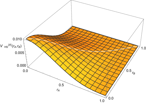
Figure 1: Bivariate Hilbert-Schmidt volume distribution (2) for the $X$-state model

In Slater (2015), we employed the $X$-states parametrization and transformations indicated by Braga, Souza and Mizrahi (Braga et al., 2010, eqs. (6), (7)). We were able to reproduce the Hilbert-Schmidt univariate volume result of Milz and Strunz (Milz and Strunz, 2015, eq. (20), Fig. 1) Slater and Dunkl (2015b),

$$V^{(X)}_{HS}(r)=\frac{\pi^{2}}{2304}(1-r^{2})^{3},$$ (1)

as the marginal distribution (over either $r_{A}$ or $r_{B}$) of the bivariate distribution (Fig. 1),

$$_{{tot}}V^{(X)}_{HS}(r_{A},r_{B})=$$ (2)

$$\begin{cases}-\frac{1}{960}\pi^{2}\left(r_{A}-1\right){}^{3}\left(r_{A}\left(r_{A}+3\right)-5r_{B}^{2}+1\right)&r_{A}>r_{B}\\ -\frac{1}{960}\pi^{2}\left(r_{B}-1\right){}^{3}\left(-5r_{A}^{2}+r_{B}\left(r_{B}+3\right)+1\right)&r_{A}<r_{B}\end{cases}.$$

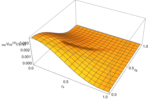
Figure 2: Bivariate Hilbert-Schmidt separable volume distribution (3) for the $X$-state model

To, then, obtain the desired $X$-states bivariate separability probability distribution $p^{(X)}_{HS}(r_{A},r_{B})$, we further found the separable volume counterpart to (2) (Fig. 2),

$$_{{sep}}V^{(X)}_{HS}(r_{A},r_{B})=$$ (3)

$$\begin{cases}-\frac{\pi^{2}\left(r_{A}-1\right){}^{3}\left(5\left(r_{A}+3\right)r_{B}^{4}-10\left(3r_{A}+1\right)r_{B}^{2}+8r_{A}^{2}+9r_{A}+3\right)}{7680}&r_{A}>r_{B}\\ -\frac{\pi^{2}\left(r_{B}-1\right){}^{3}\left(5r_{A}^{4}\left(r_{B}+3\right)-10r_{A}^{2}\left(3r_{B}+1\right)+r_{B}\left(8r_{B}+9\right)+3\right)}{7680}&r_{A}<r_{B}\end{cases},$$

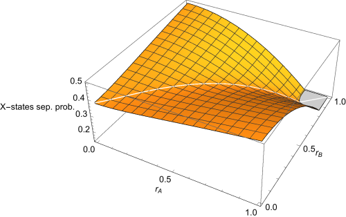
Figure 3: Bivariate Hilbert-Schmidt separability probability distribution (4)–the ratio of Fig. 2 to Fig. 1–for the $X$-state model

and took their ratio (Fig. 3) (note the cancellation of the $(r-1)^{3}$-type factors),

$$p^{(X)}_{HS}(r_{A},r_{B})=\frac{{}_{{sep}}V^{(X)}_{HS}(r_{A},r_{B})}{{}_{{tot}}V^{(X)}_{HS}(r_{A},r_{B})}=$$ (4)

$$\begin{cases}\frac{5\left(r_{A}+3\right)r_{B}^{4}-10\left(3r_{A}+1\right)r_{B}^{2}+8r_{A}^{2}+9r_{A}+3}{8\left(r_{A}\left(r_{A}+3\right)-5r_{B}^{2}+1\right)}&r_{A}>r_{B}\\ \frac{5r_{A}^{4}\left(r_{B}+3\right)-10r_{A}^{2}\left(3r_{B}+1\right)+r_{B}\left(8r_{B}+9\right)+3}{8\left(-5r_{A}^{2}+r_{B}\left(r_{B}+3\right)+1\right)}&r_{A}<r_{B}\end{cases}.$$

(Numerical integration of this function over $[0,1]^{2}$ yielded $0.381678\approx 0.4$–so, it would seem that $p^{(X)}_{HS}(r_{A},r_{B})$ is not strictly a scaled version of a doubly-stochastic measure Sungur and Ng (2005); Ruschendorf et al. (1996), as we had speculated it might be.)

Fig. 4 (also (Slater, 2015, Fig. 50)) shows the (largely lower) $r_{A}=r_{B}$ and (largely upper) $r_{A}+r_{B}=1$ one-dimensional cross-sections of Fig. 3. (We computed the correlation between $r_{A}$ and $r_{B}$ to be $1-\frac{11206656}{37748736-10080\pi^{2}+\pi^{4}}\approx 0.702341$ for all states and only slightly less, $1-\frac{74649600}{235929600-25200\pi^{2}+\pi^{4}}\approx 0.68326$, for the separable $X$-states (cf. de Vicente ).) In Fig. 5 we show more closely the crossover region in which the $p^{(X)}_{HS}(r_{A},1-r_{A})$ curve becomes dominated by the $p^{(X)}_{HS}(r_{A},r_{A})$ curve.

The analytic form of the $r_{A}=r_{B}$ $X$-states separability probability curve is

$$p^{(X)}_{HS}(r_{A},r_{A})=-\frac{(r_{A}-1)(5r_{A}(r_{A}(r_{A}+5)+3)+3)}{32r_{A}+8}.$$ (5)

At particular points of interest, we have $p^{(X)}_{HS}(\frac{1}{2},\frac{1}{2})=\frac{139}{384}=\frac{139}{2^{7}\cdot 3}$, $p^{(X)}_{HS}(0,0)=\frac{3}{8}$, and $p^{(X)}_{HS}(1,1)=0$. The maximum of $p^{(X)}_{HS}(r_{A},r_{A})$ is achieved at the positive root ($r_{A}\approx 0.2722700792$) of the cubic equation $3r_{A}^{3}+9r_{A}^{2}+r_{A}-1=0$. Its value ($\approx 0.393558399$) there is the positive root of the cubic equation $54r_{A}^{3}+108r_{A}^{2}-28r_{A}-9=0$.

On the other hand, the minimum of the $r_{A}+r_{B}=1$ (“antidiagonal”) curve

$$p^{(X)}_{HS}(r_{A},1-r_{A})=\begin{cases}-\frac{(r_{A}-2)r_{A}\left(5r_{A}\left(r_{A}^{2}+r_{A}-10\right)+28\right)+8}{8(r_{A}(4r_{A}-13)+4)}&2r_{A}>1\\ \frac{r_{A}(r_{A}(5r_{A}((r_{A}-4)r_{A}-6)+32)+25)-20}{8(r_{A}(4r_{A}+5)-5)}&2r_{A}<1\end{cases}$$ (6)

is, again, $\frac{139}{384}$, clearly attained at the point of symmetry, $r_{A}=\frac{1}{2}$. (We employ the terms ”diagonal” and ”antidiagonal” to describe the two types of curves under investigation, in reference to the entries of the $100\times 100$ data matrices we employ for their estimation.) Also, at the endpoints,

$$p^{(X)}_{HS}(0,1)=p^{(X)}_{HS}(1,0)=\frac{1}{2}$$ (7)

are the two maxima of $p^{(X)}_{HS}(r_{A},1-r_{A})$.

We note–in line with our general observations throughout the paper–that in the crossover region $r_{A}\in[0.40182804,\frac{1}{2}]$ (Figs. 4 and 5), the $p^{(X)}_{HS}(r_{A},1-r_{A})$ curve changes from dominating the $p^{(X)}_{HS}(r_{A},r_{A})$ curve to being subordinate to it–so that the radii are relatively “attractive” and not relatively “repulsive” in this domain. The lower bound of the region $\tilde{r}_{A}=0.40182804$ is a root of the quintic equation (with remarkably simple coefficients)

$$4r_{A}^{5}+5r_{A}^{4}-8r_{A}^{3}-14r_{A}^{2}+4r_{A}+1=0.$$ (8)

The maximum gap of 0.0056796160 between the two curves in the crossover region is attained at $r_{A}=0.4564893379$.

II.2 Random induced ($K=5$) case

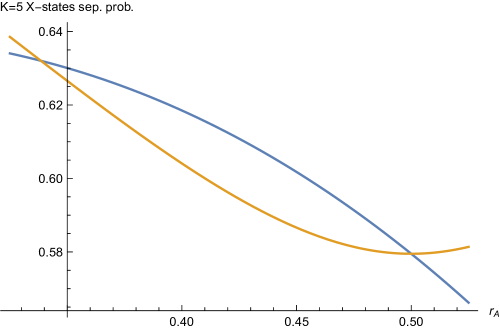
Figure 6: Crossover region for the random induced $K=5$ $X$-states case, the lower intersection point of the crossover region being $\tilde{r}_{A}=0.3385355079$, a root of the eighth-degree equation (9)

Exact total and separable volume and (consequent) separability probability formulas have been reported (Slater, 2015, sec. IX.D) also for the $X$-states random induced $K=5$ counterpart. (The marginal total and separable volumes are now both proportional to $(1-r_{A}^{2})^{5}$.) In Fig. 6 we show the (more pronounced) crossover behavior in that scenario. The lower crossover point of $\tilde{r}_{A}=0.3385355079$ is a root of the eighth-degree equation (with rather simple well-behaved coefficients–all divisible by 7, but for 27)

$$112r_{A}^{8}+252r_{A}^{7}-203r_{A}^{6}-938r_{A}^{5}-441r_{A}^{4}+728r_{A}^{3}+27r_{A}^{2}-42r_{A}-7=0.$$ (9)

Consistently with our general observations below, this lower boundary $\tilde{r}_{A}=0.3385355079$ of the crossover region is smaller than that reported above (eq. (8)), $\tilde{r}_{A}=0.40182804$, in the Hilbert-Schmidt ($K=4<5$) $X$-states scenario.

III Full two-qubit and two-rebit analyses

Now, let us transition from studying these two seven-dimensional $X$-states examples, to five–$K=3,4,5$, rebit, and Bures cases–for the full fifteen-dimensional two-qubit states. In all these cases we generated corresponding sets of random density matrices, and discretized the values of the two Bloch radii found into intervals of length $\frac{1}{100}$, obtaining thereby $100\times 100$ data matrices of separable and total counts.

III.1 Random induced ($K=3)$ case

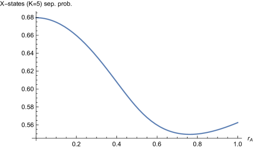
Figure 17: Plot of $p^{(X)}_{K=5}(r_{A},\frac{1}{2})$ given by (27)

Firstly, we study the instance when this set is endowed with the $K=3$ instance of random induced measure Życzkowski and Sommers (2001); Bengtsson and Życzkowski (2006); Adachi et al. (2009). (The corresponding [overall] separability probability, then, appears to be $\frac{1}{14}\approx 0.0714286$ (Slater and Dunkl, 2015b, eq. (2)) (Slater, 2015, Fig. 17).). The (apparent, well-fitting) total volume formula we obtained, after extensive investigations, was

$$_{{tot}}V_{K=3}(r_{A},r_{B})=\begin{cases}\frac{8\left(r_{A}-1\right){}^{4}\left(r_{A}^{2}+4r_{A}-5r_{B}^{2}\right)}{r_{A}}&0<r_{B}<r_{A}<1\\ \frac{8\left(r_{B}-1\right){}^{4}\left(r_{B}\left(r_{B}+4\right)-5r_{A}^{2}\right)}{r_{B}}&0<r_{A}<r_{B}<1\\ -32\left(r_{A}-1\right){}^{5}&r_{B}=r_{A}\end{cases},$$ (10)

choosing to normalize so that ${}_{{tot}}V_{(K=3)}(\frac{1}{2},\frac{1}{2})=1$.

Further, for $r_{B}=r_{A}$, we appear to have

$$_{{sep}}V_{K=3}(r_{A},r_{A})=\left(r_{A}-1\right){}^{6}\left(r_{A}^{2}+6r_{A}+1\right),$$ (11)

so that, by taking a ratio, we obtain the diagonal curve

$$p_{K=3}(r_{A},r_{A})=\frac{1}{32}\left(1-r_{A}\right)\left(r_{A}^{2}+6r_{A}+1\right).$$ (12)

For $0<r_{B}<r_{A}<1$,

$$_{{sep}}V_{K=3}(r_{A},r_{B})=$$ (13)

$$-\frac{\left(r_{A}-1\right){}^{4}\left(-r_{A}^{3}\left(6012r_{B}+2351\right)+2r_{A}^{2}\left(2424r_{B}-9859\right)+Tr_{A}+2785r_{A}^{4}+Sr_{B}\right)}{5100r_{A}}$$

with

$$S=-22675r_{B}^{3}-852r_{B}^{2}+470r_{B}+96;\hskip 21.68121ptT=-5100r_{B}^{4}+5502r_{B}^{3}+49355r_{B}^{2}-1152r_{B}-5196.$$

The $0<r_{A}<r_{B}<1$ component of this piecewise function ${}_{{sep}}V_{K=3}(r_{A},r_{B})$ can be obtained by interchanging the roles of $r_{A}$ and $r_{B}$ in (13). (These formulas [for which we lack formal proofs] were developed -with very considerable, diverse fitting efforts -using 10,962,000,000 randomly generated $4\times 4$ density matrices assigned $K=3$ measure, employing the Ginibre-matrix-based algorithm specified in Miszczak (2012) (cf. Miszczak (2013))).

The marginal distribution of the total volume function (10) over $r_{B}$ (cf. (Milz and Strunz, 2015, eq. (24))) is $\frac{4\pi}{3}\left(r_{A}^{2}-1\right){}^{4}$, and of the separable volume function, $\frac{2\pi}{21}\left(r_{A}^{2}-1\right){}^{4}$, giving us -taking their ratio -the constant separability probability for this scenario of $\frac{1}{14}=(\frac{2\pi}{21})/(\frac{4\pi}{3})$ (Slater and Dunkl, 2015b, eq. (2)) (Slater, 2015, Fig. 17).

Further, we have the antidiagonal function

$$p_{K=3}(r_{A},1-r_{A})=\begin{cases}\frac{5100r_{A}^{5}-24480r_{A}^{4}-66682r_{A}^{3}+49256r_{A}^{2}+38325r_{A}-24480}{40800\left(4r_{A}^{2}+6r_{A}-5\right)}&0<r_{A}<\frac{1}{2}\\ \frac{-5100r_{A}^{5}+1020r_{A}^{4}+113602r_{A}^{3}-246670r_{A}^{2}+135629r_{A}-22961}{40800\left(4r_{A}^{2}-14r_{A}+5\right)}&\frac{1}{2}<r_{A}<1\end{cases}.$$ (14)

Its maximum is attained at the two endpoints of [0,1] (cf. (7))

$$p_{K=3}(0,1)=p_{K=3}(1,0)=\frac{1}{2}.$$ (15)

Based upon these $K=3$ volume formulas ((10), (11)), we find, solving the quartic equation,

$$5100r_{A}^{4}+6885r_{A}^{3}-26711r_{A}^{2}-26340r_{A}+18105=0,$$ (16)

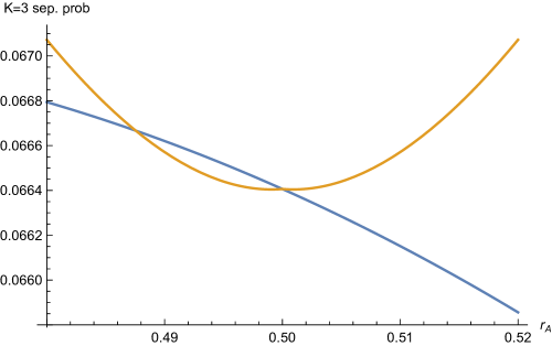
Figure 7: Crossover region for $K=3$, based upon the separability probability formulas ((12), (14)), with the lower intersection point of the crossover region being $\tilde{r}_{A}=0.48754$

that the lower boundary is $\tilde{r}_{A}=0.487543066126$, rather near to $r_{A}=\frac{1}{2}$. (Alternatively, interpolating the raw data, we obtain an estimate $\tilde{r}_{A}=0.488124$.) In Fig. 7 (cf. Fig. 5) we show this crossover region.

III.2 Hilbert-Schmidt ($K=4$) case

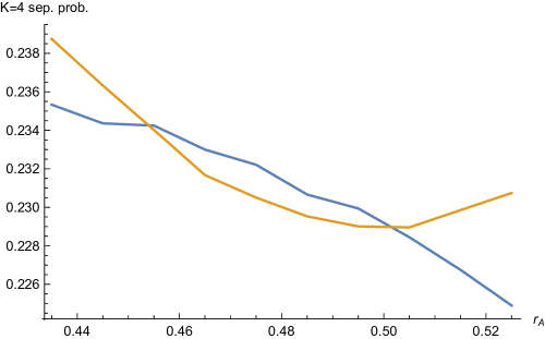
Figure 8: Crossover region for the Hilbert-Schmidt case $K=4$, based upon 13,800,000,000 randomly generated density matrices, with the sampled Bloch radii $r_{A},r_{B}\in[0,1]$ discretized into intervals of length $\frac{1}{100}$. Our estimate of the lower crossover point is $\tilde{r}_{A}=0.453893$. The maximum gap of 0.001708 between the two curves in the crossover region is attained at $r_{A}=0.474381$.

In Fig. 8, we show the crossover behavior for the fundamental Hilbert-Schmidt $K=4$ case. (To reiterate, a considerable body of strongly compelling evidence has been developed that the corresponding separability probability is $\frac{8}{33}\approx 0.242424$ Slater (2007); Slater and Dunkl (2012); Slater (2013); Fei and Joynt ; Slater and Dunkl (2015a); Khvedelidze and Rogojin (2015) (Fonseca-Romero et al., 2012, sec. VII) (Shang et al., 2015, sec. 4).)

Choosing again to normalize so that ${}_{{tot}}V^{K=4}_{HS}(\frac{1}{2},\frac{1}{2})=1$, it appears that

$${}_{{tot}}V^{K=4}_{HS}(r_{A},r_{A})=\frac{256}{5}\left(1-r_{A}\right){}^{8}\left(8r_{A}+1\right)$$ (17)

and

$${}_{{sep}}V^{K=4}_{HS}(r_{A},r_{A})=\frac{28}{3}\left(1-r_{A}\right){}^{9}\left(29r_{A}^{2}+\frac{17r_{A}}{2}+1\right),$$ (18)

so that, a fit to the diagonal curve can be obtained using

$$p^{K=4}_{HS}(r_{A},r_{A})=-\frac{35\left(r_{A}-1\right)\left(58r_{A}^{2}+17r_{A}+2\right)}{384\left(8r_{A}+1\right)}.$$ (19)

Further, for the antidiagonal curve, we have a close fit (using a chi-squared objective function) for the region $r_{A}\in[0,\frac{1}{2}]$ (the curve for $r_{A}\in[\frac{1}{2},1]$ can be obtained by replacing $r_{A}$ by $1-r_{A}$),

$$p^{K=4}_{HS}(r_{A},1-r_{A})\approx$$ (20)

$$\frac{-0.660807r_{A}^{6}-119.919r_{A}^{5}+237.198r_{A}^{4}-200.68r_{A}^{3}+90.0466r_{A}^{2}-21.6016r_{A}+2.32483}{-1.r_{A}^{4}-66.164r_{A}^{3}+75.933r_{A}^{2}-30.4436r_{A}+4.64965}.$$

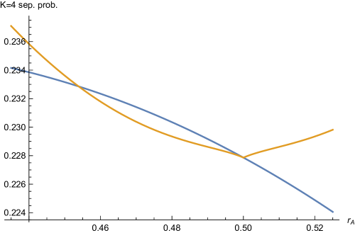
Figure 9: Predicted crossover region (cf. Fig. 8) for the Hilbert-Schmidt case $K=4$, based upon the formulas ((19), (20)) for $p^{K=4}_{HS}(r_{A},r_{A})$ and $p^{K=4}_{HS}(r_{A},1-r_{A})$

In Fig. 9, we show the predicted $K=4$ crossover region based on these last two formulas. (The marginal distributions of the total and separable $K=4$ volume functions over $r_{B}$ appear, as Milz and Strunz argued, to be both proportional to $\left(r_{A}^{2}-1\right){}^{6}$ (Milz and Strunz, 2015, eq. (23)), with the associated constant ratio being $\frac{8}{33}$.)

III.3 Random induced ($K=5$) case

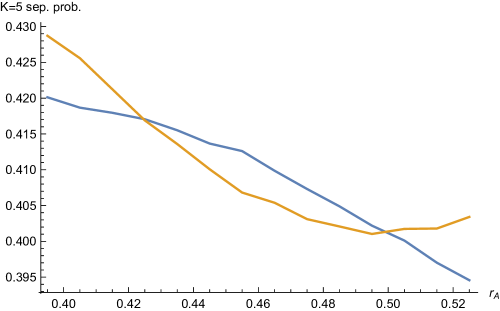
Figure 10: Crossover region for $K=5$, based upon 6,343,000,000 randomly generated density matrices, with the sampled Bloch radii $r_{A},r_{B}\in[0,1]$ discretized into intervals of length $\frac{1}{100}$. Our estimate of the lower crossover point is $\tilde{r}_{A}=0.424453$.

In Fig. 10 we show the results for the two-qubit random induced $K=5$ analysis. Normalizing again so that ${}_{{tot}}V_{K=5}(\frac{1}{2},\frac{1}{2})=1$, it appears that (Slater, 2015, sec. IV.B)

$${}_{{tot}}V_{K=5}(r_{A},r_{A})=\frac{4096}{33}\left(1-r_{A}\right){}^{11}\left(40r_{A}^{2}+11r_{A}+1\right).$$ (21)

A good fit can be obtained using

$${}_{{sep}}V_{K=5}(r_{A},r_{A})=49\left(1-r_{A}\right){}^{12}\left(108r_{A}^{3}+\frac{111r_{A}^{2}}{2}+10r_{A}+1\right),$$ (22)

so that

$$p_{K=5}(r_{A},r_{A})\approx-\frac{1617\left(r_{A}-1\right)\left(216r_{A}^{3}+111r_{A}^{2}+20r_{A}+2\right)}{8192\left(40r_{A}^{2}+11r_{A}+1\right)}.$$ (23)

The corresponding (overall) separability probability appears to be $\frac{61}{143}\approx 0.426573$ (Slater and Dunkl, 2015b, eq. (2), Table II) (Slater, 2015, Fig. 24), obtainable by taking the ratio of marginal separable and total volume functions, both proportional to $\left(r_{A}^{2}-1\right){}^{8}$. So, for $K=3,4,5$, we have the sequence ($2K-1$) of exponents of $\left(r_{A}^{2}-1\right){}$ of 4, 6 and 8 for the marginal distributions.

We see that, as a general rule, the lower bounds ($\tilde{r}_{A}$) to the crossover regions decrease as $K$ increases.

III.4 Two-rebit and Bures cases

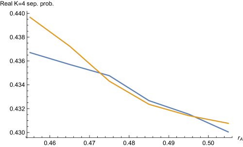
Figure 11: Crossover region for the Hilbert-Schmidt case $K=4$, based upon 3,928,000,000 randomly generated real (two-rebit) density matrices, with the sampled Bloch radii $r_{A},r_{B}\in[0,1]$ discretized into intervals of length $\frac{1}{100}$. Our estimate of the lower crossover point is $\tilde{r}_{A}=0.4722$.

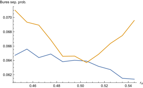
Figure 12: Joint plot of (lower) $p^{Bures}(r_{A},r_{A})$ and (upper) $p^{Bures}(r_{A},1-r_{A})$ curves based upon 424,000,000 randomly generated density matrices. The two curves appear to cross ever so slightly above $r_{A}=\frac{1}{2}$, so there is no evidence of significant crossover behavior in this setting.

In Slater (2015), we had also examined the nature of the separability probabilities $p(r_{A},r_{B})$ in the $K=4$ (Hilbert-Schmidt) “toy” case with the entries of the density matrix restricted to real values (forming a nine-dimensional -as opposed to fifteen-dimensional -convex set), and also for the two-qubit states endowed with Bures (minimal monotone) measure Sommers and Życzkowski (2003); Bengtsson and Życzkowski (2006). Based upon the samples of random density matrices generated there, we further observe (Fig. 11) crossover behavior (of a “thin” nature) in the former (two-re[al]bit) case, but, interestingly, none apparently (below $r_{A}=\frac{1}{2}$) in the Bures instance (Fig. 12). (Let us note that the Bures-based Fig. 31 in Slater (2015) showed highly convincingly that, in strong contrast to the use of Hilbert-Schmidt and random induced measures, the Bures separability probability rapidly decreases as $r_{A}$ increases, rather than remains constant, as for all the other scenarios discussed above.) So, we are inclined to believe that nontrivial crossover behavior is restricted to the use of Hilbert-Schmidt and associated random induced measures Życzkowski and Sommers (2001), and that the vague Bures crossover in Fig. 12 is purely an insignificant sampling phenomenon.

It very strongly appears in the two-rebit case–in contrast to the integral exponents otherwise so far observed–that both the total and separable volume marginal distributions are now proportional to $(1-r_{A}^{2})^{\frac{7}{2}}$ (with the consequent constant separability probability over $r_{A}$, being $\frac{29}{64}$ Slater (2013)).

IV The case of two-qutrits

IV.1 The role of Casimir invariants

Our focus here and in Slater (2015) has been on the extension of the two-qubit analyses of Milz and Strunz Milz and Strunz (2015)–in which they found separability probabilities to be constant over the (standard) Bloch radius of qubit subsystems–to a bivariate ($r_{A},r_{B}$) setting. In Slater (2016), we found evidence for another form of extension. It appears that Hilbert-Schmidt and more generally, random induced separability (and PPT [positive partial transpose]) probabilities are constant, additionally, over “generalized Bloch radii” (in group-theoretic terms, square roots of quadratic Casimir invariants) of qutrit subsystems Goyal et al. (2016). Further, constancies appear to continue to hold, as well, over cubic Casimir invariants (and, hypothetically, over quartic,…, ones) of reduced higher-dimensional (qudit) states.

IV.2 Hilbert-Schmidt Analysis

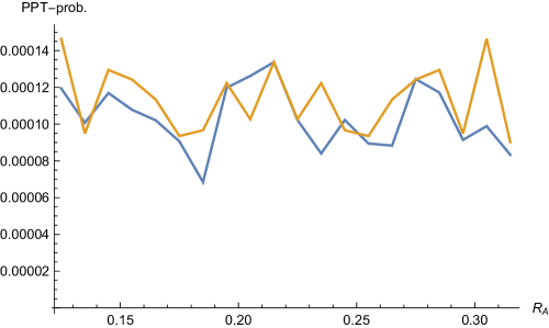
Figure 13: The largely dominant two-qutrit PPT-probability $p^{Qutrit}_{HS}(R_{A},0.435-R_{A})$, along with the largely subordinate $p^{Qutrit}_{HS}(R_{A},R_{A})$, based on one hundred million $9\times 9$ density matrices, randomly generated with respect to Hilbert-Schmidt ($K=9,N=9$) measure. A possible crossover region appears near $R_{A}=0.2$.

The question naturally arises of whether or not the various phenomena documented above in the case of two-qubit systems is also present in some analogous forms in two-qutrit systems, replacing the standard Bloch radiii ($r_{A},r_{B}$) with their generalized counterparts ($R_{A},R_{B}$). In (Slater, 2016, sec. III.A), one hundred million two-qutrit density matrices were generated, randomly with respect to Hilbert-Schmidt measure ($K=N=9$). (None of them had $R>0.58$.) Only 10,218 of them had positive partial transposes, with the associated generalized Bloch radii now all lying roughly between 0.05 and 0.44. In Fig. 13, we plot the largely dominant $p^{Qutrit}_{HS}(R_{A},0.435-R_{A})$ curve, along with the $p^{Qutrit}_{HS}(R_{A},R_{A})$ diagonal curve. There is a suggestion of a possible crossover region near $R_{A}=0.2$.

IV.3 Random induced ($K=24,N=9$) measure

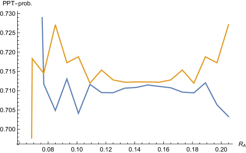
Figure 14: The dominant two-qutrit PPT-probability $p^{Qutrit}_{K=24}(R_{A},0.265-R_{A})$, along with the subordinate $p^{Qutrit}_{K=24}(R_{A},R_{A})$, based on 36,400,000 $9\times 9$ density matrices, randomly generated with respect to induced ($K=24,N=9$) measure. No crossover seems evident.

As a supplementary exercise—initially being concerned that the previous PPT-probability was too small to detect meaningful effects—we generated 36,400,000 two-qutrit density matrices, with respect to random induced ($K=24,N=9$) measure. The sample PPT-probability was now, orders of magnitude greater than 0.00010218, that is, 0.71179. In Fig.14, we plot the quasi-antidiagonal $p^{Qutrit}_{K=24}(R_{A},0.265-R_{A})$ and the diagonal $p^{Qutrit}_{K=24}(R_{A},R_{A})$ curves. We see no crossover behavior, noting the restricted range of values of $R_{A}$, beyond which no significant data were obtained. So, only generalized Bloch radii repulsion–and not attraction–is evident in this plot.

V The “hybrid” qubit-qutrit case

In (Slater, 2016, sec. II), we also conducted a qubit-qutrit analysis based upon one hundred million $6\times 6$ density matrices, randomly generated with respect to Hilbert-Schmidt ($K=N=6$) measure. Let us consider the $A$ subsystem there to be that of the reduced state qubit, and the $B$ subsystem to be that of the reduced state qutrit. Now, we are in a situation where we have no obvious reason to expect that the $100\times 100$ data matrix obtained by using “bins” of length $\frac{1}{100}$ for both $r_{A}$ and $R_{B}$ to tend to be symmetric in nature.

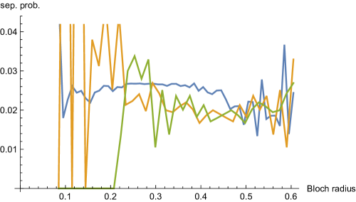
Figure 15: The most level (least jagged) of the three qubit-qutrit-based curves corresponds to the diagonal $p_{HS}^{QubQut}(r_{A},r_{A})=p_{HS}^{QubQut}(R_{B},R_{B})$ curve, the most jagged (highest) to the antidiagonal $p_{HS}^{QubQut}(1-R_{B},R_{B})$ curve and the intermediate one to the antidiagonal reversal $p_{HS}^{QubQut}(r_{A},1-r_{A})$.

In Fig. 15, we now plot three curves of interest. The smoothest in character corresponds to the “diagonal” case, when the qubit Bloch radius ($r_{A}$) is equal in magnitude (modulo bin size) to the qutrit generalized Bloch radius ($R_{B}$). The most jagged of the three curves is the antidiagonal $p_{HS}^{QubQut}(1-R_{B},R_{B})$ one, while the intermediate one, $p_{HS}^{QubQut}(r_{A},1-r_{A})$, is the reversal of that antidiagonal. The possibility appears of a crossover-type region between 0.3 and 0.5, in which the diagonal $r_{A}=R_{B}$ curve is dominant.

V.1 Further possible hybrid analyses

Additional “hybrid” analyses such as the qubit-qutrit one just described (sec. V) were reported in Slater (2016). These included a qubit-qudit ($8\times 8$ density matrix) analysis (Slater, 2016, sec. III.B), as well as two further qubit-qutrit studies. One of these two was based on random induced ($K=9,N=6$), rather than strictly Hilbert-Schmidt, measure (Slater, 2016, sec. VI). The other employed the cubic Casimir invariant (rather than the square root of the quadratic invariant–that is the qutrit generalized Bloch radius) (Slater, 2016, sec. IV.A). We might also pursue “crossover” investigations in these further hybrid settings. Then again, the $100\times 100$ data matrices that were generated (by “binning” the values of the two differing forms of Bloch radii recorded into intervals of length $\frac{1}{100}$) can not be expected to be fundamentally symmetric in character.

VI Two-Qubit ($r_{B}=\frac{1}{2}$) Analyses

Aside from the $X$-states $K=4$ (Hilbert-Schmidt) and $K=5$ analyses reported above (secs. II.1 and II.2), much work remains to place the other scenarios studied here and similar ones in a more formal, rigorous setting. Our results have concentrated on the relations (intersections,…) between “diagonal” and “antidiagonal” one-dimensional sections of bivariate distributions–themselves worthy of fuller understandings. Perhaps the form of one-dimensional section most natural/appealing to study, to yield more insights in addition to these two types, would, in the two-qubit context, be $p(r_{A},\frac{1}{2})$, that is setting $r_{B}=\frac{1}{2}$. We now briefly investigate this issue.

For our initially studied $X$-states $K=4$ (Hilbert-Schmidt) model (sec. II.1), we have the result

$$p^{(X)}_{HS}(r_{A},\frac{1}{2})=\begin{cases}\frac{35r_{A}^{4}-50r_{A}^{2}+19}{44-80r_{A}^{2}}&0<r_{A}<\frac{1}{2}\\ \frac{128r_{A}^{2}+29r_{A}+23}{32\left(4r_{A}^{2}+12r_{A}-1\right)}&\frac{1}{2}<r_{A}<1\\ \frac{139}{384}&r_{A}=r_{B}\end{cases}.$$ (24)

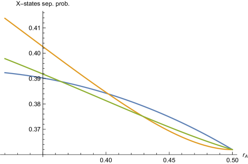
Figure 16: Joint plot for the $X$-states $K=4$ (Hilbert-Schmidt) two-qubit model of the three curves $p^{(X)}_{HS}(r_{A},\frac{1}{2})$, $p^{(X)}_{HS}(r_{A},r_{A})$ and $p^{(X)}_{HS}(r_{A},1-r_{A})$. The first of these three lies between the other two near $r_{A}=\frac{1}{2}$.

Expanding upon Figs. 4 and 5, in Fig. 16 we plot $p^{(X)}_{HS}(r_{A},\frac{1}{2})$, along with the previously jointly plotted $p^{(X)}_{HS}(r_{A},r_{A})$ and $p^{(X)}_{HS}(r_{A},1-r_{A})$. All three curves intersect obviously (by construction) at $r_{A}=\frac{1}{2}$. Additionally, the first two listed intersect at $r_{A}=0.364314$, a root of the quintic equation

$$10r_{A}^{5}+17r_{A}^{4}-24r_{A}^{3}-18r_{A}^{2}+6r_{A}+1=0,$$ (25)

and the first and the third at $r_{A}=0.428908$, a root of the sextic equation

$$10r_{A}^{6}-7r_{A}^{5}-34r_{A}^{4}-6r_{A}^{3}+30r_{A}^{2}+5r_{A}-6=0.$$ (26)

For the $X$-states $K=5$ model (sec. II.2) (Fig. 17), we have

$$p^{(X)}_{K=5}(r_{A},\frac{1}{2})=\begin{cases}\frac{-231r_{A}^{6}+441r_{A}^{4}-297r_{A}^{2}+70}{336r_{A}^{4}-360r_{A}^{2}+103}&0<r_{A}<\frac{1}{2}\\ \frac{512r_{A}^{4}+2560r_{A}^{3}-384r_{A}^{2}+679r_{A}+35}{32\left(16r_{A}^{4}+80r_{A}^{3}+120r_{A}^{2}-40r_{A}+13\right)}&\frac{1}{2}<r_{A}<1\\ \frac{1261}{2176}&r_{A}=r_{B}\end{cases}.$$ (27)

VII Concluding Remarks

If we examine the analytically-derived total and separable volume piecewise formulas ((2), (3)) for the $X$-states ($K=4$, Hilbert-Schmidt) “toy” model that we have employed as our starting point, we see that the pieces are bivariate polynomials in $r_{A}$ and $r_{B}$. On the other hand, the analogous pieces in the candidate (well-fitting) formulas ((10), (11)) we have advanced in the 15-dimensional $K=3$ case, are such polynomials divided by $r_{A}$ or $r_{B}$–that is, rational functions. A similar situation holds with regard to our working formulas for the 15-dimensional $K=4$ (Hilbert-Schmidt) scenario–which we have employed for our estimate (20) of $p^{K=4}_{HS}(r_{A},1-r_{A})$. This type of functional difference is a matter of some interest/concern, meriting further investigation. (The distinction between rational and polynomial functions, of course, disappears in the computation of the ratios yielding the separability probabilities.) These volume formulas were constructed so as to satisfy the marginal constraints $(1-r_{A}^{2})^{n}$, $n=2(K-1)$, $K=3,4$, with the resultant indicated proportionalities of $\frac{1}{14}$ and $\frac{8}{33}$, and also to satisfy the apparent diagonal separability probabilities (12) and (19) of $p_{K=3}(r_{A},r_{A})=\frac{1}{32}\left(1-r_{A}\right)\left(r_{A}^{2}+6r_{A}+1\right)$ and $p^{K=4}_{HS}(r_{A},r_{A})=-\frac{35\left(r_{A}-1\right)\left(58r_{A}^{2}+17r_{A}+2\right)}{384\left(8r_{A}+1\right)}$, respectively.

To each bin of length $\frac{1}{100}$ employed to discretize our computations, we have simply attributed a Bloch radius equal to the midpoint of the bin. Perhaps, one can utilize the data themselves to assign values to the bins that would lead to more accurate volume and probability estimations.

It, of course, would be desirable to analytically derive total and separable volume and (consequent) separability probability formulas for the full range of scenarios considered above. To this point in time, we are aware of only one broadly successful formal endeavor in this general direction. By this, we mean the work of Szarek, Bengtsson and Życzkowski, in which they were able to establish that the Hilbert-Schmidt separability (and, more generally,
PPT-) probabilities of boundary states, corresponding to minimally degenerate density matrices (those with exactly one zero eigenvalue), are one-half of the corresponding probabilities of generic nondegenerate density matrices Szarek et al. (2006).

In a most interesting recent development, Mark Fischler has given a highly detailed response to a question I posed on the physics stack exchange, as to the possibility of constructing “bivariate symmetric (polynomial) Hilbert-Schmidt two-qubit volume functions over the unit square with certain properties”. The interchange can be found at http://physics.stackexchange.com/questions/201369/construct-bivariate-symmetric-polynomial-hilbert-schmidt-two-qubit-volume-func.

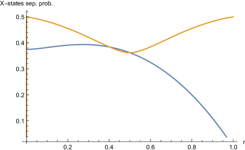
Figure 4: (Largely lower) $r_{A}=r_{B}$–given by (5)–and (largely upper) $r_{A}+r_{B}=1$ curves–given by (6)–for bivariate Hilbert-Schmidt $X$-states separability probability distribution. The minimum of the upper “antidiagonal” curve is at $r_{A}=\frac{1}{2}$, while the maximum of the lower “diagonal” curve is at 0.27227007. In the crossover interval $r_{A}\in[0.40182804,\frac{1}{2}]$, the $p^{(X)}_{HS}(r_{A},1-r_{A})$ curve is dominated by the $p^{(X)}_{HS}(r_{A},r_{A})$ curve.

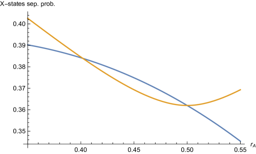
Figure 5: Closer examination of the $X$-states crossover region in Fig. 4, the lower bound being $\tilde{r}_{A}=0.40182804$, a root of the quintic equation (8)

References

- Jevtic et al. (2014) S. Jevtic, M. Pusey, D. Jennings, and T. Rudolph, Phys. Rev. Lett. 113, 020402 (2014).
- Milz and Strunz (2015) S. Milz and W. T. Strunz, J. Phys. A 48, 035306 (2015).
- Slater (2015) P. B. Slater, arXiv preprint arXiv:1506.08739 (2015).
- Gamel (2016) O. Gamel, Phys. Rev. A 93, 062320 (2016).
- Mendonça et al. (2014) P. Mendonça, M. A. Marchiolli, and D. Galetti, Ann. Phys. 351, 79 (2014).
- Slater (2007) P. B. Slater, J. Phys. A 40, 14279 (2007).
- Slater and Dunkl (2012) P. B. Slater and C. F. Dunkl, J. Phys. A 45, 095305 (2012).
- Slater (2013) P. B. Slater, J. Phys. A 46, 445302 (2013).
- (9) J. Fei and R. Joynt, eprint arXiv.1409:1993.
- Slater and Dunkl (2015a) P. B. Slater and C. F. Dunkl, J. Geom. Phys. 90, 42 (2015a).
- Khvedelidze and Rogojin (2015) A. Khvedelidze and I. Rogojin, Zap. Nauchn. Sem. POMI 432, 274 (2015).
- Fonseca-Romero et al. (2012) K. M. Fonseca-Romero, J. M. Martinez-Rincón, and C. Viviescas, Phys. Rev. A 86, 042325 (2012).
- Shang et al. (2015) J. Shang, Y.-L. Seah, H. K.Ng, D. J. Nott, and B.-T. Englert, New J. Phys. 17, 043017 (2015).
- Lovas and Andai (2016) A. Lovas and A. Andai, arXiv preprint arXiv:1610.01410 (2016).
- Slater and Dunkl (2015b) P. B. Slater and C. F. Dunkl, Adv. Math. Phys. 2015, 621353 (2015b).
- Życzkowski and Sommers (2001) K. Życzkowski and H.-J. Sommers, J. Phys. A A34, 7111 (2001).
- Aubrun et al. (2014) G. Aubrun, S. J. Szarek, and D. Ye, Commun. Pure Appl. Math. LXVII, 0129 (2014).
- Adachi et al. (2009) S. Adachi, M. Toda, and H. Kubotani, Annals of Physics 324, 2278 (2009).
- Braga et al. (2010) H. Braga, S. Souza, and S. S. Mizrahi, Phys. Rev. A 81, 042310 (2010).
- Sungur and Ng (2005) E. A. Sungur and P. Ng, Commun. Stat.–Theory and Methods 34, 2269 (2005).
- Ruschendorf et al. (1996) L. Ruschendorf, B. Schweizer, and M. D. Taylor, Distributions with fixed marginals and related topics (Institute of Mathematical Statistics, Hayward, CA, 1996).
- (22) J. I. de Vicente, Further results on entanglement detection and quantificiation from the correlation matrix criterion, eprint arXiv:0705.2583.
- Bengtsson and Życzkowski (2006) I. Bengtsson and K. Życzkowski, Geometry of Quantum States (Cambridge, Cambridge, 2006).
- Miszczak (2012) J. A. Miszczak, Comput. Phys. Commun. 183, 118 (2012).
- Miszczak (2013) J. A. Miszczak, Comput. Phys. Commun. 184, 257 (2013).
- Sommers and Życzkowski (2003) H.-J. Sommers and K. Życzkowski, J. Phys. A 36, 10083 (2003).
- Slater (2016) P. B. Slater, Quantum Information Processing pp. 1–16 (2016).
- Goyal et al. (2016) S. K. Goyal, B. N. Simon, R. Singh, and S. Simon, J. Phys. A 49, 165203 (2016).
- Szarek et al. (2006) S. Szarek, I. Bengtsson, and K. Życzkowski, J. Phys. A 39, L119 (2006).