Coresets for Scalable
Bayesian Logistic Regression

Abstract.

The use of Bayesian methods in large-scale data settings is attractive because of the rich hierarchical models, uncertainty quantification, and prior specification they provide. Standard Bayesian inference algorithms are computationally expensive, however, making their direct application to large datasets difficult or infeasible. Recent work on scaling Bayesian inference has focused on modifying the underlying algorithms to, for example, use only a random data subsample at each iteration. We leverage the insight that data is often redundant to instead obtain a weighted subset of the data (called a coreset) that is much smaller than the original dataset. We can then use this small coreset in any number of existing posterior inference algorithms without modification. In this paper, we develop an efficient coreset construction algorithm for Bayesian logistic regression models. We provide theoretical guarantees on the size and approximation quality of the coreset – both for fixed, known datasets, and in expectation for a wide class of data generative models. Crucially, the proposed approach also permits efficient construction of the coreset in both streaming and parallel settings, with minimal additional effort. We demonstrate the efficacy of our approach on a number of synthetic and real-world datasets, and find that, in practice, the size of the coreset is independent of the original dataset size. Furthermore, constructing the coreset takes a negligible amount of time compared to that required to run MCMC on it.

1. Introduction

Large-scale datasets, comprising tens or hundreds of millions of observations, are becoming the norm in scientific and commercial applications ranging from population genetics to advertising. At such scales even simple operations, such as examining each data point a small number of times, become burdensome; it is sometimes not possible to fit all data in the physical memory of a single machine. These constraints have, in the past, limited practitioners to relatively simple statistical modeling approaches. However, the rich hierarchical models, uncertainty quantification, and prior specification provided by Bayesian methods have motivated substantial recent effort in making Bayesian inference procedures, which are often computationally expensive, scale to the large-data setting.

The standard approach to Bayesian inference for large-scale data is to modify a specific inference algorithm, such as MCMC or variational Bayes, to handle distributed or streaming processing of data. Examples include subsampling and streaming methods for variational Bayes [22, 12, 13], subsampling methods for MCMC arxiv[37, 2, 7, 24, 27, 8]nips[37, 27, 8], and distributed “consensus” methods for MCMC [34, 35, 31, 14]. Existing methods, however, suffer from both practical and theoretical limitations. Stochastic variational inference [22] and subsampling MCMC methods use a new random subset of the data at each iteration, which requires random access to the data and hence is infeasible for very large datasets that do not fit into memory. Furthermore, in practice, subsampling MCMC methods have been found to require examining a constant fraction of the data at each iteration, severely limiting the computational gains obtained arxiv[30, 8, 36, 9, 3]nips[36, 9]. More scalable methods such as consensus MCMC arxiv[34, 35, 31, 14]nips[34, 35, 31] and streaming variational Bayes [12, 13] lead to gains in computational efficiency, but lack rigorous justification and provide no guarantees on the quality of inference.

An important insight in the large-scale setting is that much of the data is often redundant, though there may also be a small set of data points that are distinctive. For example, in a large document corpus, one news article about a hockey game may serve as an excellent representative of hundreds or thousands of other similar pieces about hockey games. However, there may only be a few articles about luge, so it is also important to include at least one article about luge. Similarly, one individual’s genetic information may serve as a strong representative of other individuals from the same ancestral population admixture, though some individuals may be genetic outliers. We leverage data redundancy to develop a scalable Bayesian inference framework that modifies the dataset instead of the common practice of modifying the inference algorithm. Our method, which can be thought of as a preprocessing step, constructs a coreset – a small, weighted subset of the data that approximates the full dataset [1, 15] – that can be used in many standard inference procedures to provide posterior approximations with guaranteed quality. The scalability of posterior inference with a coreset thus simply depends on the coreset’s growth with the full dataset size. To the best of our knowledge, coresets have not previously been used in a Bayesian setting.

The concept of coresets originated in computational geometry (e.g. [1]), but then became popular in theoretical computer science as a way to efficiently solve clustering problems such as $k$-means and PCA (see [15, 17] and references therein). Coreset research in the machine learning community has focused on scalable clustering in the optimization setting arxiv[17, 5, 26, 6]nips[26, 6], with the exception of Feldman et al. [16], who developed a coreset algorithm for Gaussian mixture models. Coreset-like ideas have previously been explored for maximum likelihood-learning of logistic regression models, though these methods either lack rigorous justification or have only asymptotic guarantees (see [21] and references thereinarxiv as well as [28], which develops a methodology applicable beyond logistic regression).

The job of the coreset in the Bayesian setting is to provide an approximation of the full data log-likelihood up to a multiplicative error uniformly over the parameter space. As this paper is the first foray into applying coresets in Bayesian inference, we begin with a theoretical analysis of the quality of the posterior distribution obtained from such an approximate log-likelihood. The remainder of the paper develops the efficient construction of small coresets for Bayesian logistic regression, a useful and widely-used model for the ubiquitous problem of binary classification. We develop a coreset construction algorithm, the output of which uniformly approximates the full data log-likelihood over parameter values in a ball with a user-specified radius. The approximation guarantee holds for a given dataset with high probability. We also obtain results showing that the boundedness of the parameter space is necessary for the construction of a nontrivial coreset, as well as results characterizing the algorithm’s expected performance under a wide class of data-generating distributions. Our proposed algorithm is applicable in both the streaming and distributed computation settings, and the coreset can then be used by any inference algorithm which accesses the (gradient of the) log-likelihood as a black box. Although our coreset algorithm is specifically for logistic regression, our approach is broadly applicable to other Bayesian generative models.

Experiments on a variety of synthetic and real-world datasets validate our approach and demonstrate robustness to the choice of algorithm hyperparameters. An empirical comparison to random subsampling shows that, in many cases, coreset-based posteriors are orders of magnitude better in terms of maximum mean discrepancy, including on a challenging 100-dimensional real-world dataset. Crucially, our coreset construction algorithm adds negligible computational overhead to the inference procedure. All proofs are deferred to the nipsAppendixarxivAppendix.

2. Problem Setting

We begin with the general problem of Bayesian posterior inference. Let $\mathcal{D}=\{(X_{n},Y_{n})\}_{n=1}^{N}$ be a dataset, where $X_{n}\in\mathcal{X}$ is a vector of covariates and $Y_{n}\in\mathcal{Y}$ is an observation. Let $\pi_{0}(\theta)$ be a prior density on a parameter $\theta\in\Theta$ and let $p(Y_{n}\,|\,X_{n},\theta)$ be the likelihood of observation $n$ given the parameter $\theta$. arxiv The Bayesian posterior is given by the density

$$\pi_{N}(\theta) :=\frac{\exp(\mathcal{L}_{N}(\theta))\pi_{0}(\theta)}{\mathcal{E}_{N}},$$ (2.1)

where $\mathcal{L}_{N}(\theta):=\sum_{n=1}^{N}\ln p(Y_{n}\,|\,X_{n},\theta)$ is the model log-likelihood and

$$\mathcal{E}_{N}:=\int\exp(\mathcal{L}_{N}(\theta))\pi_{0}(\theta)\,\mathrm{d}\theta$$ (2.2)

is the marginal likelihood (a.k.a. the model evidence). nips The Bayesian posterior is given by the density $\pi_{N}(\theta)$, where

$$\pi_{N}(\theta) :=\frac{\exp(\mathcal{L}_{N}(\theta))\pi_{0}(\theta)}{\mathcal{E}_{N}}, \mathcal{L}_{N}(\theta):=\sum_{n=1}^{N}\ln p(Y_{n}\,|\,X_{n},\theta), \mathcal{E}_{N}:=\int\exp(\mathcal{L}_{N}(\theta))\pi_{0}(\theta)\,\mathrm{d}\theta.$$ (2.3)

Our aim is to construct a weighted dataset $\tilde{\mathcal{D}}=\{(\gamma_{m},\tilde{X}_{m},\tilde{Y}_{m})\}_{m=1}^{M}$ with $M\ll N$ such that the weighted log-likelihood $\tilde{\mathcal{L}}_{N}(\theta)=\sum_{m=1}^{M}\gamma_{m}\ln p(\tilde{Y}_{n}\,|\,\tilde{X}_{m},\theta)$ satisfies

$$|\mathcal{L}_{N}(\theta)-\tilde{\mathcal{L}}_{N}(\theta)| \leq\varepsilon|\mathcal{L}_{N}(\theta)|,\quad\forall\theta\in\Theta.$$ (2.4)

If $\tilde{\mathcal{D}}$ satisfies Eq. 2.4, it is called an $\varepsilon$-coreset of $\mathcal{D}$, and the approximate posterior

$$\tilde{\pi}_{N}(\theta) =\frac{\exp(\tilde{\mathcal{L}}_{N}(\theta))\pi_{0}(\theta)}{\tilde{\mathcal{E}}_{N}}, \text{with}\quad\tilde{\mathcal{E}}_{N} =\int\exp(\tilde{\mathcal{L}}_{N}(\theta))\pi_{0}(\theta)\,\mathrm{d}\theta,$$ (2.5)

has a marginal likelihood $\tilde{\mathcal{E}}_{N}$ which approximates the true marginal likelihood $\mathcal{E}_{N}$, shown by Proposition 2.1. Thus, from a Bayesian perspective, the $\varepsilon$-coreset is a useful notion of approximation.

Proposition 2.1.

Let $\mathcal{L}(\theta)$ and $\tilde{\mathcal{L}}(\theta)$ be arbitrary non-positive log-likelihood functions that satisfy $|\mathcal{L}(\theta)-\tilde{\mathcal{L}}(\theta)|\leq\varepsilon|\mathcal{L}(\theta)|$ for all $\theta\in\Theta$. Then for any prior $\pi_{0}(\theta)$ such that the marginal likelihoods

$$\mathcal{E}=\int\exp(\mathcal{L}(\theta))\pi_{0}(\theta)\,\mathrm{d}\theta\qquad\text{and}\qquad\tilde{\mathcal{E}}=\int\exp(\tilde{\mathcal{L}}(\theta))\pi_{0}(\theta)\,\mathrm{d}\theta$$ (2.6)

are finite, the marginal likelihoods satisfy arxiv

$$|\ln\mathcal{E}-\ln\tilde{\mathcal{E}}|\leq\varepsilon|\ln\mathcal{E}|.$$ (2.7)

nips $|\ln\mathcal{E}-\ln\tilde{\mathcal{E}}|\leq\varepsilon|\ln\mathcal{E}|$.

3. Coresets for Logistic Regression

Algorithm 1 Construction of logistic regression coreset

1:Data $\mathcal{D}$, $k$-clustering $\mathcal{Q}$, radius $R>0$, tolerance $\varepsilon>0$, failure rate $\delta\in(0,1)$

2:for $n=1,\dots,N$ do $\triangleright$ calculate sensitivity upper bounds using the $k$-clustering

3:     $m_{n}\leftarrow\frac{N}{1+\sum_{i=1}^{k}|G_{i}^{(-n)}|e^{-R\|\bar{Z}_{G,i}^{(-n)}-Z_{n}\|_{2}}}$

4:end for

5:$\bar{m}_{N}\leftarrow\frac{1}{N}\sum_{n=1}^{N}m_{n}$

6:$M\leftarrow\left\lceil\frac{c\bar{m}_{N}}{\varepsilon^{2}}[(D+1)\log\bar{m}_{N}+\log(1/\delta)]\right\rceil$ $\triangleright$ coreset size; $c$ is from proof of Theorem B.1

7:for $n=1,\dots,N$ do

8:     $p_{n}\leftarrow\frac{m_{n}}{N\bar{m}_{N}}$ $\triangleright$ importance weights of data

9:end for

10:$(K_{1},\dots,K_{N})\sim{\sf{Multi}}(M,(p_{n})_{n=1}^{N})$ $\triangleright$ sample data for coreset

11:for $n=1,\dots,N$ do $\triangleright$ calculate coreset weights

12:     $\gamma_{n}\leftarrow\frac{K_{n}}{p_{n}M}$

13:end for

14:$\tilde{\mathcal{D}}\leftarrow\{(\gamma_{n},X_{n},Y_{n})\,|\,\gamma_{n}>0\}$ $\triangleright$ only keep data points with non-zero weights

15:return $\tilde{\mathcal{D}}$

3.1. Coreset Construction

In logistic regression, the covariates are real feature vectors $X_{n}\in\mathbb{R}^{D}$, the observations are labels $Y_{n}\in\{-1,1\}$, $\Theta\subseteq\mathbb{R}^{D}$, and the likelihood is defined as

$$p(Y_{n}\,|\,X_{n},\theta) =p_{logistic}(Y_{n}\,|\,X_{n},\theta):=\frac{1}{1+\exp\left(-Y_{n}X_{n}\cdot\theta\right)}.$$ (3.1)

The analysis in this work allows any prior $\pi_{0}(\theta)$; common choices are the Gaussian, Cauchy [18], and spike-and-slab arxiv[29, 19]nips[19]. For notational brevity, we define $Z_{n}:=Y_{n}X_{n}$, and let $\phi(s):=\ln(1+\exp(-s))$. Choosing the optimal $\epsilon$-coreset is not computationally feasible, so we take a less direct approach. We design our coreset construction algorithm and prove its correctness using a quantity $\sigma_{n}(\Theta)$ called the sensitivity [15], which quantifies the redundancy of a particular data point $n$ – the larger the sensitivity, the less redundant. In the setting of logistic regression, we have that the sensitivity is

$$\sigma_{n}(\Theta):=\sup_{\theta\in\Theta}\frac{N\,\phi(Z_{n}\cdot\theta)}{\sum_{\ell=1}^{N}\phi(Z_{\ell}\cdot\theta)}.$$ (3.2)

Intuitively, $\sigma_{n}(\Theta)$ captures how much influence data point $n$ has on the log-likelihood $\mathcal{L}_{N}(\theta)$ when varying the parameter $\theta\in\Theta$, and thus data points with high sensitivity should be included in the coreset. Evaluating $\sigma_{n}(\Theta)$ exactly is not tractable, however, so an upper bound $m_{n}\geq\sigma_{n}(\Theta)$ must be used in its place. Thus, the key challenge is to efficiently compute a tight upper bound on the sensitivity.

For the moment we will consider $\Theta=\mathbb{B}_{R}$ for any $R>0$, where $\mathbb{B}_{R}:=\{\theta\in\mathbb{R}^{D}\,|\,\|\theta\|_{2}\leq R\}$; we discuss the case of $\Theta=\mathbb{R}^{D}$ shortly. Choosing the parameter space to be a Euclidean ball is reasonable since data is usually preprocessed to have mean zero and variance 1 (or, for sparse data, to be between -1 and 1), so each component of $\theta$ is typically in a range close to zero (e.g. between -4 and 4) [18].

The idea behind our sensitivity upper bound construction is that we would expect data points that are bunched together to be redundant while data points that are far from from other data have a large effect on inferences. Clustering is an effective way to summarize data and detect outliers, so we will use a $k$-clustering of the data $\mathcal{D}$ to construct the sensitivity bound. A $k$-clustering is given by $k$ cluster centers $\mathcal{Q}=\{Q_{1},\dots,Q_{k}\}$. Let $G_{i}:=\{Z_{n}\,|\,i=\operatornamewithlimits{arg\,min}_{j}\|Q_{j}-Z_{n}\|_{2}\}$ be the set of vectors closest to center $Q_{i}$ and let $G_{i}^{(-n)}:=G_{i}\setminus\{Z_{n}\}$. Define $Z_{G,i}^{(-n)}$ to be a uniform random vector from $G_{i}^{(-n)}$ and let $\bar{Z}_{G,i}^{(-n)}:=\mathbb{E}[Z_{G,i}^{(-n)}]$ be its mean. The following lemma uses a $k$-clustering to establish an efficiently computable upper bound on $\sigma_{n}(\mathbb{B}_{R})$:

Lemma 3.1.

For any $k$-clustering $\mathcal{Q}$,

$$\sigma_{n}(\mathbb{B}_{R})\leq m_{n}:=\frac{N}{1+\sum_{i=1}^{k}|G_{i}^{(-n)}|e^{-R\|\bar{Z}_{G,i}^{(-n)}-Z_{n}\|_{2}}}.$$ (3.3)

Furthermore, $m_{n}$ can be calculated in $O(k)$ time.

The bound in Eq. 3.3 captures the intuition that if the data forms tight clusters (that is, each $Z_{n}$ is close to one of the cluster centers), we expect each cluster to be well-represented by a small number of typical data points. For example, if $Z_{n}\in G_{i}$, $\|\bar{Z}_{G,i}^{(-n)}-Z_{n}\|_{2}$ is small, and $|G_{i}^{(-n)}|=\Theta(N)$, then $\sigma_{n}(\mathbb{B}_{R})=O(1)$. We use the (normalized) sensitivity bounds obtained from Lemma 3.1 to form an importance distribution $(p_{n})_{n=1}^{N}$ from which to sample the coreset. If we sample $Z_{n}$, then we assign it weight $\gamma_{n}$ proportional to $1/p_{n}$. The size of the coreset depends on the mean sensitivity bound, the desired error $\varepsilon$, and a quantity closely related to the VC dimension of $\theta\mapsto\phi(\theta\cdot Z)$, which we show is $D+1$. Combining these pieces we obtain Algorithm 1, which constructs an $\varepsilon$-coreset with high probability by Theorem 3.2.

Theorem 3.2.

Fix $\varepsilon>0$, $\delta\in(0,1)$, and $R>0$. Consider a dataset $\mathcal{D}$ with $k$-clustering $\mathcal{Q}$. With probability at least $1-\delta$, Algorithm 1 with inputs $(\mathcal{D},\mathcal{Q},R,\varepsilon,\delta)$ constructs an $\varepsilon$-coreset of $\mathcal{D}$ for logistic regression with parameter space $\Theta=\mathbb{B}_{R}$. Furthermore, Algorithm 1 runs in $O(Nk)$ time.

Remark 3.3.

The coreset algorithm is efficient with an $O(Nk)$ running time. However, the algorithm requires a $k$-clustering, which must also be constructed. A high-quality clustering can be obtained cheaply via $k$-means++ in $O(Nk)$ time [4], although a coreset algorithm could also be used.

Examining Algorithm 1, we see that the coreset size $M$ is of order $\bar{m}_{N}\log\bar{m}_{N}$, where $\bar{m}_{N}=\frac{1}{N}\sum_{n}m_{n}$. So for $M$ to be smaller than $N$, at a minimum, $\bar{m}_{N}$ should satisfy $\bar{m}_{N}=\tilde{o}(N)$, and preferably $\bar{m}_{N}=O(1)$. Indeed, for the coreset size to be small, it is critical that (a) $\Theta$ is chosen such that most of the sensitivities satisfy $\sigma_{n}(\Theta)\ll N$ (since $N$ is the maximum possible sensitivity), (b) each upper bound $m_{n}$ is close to $\sigma_{n}(\Theta)$, and (c) ideally, that $\bar{m}_{N}$ is bounded by a constant. In Section 3.2, we address (a) by providing sensitivity lower bounds, thereby showing that the constraint $\Theta=\mathbb{B}_{R}$ is necessary for nontrivial sensitivities even for “typical” (i.e. non-pathological) data. We then apply our lower bounds to address (b) and show that our bound in Lemma 3.1 is nearly tight. In Section 3.3, we address (c) by establishing the expected performance of the bound in Lemma 3.1 for a wide class of data-generating distributions.

3.2. Sensitivity Lower Bounds

We now develop lower bounds on the sensitivity to demonstrate that essentially we must limit ourselves to bounded $\Theta$, thus making our choice of $\Theta=\mathbb{B}_{R}$ a natural one, and to show that the sensitivity upper bound from Lemma 3.1 is nearly tight.

We begin by showing that in both the worst case and the average case, for all $n$, $\sigma_{n}(\mathbb{R}^{D})=N$, the maximum possible sensitivity – even when the $Z_{n}$ are arbitrarily close. Intuitively, the reason for the worst-case behavior is that if there is a separating hyperplane between a data point $Z_{n}$ and the remaining data points, and $\theta$ is in the direction of that hyperplane, then when $\|\theta\|_{2}$ becomes very large, $Z_{n}$ becomes arbitrarily more important than any other data point.

Theorem 3.4.

For any $D\geq 3$, $N\in\mathbb{N}$ and $0<\epsilon^{\prime}<1$, there exists $\epsilon>0$ and unit vectors $Z_{1},\dots,Z_{N}\in\mathbb{R}^{D}$ such that for all pairs $n,n^{\prime}$, $Z_{n}\cdot Z_{n^{\prime}}\geq 1-\epsilon^{\prime}$ and for all $R>0$ and $n$,

$$\sigma_{n}(\mathbb{B}_{R}) \geq\frac{N}{1+(N-1)e^{-R\epsilon\mathchoice{{\hbox{$\displaystyle\sqrt{\epsilon^{\prime}\,}$}\lower 0.4pt\hbox{\vrule height=4.10278pt,depth=-3.28224pt}}}{{\hbox{$\textstyle\sqrt{\epsilon^{\prime}\,}$}\lower 0.4pt\hbox{\vrule height=4.10278pt,depth=-3.28224pt}}}{{\hbox{$\scriptstyle\sqrt{\epsilon^{\prime}\,}$}\lower 0.4pt\hbox{\vrule height=2.88748pt,depth=-2.31pt}}}{{\hbox{$\scriptscriptstyle\sqrt{\epsilon^{\prime}\,}$}\lower 0.4pt\hbox{\vrule height=2.28471pt,depth=-1.82779pt}}}/4}}, \sigma_{n}(\mathbb{R}^{D}) =N.$$ and hence (3.4)

The proof of Theorem 3.4 is based on choosing $N$ distinct unit vectors $V_{1},\dots,V_{N}\in\mathbb{R}^{D-1}$ and setting $\epsilon=1-\max_{n\neq n^{\prime}}V_{n}\cdot V_{n^{\prime}}>0$. But what is a “typical” value for $\epsilon$? In the case of the vectors being uniformly distributed on the unit sphere, we have the following scaling for $\epsilon$ as $N$ increases:

Proposition 3.5.

If $V_{1},\dots,V_{N}$ are independent and uniformly distributed on the unit sphere $\mathbb{S}^{D}:=\{v\in\mathbb{R}^{D}\,|\,\|v\|=1\}$ with $D\geq 2$, then with high probability

$$1-\max_{n\neq n^{\prime}}V_{n}\cdot V_{n^{\prime}}\geq C_{D}N^{-4/(D-1)},$$ (3.5)

where $C_{D}$ is a constant depending only on $D$.

Furthermore, $N$ can be exponential in $D$ even with $\epsilon$ remaining very close to 1:

Proposition 3.6.

For $N=\lfloor\exp((1-\epsilon)^{2}D/4)/\mathchoice{{\hbox{$\displaystyle\sqrt{2\,}$}\lower 0.4pt\hbox{\vrule height=6.44444pt,depth=-5.15558pt}}}{{\hbox{$\textstyle\sqrt{2\,}$}\lower 0.4pt\hbox{\vrule height=6.44444pt,depth=-5.15558pt}}}{{\hbox{$\scriptstyle\sqrt{2\,}$}\lower 0.4pt\hbox{\vrule height=4.51111pt,depth=-3.6089pt}}}{{\hbox{$\scriptscriptstyle\sqrt{2\,}$}\lower 0.4pt\hbox{\vrule height=3.22221pt,depth=-2.57779pt}}}\rfloor$, and $V_{1},\dots,V_{N}$ i.i.d. such that $V_{ni}=\pm\frac{1}{\mathchoice{{\hbox{$\displaystyle\sqrt{D\,}$}\lower 0.4pt\hbox{\vrule height=4.78333pt,depth=-3.82668pt}}}{{\hbox{$\textstyle\sqrt{D\,}$}\lower 0.4pt\hbox{\vrule height=4.78333pt,depth=-3.82668pt}}}{{\hbox{$\scriptstyle\sqrt{D\,}$}\lower 0.4pt\hbox{\vrule height=3.34833pt,depth=-2.67868pt}}}{{\hbox{$\scriptscriptstyle\sqrt{D\,}$}\lower 0.4pt\hbox{\vrule height=2.39166pt,depth=-1.91335pt}}}}$ with probability $\nicefrac{{1}}{{2}}$, then with probability at least $\nicefrac{{1}}{{2}}$, $1-\max_{n\neq n^{\prime}}V_{n}\cdot V_{n^{\prime}}\geq\epsilon.$

Propositions 3.5 and 3.6 demonstrate that the data vectors $Z_{n}$ found in Theorem 3.4 are, in two different senses, “typical” vectors and should not be thought of as worst-case data only occurring in some “negligible” or zero-measure set. These three results thus demonstrate that it is necessary to restrict attention to bounded $\Theta$. We can also use Theorem 3.4 to show that our sensitivity upper bound is nearly tight.

Corollary 3.7.

For the data $Z_{1},\dots,Z_{N}$ from Theorem 3.4,

$$\frac{N}{1+(N-1)e^{-R\epsilon\mathchoice{{\hbox{$\displaystyle\sqrt{\epsilon^{\prime}\,}$}\lower 0.4pt\hbox{\vrule height=4.10278pt,depth=-3.28224pt}}}{{\hbox{$\textstyle\sqrt{\epsilon^{\prime}\,}$}\lower 0.4pt\hbox{\vrule height=4.10278pt,depth=-3.28224pt}}}{{\hbox{$\scriptstyle\sqrt{\epsilon^{\prime}\,}$}\lower 0.4pt\hbox{\vrule height=2.88748pt,depth=-2.31pt}}}{{\hbox{$\scriptscriptstyle\sqrt{\epsilon^{\prime}\,}$}\lower 0.4pt\hbox{\vrule height=2.28471pt,depth=-1.82779pt}}}/4}}\leq\sigma_{n}(\mathbb{B}_{R})\leq\frac{N}{1+(N-1)e^{-R\mathchoice{{\hbox{$\displaystyle\sqrt{2\epsilon^{\prime}\,}$}\lower 0.4pt\hbox{\vrule height=4.51111pt,depth=-3.6089pt}}}{{\hbox{$\textstyle\sqrt{2\epsilon^{\prime}\,}$}\lower 0.4pt\hbox{\vrule height=4.51111pt,depth=-3.6089pt}}}{{\hbox{$\scriptstyle\sqrt{2\epsilon^{\prime}\,}$}\lower 0.4pt\hbox{\vrule height=3.15778pt,depth=-2.52625pt}}}{{\hbox{$\scriptscriptstyle\sqrt{2\epsilon^{\prime}\,}$}\lower 0.4pt\hbox{\vrule height=2.28471pt,depth=-1.82779pt}}}}}.$$ (3.6)

3.3. $k$-Clustering Sensitivity Bound Performance

While Lemmas 3.1 and 3.7 provide an upper bound on the sensitivity given a fixed dataset, we would also like to understand how the expected mean sensitivity increases with $N$. We might expect it to be finite since the logistic regression likelihood model is parametric; the coreset would thus be acting as a sort of approximate finite sufficient statistic. Proposition 3.8 characterizes the expected performance of the upper bound from Lemma 3.1 under a wide class of generating distributions. This result demonstrates that, under reasonable conditions, the expected value of $\bar{m}_{N}$ is bounded for all $N$. As a concrete example, Corollary 3.9 specializes Proposition 3.8 to data with a single shared Gaussian generating distribution.

Proposition 3.8.

Let $X_{n}\overset{\textrm{\tiny{indep}}}{\sim}\mathscr{N}(\mu_{L_{n}},\Sigma_{L_{n}})$, where $L_{n}\overset{\textrm{\tiny{indep}}}{\sim}{\sf{Multi}}(\pi_{1},\pi_{2},\dots)$ is the mixture component responsible for generating $X_{n}$. For $n=1,\dots,N$, let $Y_{n}\in\{-1,1\}$ be conditionally independent given $X_{n}$ and set $Z_{n}=Y_{n}X_{n}$. Select $0<r<1/2$, and define $\eta_{i}=\max(\pi_{i}-N^{-r},0)$. The clustering of the data implied by $(L_{n})_{n=1}^{N}$ results in the expected sensitivity bound

$$\mathbb{E}\left[\bar{m}_{N}\right] \leq\frac{1}{N^{-1}+\sum_{i}\eta_{i}e^{-R\mathchoice{{\hbox{$\displaystyle\sqrt{A_{i}N^{-1}\eta_{i}^{-1}+B_{i}\,}$}\lower 0.4pt\hbox{\vrule height=6.04643pt,depth=-4.83717pt}}}{{\hbox{$\textstyle\sqrt{A_{i}N^{-1}\eta_{i}^{-1}+B_{i}\,}$}\lower 0.4pt\hbox{\vrule height=6.04643pt,depth=-4.83717pt}}}{{\hbox{$\scriptstyle\sqrt{A_{i}N^{-1}\eta_{i}^{-1}+B_{i}\,}$}\lower 0.4pt\hbox{\vrule height=4.25055pt,depth=-3.40047pt}}}{{\hbox{$\scriptscriptstyle\sqrt{A_{i}N^{-1}\eta_{i}^{-1}+B_{i}\,}$}\lower 0.4pt\hbox{\vrule height=3.29388pt,depth=-2.63513pt}}}}}+\sum_{i:\eta_{i}>0}Ne^{-2N^{1-2r}}\overset{N\to\infty}{\to}\frac{1}{\sum_{i}\pi_{i}e^{-R\mathchoice{{\hbox{$\displaystyle\sqrt{B_{i}\,}$}\lower 0.4pt\hbox{\vrule height=4.78333pt,depth=-3.82668pt}}}{{\hbox{$\textstyle\sqrt{B_{i}\,}$}\lower 0.4pt\hbox{\vrule height=4.78333pt,depth=-3.82668pt}}}{{\hbox{$\scriptstyle\sqrt{B_{i}\,}$}\lower 0.4pt\hbox{\vrule height=3.34833pt,depth=-2.67868pt}}}{{\hbox{$\scriptscriptstyle\sqrt{B_{i}\,}$}\lower 0.4pt\hbox{\vrule height=2.39166pt,depth=-1.91335pt}}}}},$$ (3.7)

where arxiv

$$A_{i} :=\operatorname{Tr}\left[\Sigma_{i}\right]+\left(1-\bar{y}_{i}^{2}\right)\mu_{i}^{T}\mu_{i},$$ (3.8)

$$B_{i} :={\textstyle\sum_{j}}\pi_{j}\left(\operatorname{Tr}\left[\Sigma_{j}\right]+\bar{y}_{j}^{2}\mu_{i}^{T}\mu_{i}-2\bar{y}_{i}\bar{y}_{j}\mu_{i}^{T}\mu_{j}+\mu_{j}^{T}\mu_{j}\right),$$ (3.9)

and $\bar{y}_{j}=\mathbb{E}\left[Y_{1}|L_{1}=j\right]$. nips $A_{i}:=\operatorname{Tr}\left[\Sigma_{i}\right]+\left(1-\bar{y}_{i}^{2}\right)\mu_{i}^{T}\mu_{i}$, $B_{i}:={\textstyle\sum_{j}}\pi_{j}\left(\operatorname{Tr}\left[\Sigma_{j}\right]+\bar{y}_{j}^{2}\mu_{i}^{T}\mu_{i}-2\bar{y}_{i}\bar{y}_{j}\mu_{i}^{T}\mu_{j}+\mu_{j}^{T}\mu_{j}\right)$, and $\bar{y}_{j}=\mathbb{E}\left[Y_{1}|L_{1}=j\right]$.

Corollary 3.9.

In the setting of Proposition 3.8, if $\pi_{1}=1$ and all data is assigned to a single cluster, then there is a constant $C$ such that for sufficiently large $N$, nips $\mathbb{E}\left[\bar{m}_{N}\right]\leq Ce^{R\mathchoice{{\hbox{$\displaystyle\sqrt{\operatorname{Tr}\left[\Sigma_{1}\right]+(1-\bar{y}_{1}^{2})\mu_{1}^{T}\mu_{1}\,}$}\lower 0.4pt\hbox{\vrule height=6.94087pt,depth=-5.55272pt}}}{{\hbox{$\textstyle\sqrt{\operatorname{Tr}\left[\Sigma_{1}\right]+(1-\bar{y}_{1}^{2})\mu_{1}^{T}\mu_{1}\,}$}\lower 0.4pt\hbox{\vrule height=6.94087pt,depth=-5.55272pt}}}{{\hbox{$\scriptstyle\sqrt{\operatorname{Tr}\left[\Sigma_{1}\right]+(1-\bar{y}_{1}^{2})\mu_{1}^{T}\mu_{1}\,}$}\lower 0.4pt\hbox{\vrule height=6.57999pt,depth=-5.26402pt}}}{{\hbox{$\scriptscriptstyle\sqrt{\operatorname{Tr}\left[\Sigma_{1}\right]+(1-\bar{y}_{1}^{2})\mu_{1}^{T}\mu_{1}\,}$}\lower 0.4pt\hbox{\vrule height=6.57999pt,depth=-5.26402pt}}}}$. arxiv

$$\mathbb{E}\left[\bar{m}_{N}\right]\leq Ce^{R\mathchoice{{\hbox{$\displaystyle\sqrt{\operatorname{Tr}\left[\Sigma_{1}\right]+(1-\bar{y}_{1}^{2})\mu_{1}^{T}\mu_{1}\,}$}\lower 0.4pt\hbox{\vrule height=6.94087pt,depth=-5.55272pt}}}{{\hbox{$\textstyle\sqrt{\operatorname{Tr}\left[\Sigma_{1}\right]+(1-\bar{y}_{1}^{2})\mu_{1}^{T}\mu_{1}\,}$}\lower 0.4pt\hbox{\vrule height=6.94087pt,depth=-5.55272pt}}}{{\hbox{$\scriptstyle\sqrt{\operatorname{Tr}\left[\Sigma_{1}\right]+(1-\bar{y}_{1}^{2})\mu_{1}^{T}\mu_{1}\,}$}\lower 0.4pt\hbox{\vrule height=6.57999pt,depth=-5.26402pt}}}{{\hbox{$\scriptscriptstyle\sqrt{\operatorname{Tr}\left[\Sigma_{1}\right]+(1-\bar{y}_{1}^{2})\mu_{1}^{T}\mu_{1}\,}$}\lower 0.4pt\hbox{\vrule height=6.57999pt,depth=-5.26402pt}}}}.$$ (3.10)

3.4. Streaming and Parallel Settings

Algorithm 1 is a batch algorithm, but it can easily be used in parallel and streaming computation settings using standard methods from the coreset literature, which are based on the following two observations (cf. [16, Section 3.2]): nips

1. If $\tilde{\mathcal{D}}_{i}$ is an $\varepsilon$-coreset for $\mathcal{D}_{i}$, $i=1,2$, then $\tilde{\mathcal{D}}_{1}\cup\tilde{\mathcal{D}}_{2}$ is an $\varepsilon$-coreset for $\mathcal{D}_{1}\cup\mathcal{D}_{2}$.

2. If $\tilde{\mathcal{D}}$ is an $\varepsilon$-coreset for $\mathcal{D}$ and $\tilde{\mathcal{D}}^{\prime}$ is an $\varepsilon^{\prime}$-coreset for $\tilde{\mathcal{D}}$, then $\tilde{\mathcal{D}}^{\prime}$ is an $\varepsilon^{\prime\prime}$-coreset for $\mathcal{D}$, where $\varepsilon^{\prime\prime}:=(1+\varepsilon)(1+\varepsilon^{\prime})-1$.

nips We can use these observations to merge coresets that were constructed either in parallel, or sequentially, in a binary tree. Coresets are computed for two data blocks, merged using observation 1, then compressed further using observation 2. The next two data blocks have coresets computed and merged/compressed in the same manner, then the coresets from blocks 1&2 and 3&4 can be merged/compressed analogously. We continue in this way and organize the merge/compress operations into a binary tree. Then, if there are $B$ data blocks total, only $\log B$ blocks ever need be maintained simultaneously. In the streaming setting we would choose blocks of constant size, so $B=O(N)$, while in the parallel setting $B$ would be the number of machines available.

4. Experiments

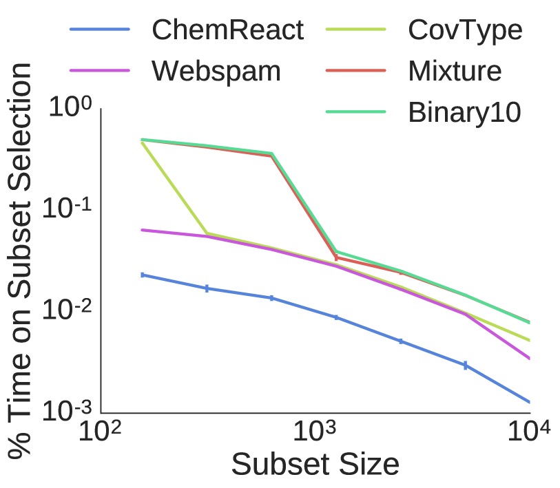
(a)

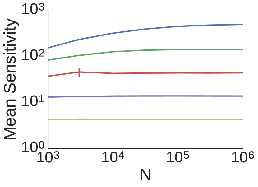
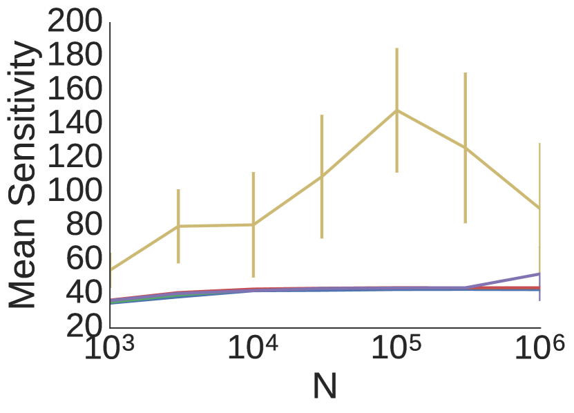
(b) Binary10

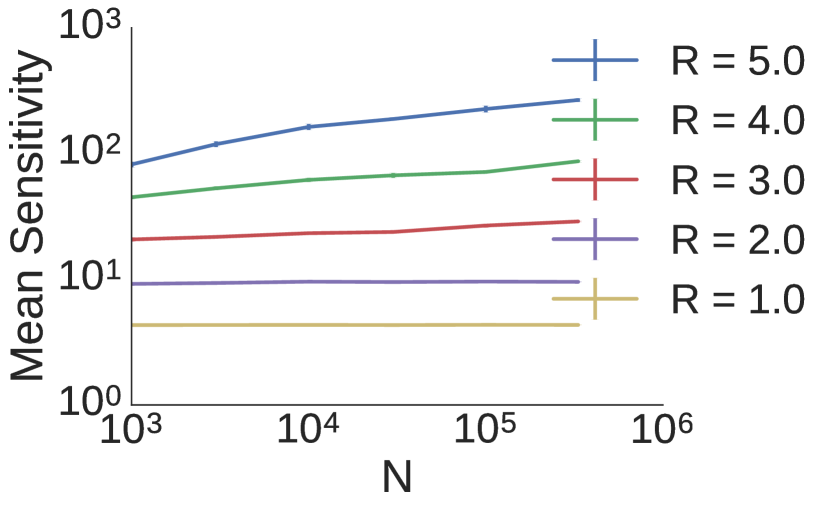
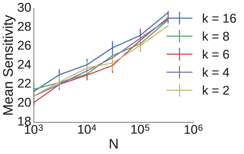
(c) Webspam

Figure 1. arxiv(A)nips(a) Percentage of time spent creating the coreset relative to the total inference time (including 10,000 iterations of MCMC). Except for very small coreset sizes, coreset construction is a small fraction of the overall time. arxiv(B,C)nips(b,c) The mean sensitivities for varying choices of $R$ and $k$. When $R$ varies $k=6$ and when $k$ varies $R=3$. The mean sensitivity increases exponentially in $R$, as expected, but is robust to the choice of $k$.

nips

arxiv nips

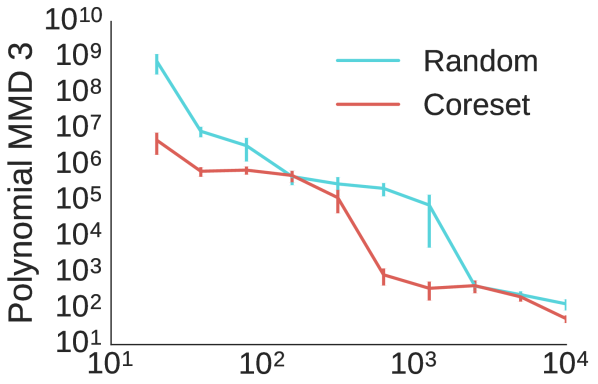
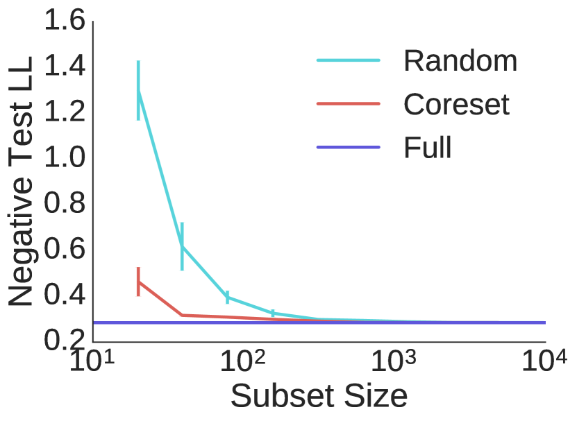
(a) Binary5

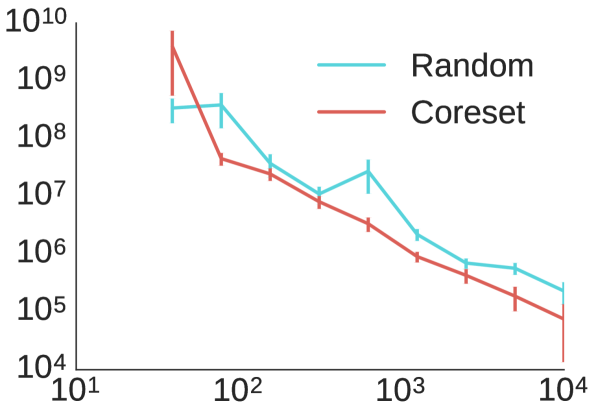
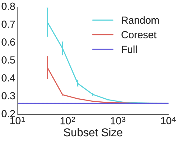
(b) Binary10

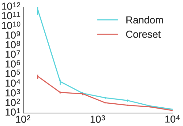
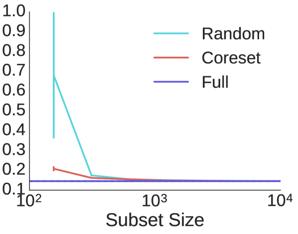
(c) Mixture

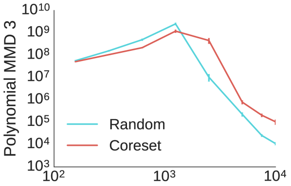
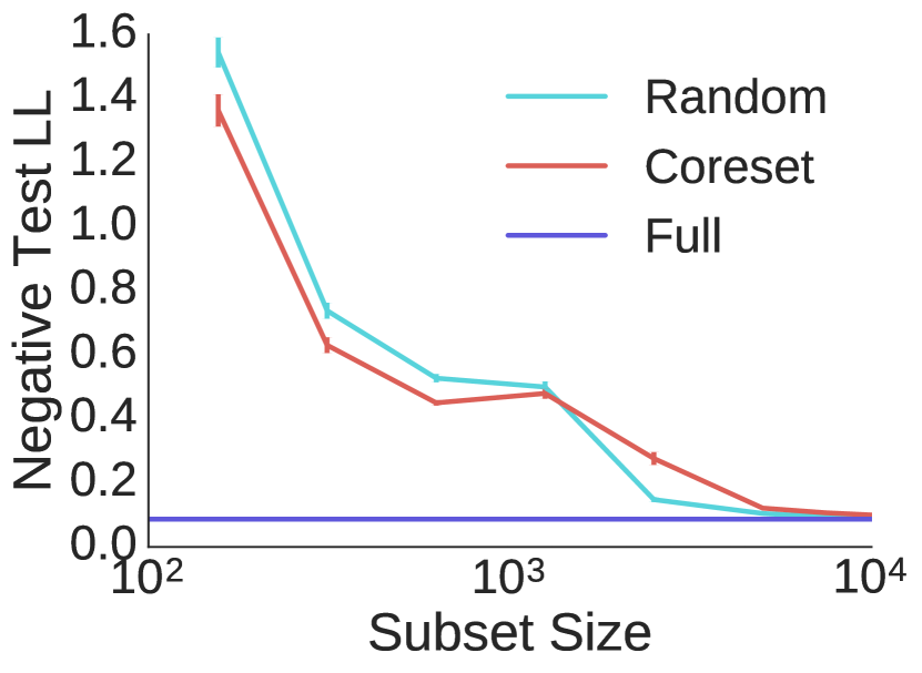
(d) ChemReact

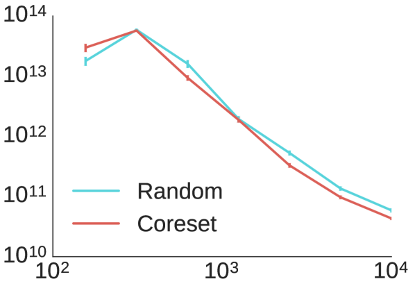
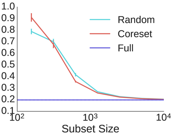
(e) Webspam

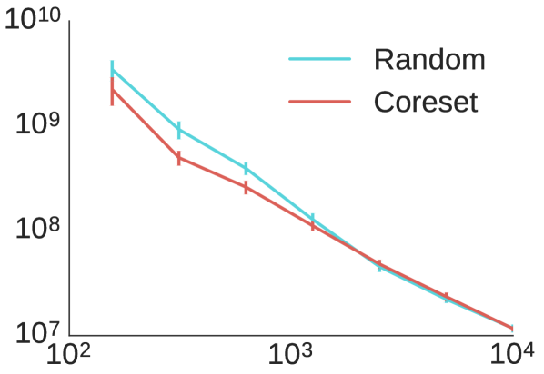
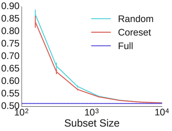
(f) CovType

Figure 2. Polynomial MMD and negative test log-likelihood of random sampling and the logistic regression coreset algorithm for synthetic and real data with varying subset sizes (lower is better for all plots). For the synthetic data, $N=10^{6}$ total data points were used and $10^{3}$ additional data points were generated for testing. For the real data, 2,500 (resp. 50,000 and 29,000) data points of the ChemReact (resp. Webspam and CovType) dataset were held out for testing. One standard deviation error bars were obtained by repeating each experiment 20 times.

nips

nips

We evaluated the performance of the logistic regression coreset algorithm on a number of synthetic and real-world datasets. We used a maximum dataset size of 1 million examples because we wanted to be able to calculate the true posterior, which would be infeasible for extremely large datasets.

Synthetic Data. We generated synthetic binary data according to the model $X_{nd}\overset{\textrm{\tiny{indep}}}{\sim}{\sf{Bern}}(p_{d}),d=1,\dots,D$ and $Y_{n}\overset{\textrm{\tiny{indep}}}{\sim}p_{logistic}(\cdot\,|\,X_{n},\theta)$. The idea is to simulate data in which there are a small number of rarely occurring but highly predictive features, which is a common real-world phenomenon. We thus took $p=(1,.2,.3,.5,.01,.1,.2,.007,.005,.001)$ and $\theta=(-3,1.2,-.5,.8,3,-1.,-.7,4,3.5,4.5)$ for the $D=10$ experiments (Binary10) and the first 5 components of $p$ and $\theta$ for the $D=5$ experiments (Binary5). The generative model is the same one used by Scott et al. [34] and the first 5 components of $p$ and $\theta$ correspond to those used in the Scott et al. experiments (given in [34, Table 1b]). We generated a synthetic mixture dataset with continuous covariates (Mixture) using a model similar to that of Han et al. [21]: $Y_{n}\overset{\textrm{\tiny{i.i.d.}}}{\sim}{\sf{Bern}}(1/2)$ and $X_{n}\overset{\textrm{\tiny{indep}}}{\sim}\mathscr{N}(\mu_{Y_{n}},I)$, where $\mu_{-1}=(0,0,0,0,0,1,1,1,1,1)$ and $\mu_{1}=(1,1,1,1,1,0,0,0,0,0)$.

Real-world Data. The ChemReact dataset consists of $N=$ 26,733 chemicals, each with $D=100$ properties. The goal is to predict whether each chemical is reactive. The Webspam corpus consists of $N=$ 350,000 web pages, approximately 60% of which are spam. The covariates consist of the $D=127$ features that each appear in at least 25 documents. The cover type (CovType) dataset consists of $N=$ 581,012 cartographic observations with $D=54$ features. The task is to predict the type of trees that are present at each observation location.

4.1. Scaling Properties of the Coreset Construction Algorithm

Constructing Coresets. In order for coresets to be a worthwhile preprocessing step, it is critical that the time required to construct the coreset is small relative to the time needed to complete the inference procedure. We implemented the logistic regression coreset algorithm in Python. In Fig. 1(a), we plot the relative time to construct the coreset for each type of dataset ($k=6$) versus the total inference time, including 10,000 iterations of the MCMC procedure described in Section 4.2. Except for very small coreset sizes, the time to run MCMC dominates.

Sensitivity. An important question is how the mean sensitivity $\bar{m}_{N}$ scales with $N$, as it determines how the size of the coreset scales with the data. Furthermore, ensuring that mean sensitivity is robust to the number of clusters $k$ is critical since needing to adjust the algorithm hyperparameters for each dataset could lead to an unacceptable increase in computational burden. We also seek to understand how the radius $R$ affects the mean sensitivity. Figs. 1(b) and 1(c) show the results of our scaling experiments on the Binary10 and Webspam data. The mean sensitivity is essentially constant across a range of dataset sizes. For both datasets the mean sensitivity is robust to the choice of $k$ and scales exponentially in $R$, as we would expect from Lemma 3.1. nips

4.2. Posterior Approximation Quality

Since the ultimate goal is to use coresets for Bayesian inference, the key empirical question is how well a posterior formed using a coreset approximates the true posterior distribution. We compared the coreset algorithm to random subsampling of data points, since that is the approach used in many existing scalable versions of variational inference and MCMC arxiv[22, 7, 24, 8]nips[22, 8]. Indeed, coreset-based importance sampling could be used as a drop-in replacement for the random subsampling used by these methods, though we leave the investigation of this idea for future work.

Experimental Setup. We used adaptive Metropolis-adjusted Langevin algorithm (MALA) [33, 20] for posterior inference. For each dataset, we ran the coreset and random subsampling algorithms 20 times for each choice of subsample size $M$. We ran adaptive MALA for 100,000 iterations on the full dataset and each subsampled dataset. The subsampled datasets were fixed for the entirety of each run, in contrast to subsampling algorithms that resample the data at each iteration. For the synthetic datasets, which are lower dimensional, we used $k=4$ while for the real-world datasets, which are higher dimensional, we used $k=6$. We used a heuristic to choose $R$ as large as was feasible while still obtaining moderate total sensitivity bounds. For a clustering $\mathcal{Q}$ of data $\mathcal{D}$, let $\mathcal{I}:=N^{-1}\sum_{i=1}^{k}\sum_{Z\in G_{i}}\|Z-Q_{i}\|^{2}$ be the normalized $k$-means score. We chose $R=a/\mathchoice{{\hbox{$\displaystyle\sqrt{\mathcal{I}\,}$}\lower 0.4pt\hbox{\vrule height=6.83331pt,depth=-5.46667pt}}}{{\hbox{$\textstyle\sqrt{\mathcal{I}\,}$}\lower 0.4pt\hbox{\vrule height=6.83331pt,depth=-5.46667pt}}}{{\hbox{$\scriptstyle\sqrt{\mathcal{I}\,}$}\lower 0.4pt\hbox{\vrule height=4.78333pt,depth=-3.82668pt}}}{{\hbox{$\scriptscriptstyle\sqrt{\mathcal{I}\,}$}\lower 0.4pt\hbox{\vrule height=3.41666pt,depth=-2.73334pt}}}$, where $a$ is a small constant. The idea is that, for $i\in[k]$ and $Z_{n}\in G_{i}$, we want $R\|\bar{Z}_{G,i}^{(-n)}-Z_{n}\|_{2}\approx a$ on average, so the term $\exp\{-R\|\bar{Z}_{G,i}^{(-n)}-Z_{n}\|_{2}\}$ in Eq. 3.3 is not too small and hence $\sigma_{n}(\mathbb{B}_{R})$ is not too large. Our experiments used $a=3$. We obtained similar results for $4\leq k\leq 8$ and $2.5\leq a\leq 3.5$, indicating that the logistic regression coreset algorithm has some robustness to the choice of these hyperparameters. We used negative test log-likelihood and maximum mean discrepancy (MMD) with a 3rd degree polynomial kernel as comparison metrics (so smaller is better).

Synthetic Data Results. Figures 2(a)-2(c) show the results for synthetic data. In terms of test log-likelihood, coresets did as well as or outperformed random subsampling. In terms of MMD, the coreset posterior approximation typically outperformed random subsampling by 1-2 orders of magnitude and never did worse. These results suggest much can be gained by using coresets, with comparable performance to random subsampling in the worst case.

Real-world Data Results. Figures 2(d)-2(f) show the results for real data. Using coresets led to better performance on ChemReact for small subset sizes. Because the dataset was fairly small and random subsampling was done without replacement, coresets were worse for larger subset sizes. Coreset and random subsampling performance was approximately the same for Webspam. On Webspam and CovType, coresets either outperformed or did as well as random subsampling in terms MMD and test log-likelihood on almost all subset sizes. The only exception was that random subsampling was superior on Webspam for the smallest subset set. We suspect this is due to the variance introduced by the importance sampling procedure used to generate the coreset.

For both the synthetic and real-world data, in many cases we are able to obtain a high-quality logistic regression posterior approximation using a coreset that is many orders of magnitude smaller than the full dataset – sometimes just a few hundred data points. Using such a small coreset represents a substantial reduction in the memory and computational requirements of the Bayesian inference algorithm that uses the coreset for posterior inference. We expect that the use of coresets could lead similar gains for other Bayesian models. Designing coreset algorithms for other widely-used models is an exciting direction for future research.

Acknowledgments

All authors are supported by the Office of Naval Research under ONR MURI grant N000141110688. JHH is supported by the U.S. Government under FA9550-11-C-0028 and awarded by the DoD, Air Force Office of Scientific Research, National Defense Science and Engineering Graduate (NDSEG) Fellowship, 32 CFR 168a.

Appendix A Marginal Likelihood Approximation

Proof of Proposition 2.1.

By the assumption that $\mathcal{L}$ and $\tilde{\mathcal{L}}$ are non-positive, the multiplicative error assumption, and Jensen’s inequality,

$$\tilde{\mathcal{E}} =\int e^{\tilde{\mathcal{L}}(\theta)}\pi_{0}(\theta)\,\mathrm{d}\theta\geq\int e^{(1+\varepsilon)\mathcal{L}(\theta)}\pi_{0}(\theta)\,\mathrm{d}\theta\geq\left(\int e^{\mathcal{L}(\theta)}\pi_{0}(\theta)\,\mathrm{d}\theta\right)^{1+\varepsilon}=\mathcal{E}^{1+\varepsilon}$$ (A.1)

and

$$\tilde{\mathcal{E}} =\int e^{\tilde{\mathcal{L}}(\theta)}\pi_{0}(\theta)\,\mathrm{d}\theta\leq\int e^{(1-\varepsilon)\mathcal{L}(\theta)}\pi_{0}(\theta)\,\mathrm{d}\theta\leq\left(\int e^{\mathcal{L}(\theta)}\pi_{0}(\theta)\,\mathrm{d}\theta\right)^{1-\varepsilon}=\mathcal{E}^{1-\varepsilon}.$$ (A.2)

∎

Appendix B Main Results

In order to construct coresets for logistic regression, we will use the framework developed by Feldman and Langberg [15] and improved upon by Braverman et al. [11]. For $n\in[N]:=\{1,\dots,N\}$, let $f_{n}:\mathcal{S}\to\mathbb{R}_{+}$ be a non-negative function from some set $\mathcal{S}$ and let $\bar{f}=\frac{1}{N}\sum_{n=1}^{N}f_{n}$ be the average of the functions. Define the sensitivity of $n\in[N]$ with respect to $\mathcal{S}$ by

$$\sigma_{n}(\mathcal{S}):=\sup_{s\in S}\frac{f_{n}(s)}{\bar{f}(s)},$$ (B.1)

and note that $\sigma_{n}(\mathcal{S})\leq N$. Also, for the set $\mathcal{F}:=\{f_{n}\,|\,n\in[N]\}$, define the dimension $\dim(\mathcal{F})$ of $\mathcal{F}$ to be the minimum integer $d$ such that

$$\forall F\subseteq\mathcal{F},\;|\{F\cap R\,|\,R\in\textbf{ranges}(\mathcal{F})\}|\leq(|F|+1)^{d},$$ (B.2)

where $\textbf{ranges}(\mathcal{F}):=\{\textbf{range}(s,a)|s\in\mathcal{S},a\geq 0\}$ and $\textbf{range}(s,a):=\{f\in\mathcal{F}\,|\,f(s)\leq a\}$.

We make use of the following improved version of Feldman and Langberg [15, Theorems 4.1 and 4.4].

Theorem B.1 (Braverman et al. [11]).

Fix $\varepsilon>0$. For $n\in[N]$, let $m_{n}\in\mathbb{R}_{+}$ be chosen such that

$$m_{n}\geq\sigma_{n}(\mathcal{S})$$ (B.3)

and let $\bar{m}_{N}:=\frac{1}{N}\sum_{n=1}^{N}m_{n}$. There is a universal constant $c$ such that if $\mathcal{C}$ is a sample from $\mathcal{F}$ of size

$$|\mathcal{C}|\geq\frac{c\,\bar{m}_{N}}{\varepsilon^{2}}(\dim(\mathcal{F})\log\bar{m}_{N}+\ln(1/\delta)),$$ (B.4)

such that the probability that each element of $\mathcal{C}$ is selected independently from $\mathcal{F}$ with probability $\frac{m_{n}}{N\bar{m}_{N}}$ that $f_{n}$ is chosen, then with probability at least $1-\delta$, for all $s\in\mathcal{S}$,

$$\left|\bar{f}(s)-\frac{\bar{m}_{N}}{|\mathcal{C}|}{\textstyle\sum_{f\in\mathcal{C}}}\frac{f(s)}{m_{n}}\right|\leq\varepsilon\bar{f}(s).$$ (B.5)

The set $\mathcal{C}$ in the theorem is called a coreset. In our application to logistic regression, $\mathcal{S}=\Theta$ and $f_{n}(\theta)=-\ln p(Y_{n}\,|\,X_{n},\theta)$. The key is to determine $\dim(\mathcal{F})$ and to construct the values $m_{n}$ efficiently. Furthermore, it is necessary for $\bar{m}_{N}=o(\mathchoice{{\hbox{$\displaystyle\sqrt{N\,}$}\lower 0.4pt\hbox{\vrule height=6.83331pt,depth=-5.46667pt}}}{{\hbox{$\textstyle\sqrt{N\,}$}\lower 0.4pt\hbox{\vrule height=6.83331pt,depth=-5.46667pt}}}{{\hbox{$\scriptstyle\sqrt{N\,}$}\lower 0.4pt\hbox{\vrule height=4.78333pt,depth=-3.82668pt}}}{{\hbox{$\scriptscriptstyle\sqrt{N\,}$}\lower 0.4pt\hbox{\vrule height=3.41666pt,depth=-2.73334pt}}})$ at a minimum and preferable for $\bar{m}_{N}=O(1)$.

Letting $Z_{n}=Y_{n}X_{n}$ and $\phi(s)=\ln(1+\exp(-s))$, we can rewrite $f_{n}(\theta)=\phi(Z_{n}\cdot\theta)$. Hence, the goal is to find an upper bound

$$m_{n}\geq\sigma_{n}(\Theta)=\sup_{\theta\in\Theta}\frac{N\,\phi(Z_{n}\cdot\theta)}{\sum_{n^{\prime}=1}^{N}\phi(Z_{n^{\prime}}\cdot\theta)}.$$ (B.6)

To obtain an upper bound on the sensitivity, we will take $\Theta=\mathbb{B}_{R}$ for some $R>0$.

Lemma B.2.

For all $a,b\in\mathbb{R}$, $\phi(a)/\phi(b)\leq e^{|a-b|}$.

Proof.

The lemma is trivial when $a=b$. Let $\Delta=b-a\neq 0$ and $\rho(a)=\phi(a)/\phi(a+\Delta)$. We have

$$\rho^{\prime}(a)=\frac{(1+e^{a})\log(1+e^{-a})-(1+e^{a+\Delta})\log(1+e^{-a-\Delta})}{(1+e^{a})(1+e^{a+\Delta})\log^{2}(1+e^{-a-\Delta})}.$$ (B.7)

Examining the previous display we see that $\operatorname{sgn}(\rho^{\prime}(a))=\operatorname{sgn}(\Delta)$. Hence if $\Delta>0$,

$$\sup_{a}\frac{\phi(a)}{\phi(a+\Delta)} =\lim_{a\to\infty}\frac{\phi(a)}{\phi(a+\Delta)}$$ (B.8)

$$=\lim_{a\to\infty}\frac{\phi^{\prime}(a)}{\phi^{\prime}(a+\Delta)}$$ (B.9)

$$=\lim_{a\to\infty}\frac{e^{-a}}{1+e^{-a}}\frac{1+e^{-a-\Delta}}{e^{-a-\Delta}}$$ (B.10)

$$=e^{\Delta}=e^{|b-a|},$$ (B.11)

where the second equality follows from L’Hospital’s rule. Similarly, if $\Delta<0$,

$$\sup_{a}\frac{\phi(a)}{\phi(a+\Delta)} =\lim_{a\to-\infty}\frac{e^{-a}}{1+e^{-a}}\frac{1+e^{-a-\Delta}}{e^{-a-\Delta}}$$ (B.12)

$$=\lim_{a\to-\infty}e^{\Delta}\frac{e^{-a}}{e^{-a-\Delta}}$$ (B.13)

$$=1\leq e^{|b-a|},$$ (B.14)

where in this case we have used L’Hospital’s rule twice. ∎

Lemma B.3.

The function $\phi(s)$ is convex.

Proof.

A straightforward calculation shows that $\phi^{\prime\prime}(s)=\frac{e^{s}}{(1+e^{s})^{2}}>0$. ∎

Lemma B.4.

For a random vector $Z\in\mathbb{R}^{D}$ with finite mean $\bar{Z}=\mathbb{E}[Z]$ and a fixed vectors $V,\theta^{*}\in\mathbb{R}^{D}$,

$$\inf_{\theta\in\mathbb{B}_{R}}\mathbb{E}\left[\frac{\phi(Z\cdot(\theta+\theta^{*}))}{\phi(V\cdot(\theta+\theta^{*}))}\right]\geq e^{-R\|\bar{Z}-V\|_{2}-|(\bar{Z}-V)\cdot\theta^{*}|}.$$ (B.15)

Proof.

Using Lemmas B.2 and B.3, Jensen’s inequality, and the triangle inequality, we have

$$\inf_{\theta\in\mathbb{B}_{R}}\mathbb{E}\left[\frac{\phi(Z\cdot(\theta+\theta^{*}))}{\phi(V\cdot(\theta+\theta^{*}))}\right] \geq\inf_{\theta\in\mathbb{B}_{R}}\frac{\phi(\mathbb{E}[Z]\cdot(\theta+\theta^{*}))}{\phi(V\cdot(\theta+\theta^{*}))}$$ (B.16)

$$\geq\inf_{\theta\in\mathbb{B}_{R}}e^{-|(\bar{Z}-V)\cdot(\theta+\theta^{*})|}$$ (B.17)

$$\geq\inf_{\theta\in\mathbb{B}_{R}}e^{-|(\bar{Z}-V)\cdot\theta|-|(\bar{Z}-V)\cdot\theta^{*})|}$$ (B.18)

$$=e^{-R\|\bar{Z}-V\|_{2}-|(\bar{Z}-V)\cdot\theta^{*}|}.$$ (B.19)

∎

We now prove the following generalization of Lemma 3.1

Lemma B.5.

For any $k$-clustering $\mathcal{Q}$, $\theta^{*}\in\mathbb{R}^{d}$, and $R>0$,

$$\sigma_{n}(\theta^{*}+\mathbb{B}_{R})\leq m_{n}:=\left\lceil\frac{N}{1+\sum_{i=1}^{k}|G_{i}^{(-n)}|e^{-R\|\bar{Z}_{G,i}^{(-n)}-Z_{n}\|_{2}-|(\bar{Z}_{G,i}^{(-n)}-Z_{n})\cdot\theta^{*}|}}\right\rceil.$$ (B.20)

Furthermore, $m_{n}$ can be calculated in $O(k)$ time.

Proof.

Straightforward manipulations followed by an application of Lemma B.4 yield

$$\sigma_{n}(\theta^{*}+\mathbb{B}_{R})^{-1} =\inf_{\theta\in\mathbb{B}_{R}}\frac{1}{N}\sum_{n^{\prime}=1}^{N}\frac{\phi(Z_{n^{\prime}}\cdot(\theta+\theta^{*}))}{\phi(Z_{n}\cdot(\theta+\theta^{*}))}$$ (B.21)

$$=\inf_{\theta\in\mathbb{B}_{R}}\frac{1}{N}\left[1+\sum_{i=1}^{k}\sum_{Z^{\prime}\in G_{i}^{(-n)}}\frac{\phi(Z^{\prime}\cdot(\theta+\theta^{*}))}{\phi(Z_{n}\cdot(\theta+\theta^{*}))}\right]$$ (B.22)

$$=\inf_{\theta\in\mathbb{B}_{R}}\frac{1}{N}\left[1+\sum_{i=1}^{k}|G_{i}^{(-n)}|\,\mathbb{E}\left[\frac{\phi(Z_{G,i}^{(-n)}\cdot(\theta+\theta^{*}))}{\phi(Z_{n}\cdot(\theta+\theta^{*}))}\right]\right]$$ (B.23)

$$\geq\frac{1}{N}\left[1+\sum_{i=1}^{k}|G_{i}^{(-n)}|e^{-R\|\bar{Z}_{G,i}^{(-n)}-Z_{n}\|_{2}-|(\bar{Z}_{G,i}^{(-n)}-Z_{n})\cdot\theta^{*}|}\right].$$ (B.24)

To see that the bound can be calculated in $O(k)$ time, first note that the cluster $i_{n}$ to which $Z_{n}$ belongs can be found in $O(k)$ time while $\bar{Z}_{G,i_{n}}^{(-n)}$ can be calculated in $O(1)$ time. For $i\neq i_{n}$, $G_{i}^{(-n)}=G_{i}$, so $\bar{Z}_{G,i}^{(-n)}$ is just the mean of cluster $i$, and no extra computation is required. Finally, computing the sum takes $O(k)$ time. ∎

In order to obtain an algorithm for generating coresets for logistic regression, we require a bound on the dimension of the range space constructed from the examples and logistic regression likelihood.

Proposition B.6.

The set of functions $\mathcal{F}=\{f_{n}(\theta)=\phi(Z_{n}\cdot\theta)\,|\,n\in[N]\}$ satisfies $\dim(\mathcal{F})\leq D+1$.

Proof.

For all $F\subseteq\mathcal{F}$,

$$|\{F\cap R\,|\,R\in\textbf{ranges}(\mathcal{F})\}| =|\{\textbf{range}(F,\theta,a)\,|\,\theta\in\Theta,a\geq 0\}|,$$ (B.25)

where $\textbf{range}(F,\theta,a):=\{f_{n}\in\mathcal{F}\,|\,f_{n}(\theta)\leq a\}$. But, since $\phi$ is invertible and monotonic,

$$\{f_{n}\in\mathcal{F}\,|\,f_{n}(\theta)\leq a\} =\{f_{n}\in\mathcal{F}\,|\,\phi(Z_{n}\cdot\theta)\leq a\}$$ (B.26)

$$=\{f_{n}\in\mathcal{F}\,|\,Z_{n}\cdot\theta\leq\phi^{-1}(a)\},$$ (B.27)

which is exactly a set of points shattered by the hyperplane classifier $Z\mapsto\operatorname{sgn}(Z\cdot\theta-b)$, with $b:=\phi^{-1}(a)$. Since the VC dimension of the hyperplane concept class is $D+1$, it follows that [23, Lemmas 3.1 and 3.2]

$$|\{\textbf{range}(F,\theta,a)\,|\,\theta\in\Theta,a\geq 0\}| \leq\sum_{j=0}^{D+1}{|F|\choose j}\leq\sum_{j=0}^{D+1}\frac{|F|^{j}}{j!}$$ (B.28)

$$\leq\sum_{j=0}^{D+1}{D+1\choose j}|F|^{j}=(|F|+1)^{D+1}.$$ (B.29)

∎

Proof of Theorem 3.2.

Combine Theorems B.1, 3.1 and B.6. The algorithm has overall complexity $O(Nk)$ since it requires $O(Nk)$ time to calculate the sensitivities by Lemma 3.1 and $O(N)$ time to sample the coreset. ∎

Appendix C Sensitivity Lower Bounds

Lemma C.1.

Let $V_{1},\dots,V_{K}\in\mathbb{R}^{D-1}$ be unit vectors such that for some $\epsilon>0$, for all $k\neq k$’, $V_{k}\cdot V_{k^{\prime}}\leq 1-\epsilon$. Then for $0<\delta<\mathchoice{{\hbox{$\displaystyle\sqrt{1/2\,}$}\lower 0.4pt\hbox{\vrule height=7.5pt,depth=-6.00003pt}}}{{\hbox{$\textstyle\sqrt{1/2\,}$}\lower 0.4pt\hbox{\vrule height=7.5pt,depth=-6.00003pt}}}{{\hbox{$\scriptstyle\sqrt{1/2\,}$}\lower 0.4pt\hbox{\vrule height=5.25pt,depth=-4.20003pt}}}{{\hbox{$\scriptscriptstyle\sqrt{1/2\,}$}\lower 0.4pt\hbox{\vrule height=3.75pt,depth=-3.00002pt}}}$, there exist unit vectors $Z_{1},\dots,Z_{K}\in\mathbb{R}^{D}$ such that

• for $k\neq k^{\prime}$, $Z_{k}\cdot Z_{k^{\prime}}\geq 1-2\delta^{2}>0$

• for $k=1,\dots,K$ and $\alpha>0$, there exists $\theta_{k}\in\mathbb{R}^{D}$ such that $\|\theta\|_{2}\leq\mathchoice{{\hbox{$\displaystyle\sqrt{2\,}$}\lower 0.4pt\hbox{\vrule height=6.44444pt,depth=-5.15558pt}}}{{\hbox{$\textstyle\sqrt{2\,}$}\lower 0.4pt\hbox{\vrule height=6.44444pt,depth=-5.15558pt}}}{{\hbox{$\scriptstyle\sqrt{2\,}$}\lower 0.4pt\hbox{\vrule height=4.51111pt,depth=-3.6089pt}}}{{\hbox{$\scriptscriptstyle\sqrt{2\,}$}\lower 0.4pt\hbox{\vrule height=3.22221pt,depth=-2.57779pt}}}\delta\alpha$, $\theta_{k}\cdot Z_{k}=-\frac{\alpha\epsilon\delta^{2}}{2}$ and for $k\neq k$, $\theta_{k}\cdot Z_{k^{\prime}}\geq\frac{\alpha\epsilon\delta^{2}}{2}$.

Proof.

Let $Z_{k}$ be defined such that $Z_{ki}=\delta V_{ki}$ for $i=1,\dots,D-1$ and $Z_{kD}=\mathchoice{{\hbox{$\displaystyle\sqrt{1-\delta^{2}\,}$}\lower 0.4pt\hbox{\vrule height=8.74889pt,depth=-6.99915pt}}}{{\hbox{$\textstyle\sqrt{1-\delta^{2}\,}$}\lower 0.4pt\hbox{\vrule height=8.74889pt,depth=-6.99915pt}}}{{\hbox{$\scriptstyle\sqrt{1-\delta^{2}\,}$}\lower 0.4pt\hbox{\vrule height=6.14998pt,depth=-4.92001pt}}}{{\hbox{$\scriptscriptstyle\sqrt{1-\delta^{2}\,}$}\lower 0.4pt\hbox{\vrule height=4.7611pt,depth=-3.8089pt}}}$. Thus, $\|Z_{k}\|_{2}=1$ and for $k\neq k^{\prime}$,

$$Z_{k}\cdot Z_{k^{\prime}}=\delta^{2}V_{k}\cdot V_{k^{\prime}}+1-\delta^{2}\geq 1-2\delta^{2}$$ (C.1)

since $V_{k}\cdot V_{k^{\prime}}\geq-1$. Let $\theta_{k}$ be such that $\theta_{ki}=-\alpha\delta V_{ki}$ for $i=1,\dots,D-1$ and $\theta_{kd}=\frac{\alpha\delta^{2}(1-\epsilon/2)}{\mathchoice{{\hbox{$\displaystyle\sqrt{1-\delta^{2}\,}$}\lower 0.4pt\hbox{\vrule height=6.1242pt,depth=-4.8994pt}}}{{\hbox{$\textstyle\sqrt{1-\delta^{2}\,}$}\lower 0.4pt\hbox{\vrule height=6.1242pt,depth=-4.8994pt}}}{{\hbox{$\scriptstyle\sqrt{1-\delta^{2}\,}$}\lower 0.4pt\hbox{\vrule height=4.305pt,depth=-3.44402pt}}}{{\hbox{$\scriptscriptstyle\sqrt{1-\delta^{2}\,}$}\lower 0.4pt\hbox{\vrule height=3.33276pt,depth=-2.66623pt}}}}$. Hence,

$$\theta_{k}\cdot\theta_{k} =\alpha^{2}\delta^{2}\left(V_{k}\cdot V_{k}+\frac{(1-\epsilon/2)^{2}\delta^{2}}{1-\delta^{2}}\right)\leq 2\alpha^{2}\delta^{2}$$ (C.2)

$$\theta_{k}\cdot Z_{k} =\alpha(-\delta^{2}V_{k}\cdot V_{k}+\delta^{2}(1-\epsilon/2))=-\frac{\alpha\epsilon\delta^{2}}{2},$$ (C.3)

and for $k^{\prime}\neq k$,

$$\theta_{k}\cdot Z_{k^{\prime}}=\alpha(-\delta^{2}V_{k}\cdot V_{k^{\prime}}+\delta^{2}(1-\epsilon/2))\geq\alpha\delta^{2}(-1+\epsilon+1-\epsilon/2)=\frac{\alpha\epsilon\delta^{2}}{2}.$$ (C.4)

∎

Proposition C.2.

Let $V_{1},\dots,V_{K}\in\mathbb{R}^{D-1}$ be unit vectors such that for some $\epsilon>0$, for all $k\neq k$’, $V_{k}\cdot V_{k^{\prime}}\leq 1-\epsilon$. Then for any $0<\epsilon^{\prime}<1$, there exist unit vectors $Z_{1},\dots,Z_{K}\in\mathbb{R}^{D}$ such that for $k,k^{\prime}$, $Z_{k}\cdot Z_{k^{\prime}}\geq 1-\epsilon^{\prime}$ but for any $R>0$,

$$\sigma_{k}(\mathbb{B}_{R})\geq\frac{K}{1+(K-1)e^{-R\epsilon\mathchoice{{\hbox{$\displaystyle\sqrt{\epsilon^{\prime}\,}$}\lower 0.4pt\hbox{\vrule height=4.10278pt,depth=-3.28224pt}}}{{\hbox{$\textstyle\sqrt{\epsilon^{\prime}\,}$}\lower 0.4pt\hbox{\vrule height=4.10278pt,depth=-3.28224pt}}}{{\hbox{$\scriptstyle\sqrt{\epsilon^{\prime}\,}$}\lower 0.4pt\hbox{\vrule height=2.88748pt,depth=-2.31pt}}}{{\hbox{$\scriptscriptstyle\sqrt{\epsilon^{\prime}\,}$}\lower 0.4pt\hbox{\vrule height=2.28471pt,depth=-1.82779pt}}}/4}},$$ (C.5)

and hence $\sigma_{k}(\mathbb{R}^{D})=K$.

Proof.

Let $Z_{1},\dots,Z_{K}\in\mathbb{R}^{D}$ be as in Lemma C.1 with $\delta$ such that $\delta^{2}=\epsilon^{\prime}/2$. Since for $s\geq 0$, $\phi(s)/\phi(-s)\leq e^{-s}$, conclude that, choosing $\alpha$ such that $\mathchoice{{\hbox{$\displaystyle\sqrt{2\,}$}\lower 0.4pt\hbox{\vrule height=6.44444pt,depth=-5.15558pt}}}{{\hbox{$\textstyle\sqrt{2\,}$}\lower 0.4pt\hbox{\vrule height=6.44444pt,depth=-5.15558pt}}}{{\hbox{$\scriptstyle\sqrt{2\,}$}\lower 0.4pt\hbox{\vrule height=4.51111pt,depth=-3.6089pt}}}{{\hbox{$\scriptscriptstyle\sqrt{2\,}$}\lower 0.4pt\hbox{\vrule height=3.22221pt,depth=-2.57779pt}}}\alpha\delta=R$, we have

$$\sigma_{n}(\mathbb{B}_{R}) =\sup_{\theta\in\mathbb{B}_{R}}\frac{K\,\phi(Z_{k}\cdot\theta)}{\sum_{k^{\prime}=1}^{K}\phi(Z_{k^{\prime}}\cdot\theta)}$$ (C.6)

$$\geq\frac{K\,\phi(-\alpha\epsilon\delta^{2}/2)}{\phi(-\alpha\epsilon\delta^{2}/2)+(K-1)\phi(\alpha\epsilon\delta^{2}/2)}$$ (C.7)

$$\geq\frac{K}{1+(K-1)e^{-\alpha\epsilon\delta^{2}/2}}$$ (C.8)

$$=\frac{K}{1+(K-1)e^{-R\epsilon\mathchoice{{\hbox{$\displaystyle\sqrt{\epsilon^{\prime}\,}$}\lower 0.4pt\hbox{\vrule height=4.10278pt,depth=-3.28224pt}}}{{\hbox{$\textstyle\sqrt{\epsilon^{\prime}\,}$}\lower 0.4pt\hbox{\vrule height=4.10278pt,depth=-3.28224pt}}}{{\hbox{$\scriptstyle\sqrt{\epsilon^{\prime}\,}$}\lower 0.4pt\hbox{\vrule height=2.88748pt,depth=-2.31pt}}}{{\hbox{$\scriptscriptstyle\sqrt{\epsilon^{\prime}\,}$}\lower 0.4pt\hbox{\vrule height=2.28471pt,depth=-1.82779pt}}}/4}}.$$ (C.9)

∎

Proof of Theorem 3.4.

Choose $V_{1},\dots,V_{N}\in\mathbb{R}^{D-1}$ to be any $N$ distinct unit vectors. Apply Proposition C.2 with $K=N$ and $\epsilon=1-\max_{n\neq n^{\prime}}V_{n}\cdot V_{n^{\prime}}>0$. ∎

Proof of Proposition 3.5.

First note that if $V$ is uniformly distributed on $\mathbb{S}^{D}$, then the distribution of $V\cdot V^{\prime}$ does not depend on the distribution of $V^{\prime}$ since $V\cdot V^{\prime}$ and $V\cdot V^{\prime\prime}$ are equal in distribution for all $V^{\prime},V^{\prime\prime}\in\mathbb{S}^{D}$. Thus it suffices to take $V_{1}^{\prime}=1$ and $V_{i}^{\prime}=0$ for all $i=2,\dots,D$. Hence the distribution of $V\cdot V^{\prime}$ is equal to the distribution of $V_{1}$. The CDF of $V_{1}$ is easily seen to be proportional to the surface area (SA) of $C_{s}:=\{v\in\mathbb{S}^{D}\,|\,v_{1}\leq s\}$. That is, $\mathbb{P}[V_{1}\leq s]=\text{SA}(C_{s})/\text{SA}(C_{1})$. Let $U\sim{\sf{Beta}}(\frac{D-1}{2},\frac{1}{2})$, and let $B(a,b)$ be the beta function. It follows from [25, Eq. 1], that by setting $s=1-\epsilon$ with $\epsilon\in[0,1/2]$,

$$\mathbb{P}[V_{1}\geq 1-\epsilon] =\frac{1}{2}\mathbb{P}[-\mathchoice{{\hbox{$\displaystyle\sqrt{1-U\,}$}\lower 0.4pt\hbox{\vrule height=6.83331pt,depth=-5.46667pt}}}{{\hbox{$\textstyle\sqrt{1-U\,}$}\lower 0.4pt\hbox{\vrule height=6.83331pt,depth=-5.46667pt}}}{{\hbox{$\scriptstyle\sqrt{1-U\,}$}\lower 0.4pt\hbox{\vrule height=4.78333pt,depth=-3.82668pt}}}{{\hbox{$\scriptscriptstyle\sqrt{1-U\,}$}\lower 0.4pt\hbox{\vrule height=3.41666pt,depth=-2.73334pt}}}\leq\epsilon-1]$$ (C.10)

$$=\frac{1}{2}\mathbb{P}[U\leq 2\epsilon-\epsilon^{2}]$$ (C.11)

$$=\frac{1}{2B(\frac{D-1}{2},\frac{1}{2})}\int_{0}^{2\epsilon-\epsilon^{2}}t^{(D-3)/2}(1-t)^{-1/2}\,\mathrm{d}t$$ (C.12)

$$\leq\frac{1}{2B(\frac{D-1}{2},\frac{1}{2})}(1-\epsilon)^{-1}\int_{0}^{2\epsilon-\epsilon^{2}}t^{(D-3)/2}\,\mathrm{d}t$$ (C.13)

$$=\frac{1}{(D-1)B(\frac{D-1}{2},\frac{1}{2})}\frac{(2-\epsilon)^{(D-1)/2}}{1-\epsilon}\epsilon^{(D-1)/2}$$ (C.14)

$$\leq\frac{2^{(D+1)/2}}{(D-1)B(\frac{D-1}{2},\frac{1}{2})}\epsilon^{(D-1)/2}.$$ (C.15)

Applying a union bound over the ${D\choose 2}$ distinct vector pairs completes the proof. ∎

Lemma C.3 (Hoeffding’s inequality [10, Theorem 2.8]).

Let $A_{k}$ be zero-mean, independent random variables with $A_{k}\in[-a,a]$. Then for any $t>0$,

$$\mathbb{P}\left(\sum_{k=1}^{K}A_{k}\geq t\right)\leq e^{-\frac{t^{2}}{2a^{2}K}}.$$ (C.16)

Proof of Proposition 3.6.

We say that unit vectors $V$ and $V^{\prime}$ are $(1-\epsilon)$-orthogonal if $|V\cdot V^{\prime}|\leq 1-\epsilon$. Clearly $\|V_{n}\|_{2}=1$. For $n\neq n^{\prime}$, by Hoeffding’s inequality $\mathbb{P}(|V_{n}\cdot V_{n^{\prime}}|\geq 1-\epsilon)\leq 2e^{-(1-\epsilon)^{2}D/2}$. Applying a union bound to all ${K\choose 2}$ pairs of vectors, the probability that any pair is not $(1-\epsilon)$-orthogonal is at most

$$2{K\choose 2}e^{-(1-\epsilon)^{2}D/2}\leq\frac{1}{2}.$$ (C.17)

Thus, with probability at least $\nicefrac{{1}}{{2}}$, $V_{1},\dots,V_{N}$ are pairwise $(1-\epsilon)$-orthogonal. ∎

Proof of Corollary 3.7.

The data from Theorem 3.4 satisfies $Z_{n}\cdot Z_{n^{\prime}}\geq 1-\epsilon^{\prime}$, so for $n\neq n^{\prime}$,

$$\|Z_{n}-Z_{n^{\prime}}\|_{2}^{2}=2-2Z_{n}\cdot Z_{n^{\prime}}\leq 2\epsilon^{\prime}.$$ (C.18)

Applying Lemma 3.1 with the clustering $\mathcal{Q}=\{Z_{1},\dots,Z_{N}\}$ and combining it with the lower bound in Theorem 3.4 yields the result. ∎

Appendix D A Priori Expected Sensitivity Upper Bounds

Proof of Proposition 3.8.

First, fix the number of datapoints $N\in\mathbb{N}$. Since $X_{n}$ are generated from a mixture, let $L_{n}$ denote the integer mixture component from which $X_{n}$ was generated, let $C_{i}$ be the set of integers $1\leq j\leq N$ with $j\neq n$ and $L_{j}=i$, and let $C=(C_{i})_{i=1}^{\infty}$. Note that with this definition, $|G_{i}^{(-n)}|=|C_{i}|$. Using Jensen’s inequality and the upper bound from Lemma 3.1 with the clustering induced by the label sequence,

$$\mathbb{E}\left[\sigma_{n}\left(\mathbb{B}_{R}\right)\right]\leq\mathbb{E}\left[m_{n}\right] =N\mathbb{E}\left[\frac{1}{1+\sum_{i}|C_{i}|e^{-R\|\bar{Z}_{G,i}^{(-n)}-Z_{n}\|_{2}}}\right]$$ (D.1)

$$=N\mathbb{E}\left[\mathbb{E}\left[\frac{1}{1+\sum_{i}|C_{i}|e^{-R\|\bar{Z}_{G,i}^{(-n)}-Z_{n}\|_{2}}}\,|\,C\right]\right]$$ (D.2)

$$\leq N\mathbb{E}\left[\frac{1}{1+\sum_{i}|C_{i}|e^{-R\mathbb{E}\left[\|\bar{Z}_{G,i}^{(-n)}-Z_{n}\|_{2}\,|\,C\right]}}\right].$$ (D.3)

Using Jensen’s inequality again and conditioning on the labels $Y=(Y_{n})_{n=1}^{N}$ and indicator $L_{n}$,

$$\mathbb{E}\left[\|\bar{Z}_{G,i}^{(-n)}-Z_{n}\|_{2}\,|\,C\right] \leq\mathchoice{{\hbox{$\displaystyle\sqrt{\mathbb{E}\left[\|\bar{Z}_{G,i}^{(-n)}-Z_{n}\|^{2}_{2}\,|\,C\right]\,}$}\lower 0.4pt\hbox{\vrule height=9.30444pt,depth=-7.44359pt}}}{{\hbox{$\textstyle\sqrt{\mathbb{E}\left[\|\bar{Z}_{G,i}^{(-n)}-Z_{n}\|^{2}_{2}\,|\,C\right]\,}$}\lower 0.4pt\hbox{\vrule height=9.30444pt,depth=-7.44359pt}}}{{\hbox{$\scriptstyle\sqrt{\mathbb{E}\left[\|\bar{Z}_{G,i}^{(-n)}-Z_{n}\|^{2}_{2}\,|\,C\right]\,}$}\lower 0.4pt\hbox{\vrule height=7.17776pt,depth=-5.74225pt}}}{{\hbox{$\scriptscriptstyle\sqrt{\mathbb{E}\left[\|\bar{Z}_{G,i}^{(-n)}-Z_{n}\|^{2}_{2}\,|\,C\right]\,}$}\lower 0.4pt\hbox{\vrule height=7.17776pt,depth=-5.74225pt}}}$$ (D.4)

$$=\mathchoice{{\hbox{$\displaystyle\sqrt{\mathbb{E}\left[\mathbb{E}\left[\|\bar{Z}_{G,i}^{(-n)}-Z_{n}\|^{2}_{2}\,|\,C,L_{n},Y\right]\,|\,C\right]\,}$}\lower 0.4pt\hbox{\vrule height=9.30444pt,depth=-7.44359pt}}}{{\hbox{$\textstyle\sqrt{\mathbb{E}\left[\mathbb{E}\left[\|\bar{Z}_{G,i}^{(-n)}-Z_{n}\|^{2}_{2}\,|\,C,L_{n},Y\right]\,|\,C\right]\,}$}\lower 0.4pt\hbox{\vrule height=9.30444pt,depth=-7.44359pt}}}{{\hbox{$\scriptstyle\sqrt{\mathbb{E}\left[\mathbb{E}\left[\|\bar{Z}_{G,i}^{(-n)}-Z_{n}\|^{2}_{2}\,|\,C,L_{n},Y\right]\,|\,C\right]\,}$}\lower 0.4pt\hbox{\vrule height=7.17776pt,depth=-5.74225pt}}}{{\hbox{$\scriptscriptstyle\sqrt{\mathbb{E}\left[\mathbb{E}\left[\|\bar{Z}_{G,i}^{(-n)}-Z_{n}\|^{2}_{2}\,|\,C,L_{n},Y\right]\,|\,C\right]\,}$}\lower 0.4pt\hbox{\vrule height=7.17776pt,depth=-5.74225pt}}}.$$ (D.5)

For fixed labels $Y$ and clustering $C$, $L_{n}$, the linear combination in the expectation is multivariate normal with

$$\bar{Z}_{G,i}^{(-n)}-Z_{n}\sim\mathscr{N}\left(\frac{1}{\left|C_{i}\right|}\left(\sum_{j\in C_{i}}Y_{j}\right)\mu_{i}-Y_{n}\mu^{\prime}_{n},\frac{1}{\left|C_{i}\right|}\Sigma_{i}+\Sigma^{\prime}_{n}\right),$$ (D.6)

where $\mu^{\prime}_{n},\Sigma^{\prime}_{n}$ are the mean and covariance of the mixture component that generated $X_{n}$. Further, for any multivariate normal random vector $W\in\mathbb{R}^{d}$,

$$\mathbb{E}\left[W^{T}W\right] =\sum_{m=1}^{d}\mathbb{E}\left[W_{m}^{2}\right]=\sum_{m=1}^{d}\operatorname{Var}\left[W_{m}\right]+\mathbb{E}\left[W_{m}\right]^{2},$$ (D.7)

so

$$\mathbb{E}\left[\|\bar{Z}_{G,i}^{(-n)}-Z_{n}\|^{2}_{2}\,|\,L_{n},C,Y\right]$$ (D.8)

$$= \operatorname{Tr}\left[\frac{1}{\left|C_{i}\right|}\Sigma_{i}+\Sigma^{\prime}_{n}\right]+\left(\frac{\sum_{j\in C_{i}}Y_{j}}{\left|C_{i}\right|}\right)^{2}\mu_{i}^{T}\mu_{i}-2Y_{n}\left(\frac{\sum_{j\in C_{i}}Y_{j}}{\left|C_{i}\right|}\right)\mu_{i}^{T}\mu^{\prime}_{n}+{\mu_{n}^{\prime}}^{T}\mu^{\prime}_{n}.$$ (D.9)

Exploiting the i.i.d.-ness of $Y_{j}$ for $j\in C_{i}$ given $C$, defining $\bar{y}_{j}=\mathbb{E}\left[Y_{i}|L_{i}=j\right]$, and noting that $X_{n}$ is sampled from the mixture model,

$$\mathbb{E}\left[\mathbb{E}\left[\|\bar{Z}_{G,i}^{(-n)}-Z_{n}\|^{2}_{2}\,|\,L_{n},C,Y\right]\,|\,C\right]$$ (D.10)

$$= \sum_{j}\pi_{j}\left(\operatorname{Tr}\left[\frac{1}{\left|C_{i}\right|}\Sigma_{i}+\Sigma_{j}\right]+\frac{\left|C_{i}\right|\bar{y}_{i}^{2}+1-\bar{y}_{i}^{2}}{\left|C_{i}\right|}\mu_{i}^{T}\mu_{i}-2\bar{y}_{j}\bar{y}_{i}\mu_{i}^{T}\mu_{j}+\mu_{j}^{T}\mu_{j}\right)$$ (D.11)

$$= \sum_{j}\pi_{j}\left(\frac{\operatorname{Tr}\left[\Sigma_{i}\right]+\left(1-\bar{y}_{i}^{2}\right)\mu_{i}^{T}\mu_{i}}{\left|C_{i}\right|}+\operatorname{Tr}\left[\Sigma_{j}\right]+\bar{y}_{i}^{2}\mu_{i}^{T}\mu_{i}-2\bar{y}_{j}\bar{y}_{i}\mu_{i}^{T}\mu_{j}+\mu_{j}^{T}\mu_{j}\right)$$ (D.12)

$$= A_{i}\left|C_{i}\right|^{-1}+B_{in},$$ (D.13)

where $A_{i}$ and $B_{i}$ are positive constants

$$A_{i} =\operatorname{Tr}\left[\Sigma_{i}\right]+\left(1-\bar{y}_{i}^{2}\right)\mu_{i}^{T}\mu_{i}$$ (D.14)

$$B_{i} =\sum_{j}\pi_{j}\left(\operatorname{Tr}\left[\Sigma_{j}\right]+\bar{y}_{i}^{2}\mu_{i}^{T}\mu_{i}-2\bar{y}_{i}\bar{y}_{j}\mu_{i}^{T}\mu_{j}+\mu_{j}^{T}\mu_{j}\right).$$ (D.15)

Therefore, with $0^{-1}$ defined to be $+\infty$,

$$\mathbb{E}\left[m_{n}\right] \leq N\mathbb{E}\left[\frac{1}{1+\sum_{i}|C_{i}|e^{-R\mathchoice{{\hbox{$\displaystyle\sqrt{A_{i}\left|C_{i}\right|^{-1}+B_{i}\,}$}\lower 0.4pt\hbox{\vrule height=6.5131pt,depth=-5.21051pt}}}{{\hbox{$\textstyle\sqrt{A_{i}\left|C_{i}\right|^{-1}+B_{i}\,}$}\lower 0.4pt\hbox{\vrule height=6.5131pt,depth=-5.21051pt}}}{{\hbox{$\scriptstyle\sqrt{A_{i}\left|C_{i}\right|^{-1}+B_{i}\,}$}\lower 0.4pt\hbox{\vrule height=4.57721pt,depth=-3.66179pt}}}{{\hbox{$\scriptscriptstyle\sqrt{A_{i}\left|C_{i}\right|^{-1}+B_{i}\,}$}\lower 0.4pt\hbox{\vrule height=3.52722pt,depth=-2.8218pt}}}}}\right].$$ (D.16)

As $N\to\infty$, we expect the values of $|C_{i}|/N$ to concentrate around $\pi_{i}$. To get a finite sample bound using this intuition, we split the expectation into two conditional expectations: one where all $|C_{i}|/N$ are not too far from $\pi_{i}$, and one where they may be. Define $g:\mathbb{R}_{+}^{\infty}\to\mathbb{R}_{+}$ as

$$g(x)=\frac{1}{1+\sum_{i}x_{i}e^{-R\mathchoice{{\hbox{$\displaystyle\sqrt{A_{i}x_{i}^{-1}+B_{i}\,}$}\lower 0.4pt\hbox{\vrule height=4.78333pt,depth=-3.82668pt}}}{{\hbox{$\textstyle\sqrt{A_{i}x_{i}^{-1}+B_{i}\,}$}\lower 0.4pt\hbox{\vrule height=4.78333pt,depth=-3.82668pt}}}{{\hbox{$\scriptstyle\sqrt{A_{i}x_{i}^{-1}+B_{i}\,}$}\lower 0.4pt\hbox{\vrule height=3.34833pt,depth=-2.67868pt}}}{{\hbox{$\scriptscriptstyle\sqrt{A_{i}x_{i}^{-1}+B_{i}\,}$}\lower 0.4pt\hbox{\vrule height=2.40916pt,depth=-1.92735pt}}}}},$$ (D.17)

$\pi=(\pi_{1},\pi_{2},\dots)$, $\epsilon=(\epsilon_{1},\epsilon_{2},\dots)$ with $\epsilon_{i}>0$, and $\eta_{i}=\max(\pi_{i}-\epsilon_{i},0)$. Then

$$\mathbb{E}\left[m_{n}\right] \leq N\mathbb{P}\left(\forall i,\frac{|C_{i}|}{N}\geq\eta_{i}\right)g(N\eta)+N\mathbb{P}\left(\exists i:\frac{|C_{i}|}{N}<\eta_{i}\right)$$ (D.18)

$$=Ng(N\eta)+N\mathbb{P}\left(\exists i:\frac{|C_{i}|}{N}<\eta_{i}\right)\left(1-g(N\eta)\right).$$ (D.19)

Using the union bound, noting that $1-g(N\eta)\leq 1$, and then using Hoeffding’s inequality yields

$$\mathbb{E}\left[m_{n}\right] \leq Ng(N\eta)+N\sum_{i}\mathbb{P}\left(\frac{|C_{i}|}{N}<\eta_{i}\right)$$ (D.20)

$$\leq Ng(N\eta)+N\sum_{i:\pi_{i}>\epsilon_{i}}\mathbb{P}\left(\frac{|C_{i}|}{N}-\pi_{i}<-\epsilon_{i}\right)$$ (D.21)

$$\leq Ng(N\eta)+N\sum_{i:\pi_{i}>\epsilon_{i}}e^{-2N\epsilon_{i}^{2}}$$ (D.22)

$$=\frac{1}{N^{-1}+\sum_{i}\eta_{i}e^{-R\mathchoice{{\hbox{$\displaystyle\sqrt{A_{i}N^{-1}\eta_{i}^{-1}+B_{i}\,}$}\lower 0.4pt\hbox{\vrule height=6.04643pt,depth=-4.83717pt}}}{{\hbox{$\textstyle\sqrt{A_{i}N^{-1}\eta_{i}^{-1}+B_{i}\,}$}\lower 0.4pt\hbox{\vrule height=6.04643pt,depth=-4.83717pt}}}{{\hbox{$\scriptstyle\sqrt{A_{i}N^{-1}\eta_{i}^{-1}+B_{i}\,}$}\lower 0.4pt\hbox{\vrule height=4.25055pt,depth=-3.40047pt}}}{{\hbox{$\scriptscriptstyle\sqrt{A_{i}N^{-1}\eta_{i}^{-1}+B_{i}\,}$}\lower 0.4pt\hbox{\vrule height=3.29388pt,depth=-2.63513pt}}}}}+\sum_{i:\pi_{i}>\epsilon_{i}}Ne^{-2N\epsilon_{i}^{2}}.$$ (D.23)

We are free to pick $\epsilon$ as a function of $\pi$ and $N$. Let $\epsilon=N^{-r}$ for any $0<r<1/2$. Note that this means $\eta_{i}=\max(\pi_{i}-N^{-r},0)$. Then

$$\mathbb{E}\left[m_{n}\right] =\frac{1}{N^{-1}+\sum_{i}\eta_{i}e^{-R\mathchoice{{\hbox{$\displaystyle\sqrt{A_{i}N^{-1}\eta_{i}^{-1}+B_{i}\,}$}\lower 0.4pt\hbox{\vrule height=6.04643pt,depth=-4.83717pt}}}{{\hbox{$\textstyle\sqrt{A_{i}N^{-1}\eta_{i}^{-1}+B_{i}\,}$}\lower 0.4pt\hbox{\vrule height=6.04643pt,depth=-4.83717pt}}}{{\hbox{$\scriptstyle\sqrt{A_{i}N^{-1}\eta_{i}^{-1}+B_{i}\,}$}\lower 0.4pt\hbox{\vrule height=4.25055pt,depth=-3.40047pt}}}{{\hbox{$\scriptscriptstyle\sqrt{A_{i}N^{-1}\eta_{i}^{-1}+B_{i}\,}$}\lower 0.4pt\hbox{\vrule height=3.29388pt,depth=-2.63513pt}}}}}+\sum_{i:\eta_{i}>0}Ne^{-2N^{1-2r}}.$$ (D.24)

It is easy to see that the first term converges to $\left(\sum_{i}\pi_{i}e^{-R\mathchoice{{\hbox{$\displaystyle\sqrt{B_{i}\,}$}\lower 0.4pt\hbox{\vrule height=4.78333pt,depth=-3.82668pt}}}{{\hbox{$\textstyle\sqrt{B_{i}\,}$}\lower 0.4pt\hbox{\vrule height=4.78333pt,depth=-3.82668pt}}}{{\hbox{$\scriptstyle\sqrt{B_{i}\,}$}\lower 0.4pt\hbox{\vrule height=3.34833pt,depth=-2.67868pt}}}{{\hbox{$\scriptscriptstyle\sqrt{B_{i}\,}$}\lower 0.4pt\hbox{\vrule height=2.39166pt,depth=-1.91335pt}}}}\right)^{-1}$ by a simple asymptotic analysis. To show the second term converges to 0, note that for all $N$,

$$\sum_{i}\pi_{i} =\sum_{i:\pi_{i}>N^{-r}}\pi_{i}+\sum_{i:\pi_{i}\leq N^{-r}}\pi_{i}$$ (D.25)

$$\geq\sum_{i:\pi_{i}>N^{-r}}\pi_{i}$$ (D.26)

$$\geq\sum_{i:\pi_{i}>N^{-r}}N^{-r}$$ (D.27)

$$=\left|\left\{i:\pi_{i}>N^{-r}\right\}\right|N^{-r}.$$ (D.28)

Since $\sum_{i}\pi_{i}=1<\infty$, $\left|\left\{i:\pi_{i}>N^{-r}\right\}\right|=O(N^{r})$. Therefore there exists constants $C,M<\infty$ such that

$$\left|\left\{i:\pi_{i}>N^{-r}\right\}\right| \leq M+CN^{r},$$ (D.29)

and thus

$$\sum_{i:\pi_{i}>N^{-r}}Ne^{-2N^{1-2r}} \leq N(M+CN^{r})e^{-2N^{1-2r}}\to 0,\qquad N\to\infty.$$ (D.30)

Finally, since $\bar{m}_{N}=\frac{1}{N}\sum_{n=1}^{N}m_{n}$, we have $\mathbb{E}\left[\bar{m}_{N}\right]=\mathbb{E}\left[m_{n}\right]$, and the result follows. ∎

Proof of Corollary 3.9.

This is a direct result of Proposition 3.8 with $\pi_{1}=1$, $\pi_{i}=0$ for $i\geq 2$. ∎

Appendix E Further Experimental Details

The datasets we used are summarized in Table 1. We briefly discuss some implementation details of our experiments.

Implementing Algorithm 1. One time-consuming part of creating the coreset is calculating the adjusted centers $\bar{Z}_{G,i}^{(-n)}$. We instead used the original centers $Q_{i}$. Since we use small $k$ values and $N$ in large, each cluster is large. Thus, the difference between $\bar{Z}_{G,i}^{(-n)}$ and $Q_{i}$ was negligible in practice, resulting at most a 1% change in the sensitivity while resulting in an order of magnitude speed-up in the algorithm. In order to speed up the clustering step, we selected a random subset of the data of size $L=\min(1000k,0.025N)$ and ran the sklearn implementation of $k$-means++ to obtain $k$ cluster centers. We then calculated the clustering and the normalized $k$-means score $\mathcal{I}$ for the full dataset. Notice that $L$ is chosen to be independent of $N$ as $N$ becomes large but is never more than a construct fraction of the full dataset when $N$ is small. Thus, calculating a clustering only takes a small amount of time that is comparable to the time required to run our implementation of Algorithm 1.

Posterior Inference Procedure. We used the adaptive Metropolis-adjusted Langevin algorithm [20, 33], where we adapted the overall step size and targeted an acceptance rate of 0.574 [32]. It $T$ iterations were used in total, adaptation was done for the first $T/2$ iterations while the remaining iterations were used as approximate posterior samples. For the subsampling experiments, for a subsample size $M$, an approximate dataset $\tilde{\mathcal{D}}$ of size $M$ was obtained either using random sampling or Algorithm 1. The dataset $\tilde{\mathcal{D}}$ was then fixed for the full MCMC run.

Table 1. Datasets used for experiments

Name	$N$	$D$	positive examples	$k$
Low-dimensional Synthetic Binary	1M	5	9.5%	4
Higher-dimensional Synthetic Binary	1M	10	8.9%	4
Synthetic Balanced Mixture	1M	10	50%	4
Chemical Reactivity	26,733	100	3%	6
Webspam	350K	127	60%	6
Cover type	581,012	54	51%	6

References

- Agarwal et al. [2005] P. K. Agarwal, S. Har-Peled, and K. R. Varadarajan. Geometric approximation via coresets. Combinatorial and computational geometry, 52:1–30, 2005.
- Ahn et al. [2012] S. Ahn, A. Korattikara, and M. Welling. Bayesian Posterior Sampling via Stochastic Gradient Fisher Scoring. In International Conference on Machine Learning, 2012.
- Alquier et al. [2016] P. Alquier, N. Friel, R. Everitt, and A. Boland. Noisy Monte Carlo: convergence of Markov chains with approximate transition kernels. Statistics and Computing, 26:29–47, 2016.
- Arthur and Vassilvitskii [2007] D. Arthur and S. Vassilvitskii. k-means++: The advantages of careful seeding. In Symposium on Discrete Algorithms, pages 1027–1035. Society for Industrial and Applied Mathematics, 2007.
- Bachem et al. [2015] O. Bachem, M. Lucic, and A. Krause. Coresets for Nonparametric Estimation—the Case of DP-Means. In International Conference on Machine Learning, 2015.
- Bachem et al. [2016] O. Bachem, M. Lucic, S. H. Hassani, and A. Krause. Approximate K-Means++ in Sublinear Time. In AAAI Conference on Artificial Intelligence, 2016.
- Bardenet et al. [2014] R. Bardenet, A. Doucet, and C. C. Holmes. Towards scaling up Markov chain Monte Carlo: an adaptive subsampling approach. In International Conference on Machine Learning, pages 405–413, 2014.
- Bardenet et al. [2015] R. Bardenet, A. Doucet, and C. C. Holmes. On Markov chain Monte Carlo methods for tall data. arXiv.org, May 2015.
- Betancourt [2015] M. J. Betancourt. The Fundamental Incompatibility of Hamiltonian Monte Carlo and Data Subsampling. In International Conference on Machine Learning, 2015.
- Boucheron et al. [2013] S. Boucheron, G. Lugosi, and P. Massart. Concentration Inequalities: A nonasymptotic theory of independence. Oxford University Press, 2013.
- Braverman et al. [2016] V. Braverman, D. Feldman, and H. Lang. New Frameworks for Offline and Streaming Coreset Constructions. arXiv.org, Dec. 2016.
- Broderick et al. [2013] T. Broderick, N. Boyd, A. Wibisono, A. C. Wilson, and M. I. Jordan. Streaming Variational Bayes. In Advances in Neural Information Processing Systems, Dec. 2013.
- Campbell et al. [2015] T. Campbell, J. Straub, J. W. Fisher, III, and J. P. How. Streaming, Distributed Variational Inference for Bayesian Nonparametrics. In Advances in Neural Information Processing Systems, 2015.
- Entezari et al. [2016] R. Entezari, R. V. Craiu, and J. S. Rosenthal. Likelihood Inflating Sampling Algorithm. arXiv.org, May 2016.
- Feldman and Langberg [2011] D. Feldman and M. Langberg. A unified framework for approximating and clustering data. In Symposium on Theory of Computing. ACM Request Permissions, June 2011.
- Feldman et al. [2011] D. Feldman, M. Faulkner, and A. Krause. Scalable training of mixture models via coresets. In Advances in Neural Information Processing Systems, pages 2142–2150, 2011.
- Feldman et al. [2013] D. Feldman, M. Schmidt, and C. Sohler. Turning big data into tiny data: Constant-size coresets for k-means, pca and projective clustering. In Symposium on Discrete Algorithms, pages 1434–1453. SIAM, 2013.
- Gelman et al. [2008] A. Gelman, A. Jakulin, M. G. Pittau, and Y.-S. Su. A weakly informative default prior distribution for logistic and other regression models. The Annals of Applied Statistics, 2(4):1360–1383, Dec. 2008.
- George and McCulloch [1993] E. I. George and R. E. McCulloch. Variable selection via Gibbs sampling. Journal of the American Statistical Association, 88(423):881–889, 1993.
- Haario et al. [2001] H. Haario, E. Saksman, and J. Tamminen. An adaptive Metropolis algorithm. Bernoulli, pages 223–242, 2001.
- Han et al. [2016] L. Han, T. Yang, and T. Zhang. Local Uncertainty Sampling for Large-Scale Multi-Class Logistic Regression. arXiv.org, Apr. 2016.
- Hoffman et al. [2013] M. D. Hoffman, D. M. Blei, C. Wang, and J. Paisley. Stochastic variational inference. The Journal of Machine Learning Research, 14:1303–1347, 2013.
- Kearns and Vazirani [1994] M. J. Kearns and U. Vazirani. An Introduction to Computational Learning Theory. MIT Press, 1994.
- Korattikara et al. [2014] A. Korattikara, Y. Chen, and M. Welling. Austerity in MCMC Land: Cutting the Metropolis-Hastings Budget. In International Conference on Machine Learning, 2014.
- Li [2011] S. Li. Concise Formulas for the Area and Volume of a Hyperspherical Cap. Asian Journal of Mathematics & Statistics, 4(1):66–70, 2011.
- Lucic et al. [2016] M. Lucic, O. Bachem, and A. Krause. Strong Coresets for Hard and Soft Bregman Clustering with Applications to Exponential Family Mixtures. In International Conference on Artificial Intelligence and Statistics, 2016.
- Maclaurin and Adams [2014] D. Maclaurin and R. P. Adams. Firefly Monte Carlo: Exact MCMC with Subsets of Data. In Uncertainty in Artificial Intelligence, Mar. 2014.
- Madigan et al. [2002] D. Madigan, N. Raghavan, W. Dumouchel, M. Nason, C. Posse, and G. Ridgeway. Likelihood-based data squashing: A modeling approach to instance construction. Data Mining and Knowledge Discovery, 6(2):173–190, 2002.
- Mitchell and Beauchamp [1988] T. J. Mitchell and J. J. Beauchamp. Bayesian variable selection in linear regression. Journal of the American Statistical Association, 83(404):1023–1032, 1988.
- Pillai and Smith [2014] N. S. Pillai and A. Smith. Ergodicity of Approximate MCMC Chains with Applications to Large Data Sets. arXiv.org, May 2014.
- Rabinovich et al. [2015] M. Rabinovich, E. Angelino, and M. I. Jordan. Variational consensus Monte Carlo. arXiv.org, June 2015.
- Roberts and Rosenthal [2001] G. O. Roberts and J. S. Rosenthal. Optimal scaling for various Metropolis-Hastings algorithms. Statistical Science, 16(4):351–367, 2001.
- Roberts and Tweedie [1996] G. O. Roberts and R. L. Tweedie. Exponential convergence of Langevin distributions and their discrete approximations. Bernoulli, 2(4):341–363, Nov. 1996.
- Scott et al. [2013] S. L. Scott, A. W. Blocker, F. V. Bonassi, H. A. Chipman, E. I. George, and R. E. McCulloch. Bayes and big data: The consensus Monte Carlo algorithm. In Bayes 250, 2013.
- Srivastava et al. [2015] S. Srivastava, V. Cevher, Q. Tran-Dinh, and D. Dunson. WASP: Scalable Bayes via barycenters of subset posteriors. In International Conference on Artificial Intelligence and Statistics, 2015.
- Teh et al. [2016] Y. W. Teh, A. H. Thiery, and S. Vollmer. Consistency and fluctuations for stochastic gradient Langevin dynamics. Journal of Machine Learning Research, 17(7):1–33, Mar. 2016.
- Welling and Teh [2011] M. Welling and Y. W. Teh. Bayesian Learning via Stochastic Gradient Langevin Dynamics. In International Conference on Machine Learning, 2011.