Regularized degenerate multi-solitons

Abstract:

We report complex $\mathcal{PT}$-symmetric multi-soliton solutions to the Korteweg de-Vries equation that asymptotically contain one-soliton solutions, with each of them possessing the same amount of finite real energy. We demonstrate how these solutions originate from degenerate energy solutions of the Schrödinger equation. Technically this is achieved by the application of Darboux-Crum transformations involving Jordan states with suitable regularizing shifts. Alternatively they may be constructed from a limiting process within the context Hirota’s direct method or on a nonlinear superposition obtained from multiple Bäcklund transformations. The proposed procedure is completely generic and also applicable to other types of nonlinear integrable systems.

1 Introduction

Soliton solutions to nonlinear integrable wave equations play an important role in nonlinear optics [1]. The first successful experiments to detect them have been carried out more than forty years ago [2]. A particularly important and structurally rich class of solutions are multi-soliton solution which asymptotically behave as individual one-soliton waves. This feature allows to view $N$-soliton solutions as the scattering of $N$ single one-solitons with different energies.

In analogy to von Neumann’s avoided level crossing mechanism in quantum mechanics [3], it is in general not possible to construct multi-soliton solutions possessing asymptotically several one-solitons at the same energy. The simple direct limit that equates two energies in the expressions for the multi-solitons diverges in general. Some attempts have been made in the past to overcome this problem. One may for instance construct slightly modified multi-soliton solutions that allow for the execution of a limiting process towards the same energy of some of the multi-particle constituents [4, 5]. However, even though the solutions found are mathematically permissible, they always possess undesired singularities at certain points in space-time and have infinite amounts of energy. These features make them non-physical objects.

Inspired by the success of $\mathcal{PT}$-symmetric quantum mechanics [6, 7, 8], many experiments have been carried out in optical settings, exploiting the formal analogy between the Schrödinger and the Helmholtz equation. In particular, the existence of complex soliton solutions in such a framework has recently been experimentally [9, 10, 11] verified and it was shown [12] that such type of solutions may posses real energies and lead to regular solutions despite being complex. Here we will employ a similar idea and demonstrate that they can be used to overcome the above mentioned infinite energy problem related to degenerate multi-soliton solutions. Starting from a quantum mechanical setting we show that the degeneracy is naturally implemented by so-called Jordan states [13] when Darboux-Crum (DC) transforming [14, 15, 16, 17] degenerate states of the Schrödinger equation. Finiteness in the energy is achieved by carefully selected complex $\mathcal{PT}$-symmetric shifts in the dispersion terms.

Subsequently we show how such type of solutions are also obtainable from other standard techniques of integrable systems. For Hirota’s direct method [18] this can be achieved by reparameterizing known solutions such that they will become suitable for a direct limiting process that leads to degeneracy together with a fitting complexification that achieves the regularization. For the other prominent scheme, the Bäcklund transformations we also demonstrate how the limit can be carried out on a superposition of three solutions in a convergent manner.

Here we consider in detail one of the prototype nonlinear wave equations, the Korteweg-de Vries (KdV) equation [19], for the complex field $u(x,t)$

$$u_{t}+6uu_{x}+u_{xxx}=0,\quad$$ (1)

depending on time $t$ and space $x$. This equation is known to arise from standard functional variation from the Hamiltonian density

$$\mathcal{H}(u,u_{x})=-u^{3}+\frac{1}{2}u_{x}^{2}.$$ (2)

In general, for $\mathcal{PT}$-symmetric models the energy

$$E=\int\nolimits_{-\infty}^{\infty}{\mathcal{H}}[u(x,t)]dx=\oint\nolimits_{\Gamma}{\mathcal{H}}[u(x,t)]\frac{du}{u_{x}},$$ (3)

remains real despite the fact that the Hamiltonian density is complex [20]. The $\mathcal{PT}$-symmetry is realized as $\mathcal{PT}$: $x\rightarrow-x$, $t\rightarrow-t$, $i\rightarrow-i$, $u\rightarrow u$, leaving (1) invariant. As we will demonstrate below it is essential to have complex contributions to $u$ in order to render the energy finite.

Our manuscript is organized as follows: In section 2 we discuss the general mechanism that allows to implement degeneracies into Darboux-Crum transformations. We show that degenerate states in the Schrödinger equation need to be replaced by Jordan states in order to obtain nonvanishing and finite, up to singularities, solutions. Subsequently we elaborate in detail on the novel features of degenerate two and three soliton solutions and explain how the regularizing shifts need to be implemented. In section 3 and 4 we explain how Hirota’s direct method and nonlinear superpositions obtained from four Bäcklund transformations need to be altered in order to allow for the construction of degenerate complex multi-soliton solutions with finite energy. We state our conclusions in section 5.

2 Degenerate complex multi-soliton solutions from DC transformations

2.1 Darboux-Crum transformations, generalities

The Darboux-Crum transformations [14, 15, 16, 17] are well-known to generate covariantly an entire hierarchy of Schrödinger equations to the same eigenvalue $E=-\lambda^{2}~{}$in a recurrence procedure. Following [17] we recall here that in case of degeneracy one has to replace the eigenstates of the Schrödinger equation by so-called Jordan states $\Xi_{\lambda}^{(k)}$ defined as solutions of the iterated Schrödinger equation

$$\hat{H}^{k+1}\Xi_{\lambda}^{(k)}=\left[-\partial_{x}^{2}+V-E(\lambda)\right]^{k+1}\Xi_{\lambda}^{(k)}=0,$$ (4)

with potential $V$ and eigenvalue $E(\lambda)$ depending on the spectral parameter $\lambda$. Thus for $k=0$ the corresponding Jordan state simply becomes the eigenfunction of the Schrödinger equation, that is $\Xi_{\lambda}^{(0)}=\psi_{\lambda}~{}$or $\Xi_{\lambda}^{(0)}=\phi_{\lambda}$ with $\phi_{\lambda}$ denoting the second fundamental solution to the same eigenvalue $E(\lambda)$ obtainable via Liouville’s formula $\phi_{\lambda}(x)=\psi_{\lambda}(x)\mathop{\displaystyle\int}\nolimits^{x}\left[\psi_{\lambda}(s)\right]^{-2}ds$ from the first solution $\psi_{\lambda}$. The general solution to (4) is easily seen to be

$$\Xi_{\lambda}^{(k)}=\mathop{\displaystyle\sum}\limits_{l=0}^{k}c_{l}\chi_{\lambda}^{(l)}+\mathop{\displaystyle\sum}\limits_{l=0}^{k}d_{l}\Omega_{\lambda}^{(l)},\qquad c_{l},d_{l}\in\mathbb{R},$$ (5)

with $\chi_{\lambda}^{(k)}:=\partial^{k}\psi_{\lambda}/\partial E^{k}$ and $\Omega_{\lambda}^{(k)}:=\partial^{k}\phi_{\lambda}/\partial E^{k}$. Some identities that will be useful below immediately arise from this. Differentiating the Schrödinger equation with respect to $E$ yields

$$\hat{H}\left[\chi_{\lambda}^{(1)}\right]=\psi_{\lambda},\qquad\text{and\qquad}\hat{H}\left[\Omega_{\lambda}^{(1)}\right]=\phi_{\lambda},$$ (6)

which can be employed to derive

$$W_{x}\left(\psi_{\lambda},\chi_{\lambda}^{(1)}\right)=-\psi_{\lambda}^{2},\qquad\text{and\qquad}W_{x}\left(\phi_{\lambda},\Omega_{\lambda}^{(1)}\right)=-\phi_{\lambda}^{2}.$$ (7)

Here $W(\cdot)$ denotes the Wronskians $W(f,g)=fg_{x}-gf_{x}$.

Let us see how these states emerge naturally in degenerate DC-transformations. With $E(\lambda)=-\lambda^{2}$, the first iterative step in this procedure is simply to note that the equation

$$-\partial_{x}^{2}\psi_{\lambda}^{(1)}+V^{(1)}\psi_{\lambda}^{(1)}=-\lambda^{2}\psi_{\lambda}^{(1)},$$ (8)

with same eigenvalue as in (4) for $k=0$, but new potential

$$V^{(1)}=V-2\left(\ln\psi_{\lambda}^{(1)}\right)_{xx}$$ (9)

is solved by

$$\psi_{\lambda}^{(1)}=\left\{\begin{array}[]{ll}D_{\psi_{\lambda_{1}}}(\psi_{\lambda})=W\left(\psi_{\lambda_{1}},\psi_{\lambda}\right)\psi_{\lambda_{1}}^{-1}{}{}{}{}{}&\text{for~{}~{}}\lambda\neq\lambda_{1}\\ ~{}D_{\psi_{\lambda}}(\phi_{\lambda})=\psi_{\lambda}^{-1}&\text{for~{}~{}}\lambda=\lambda_{1}\end{array}\right.,$$ (10)

where $D_{\psi}(\phi):=\phi_{x}-\,(\psi_{x}/\psi)\phi$ is the Darboux operator. The hierarchy of Schrödinger equations is then obtained by repeated application of these transformations. It is clear that a subsequent iteration of the degenerate solution in (10) will simply produce again the potential $V$ and hence nothing novel. However, using the second fundamental solution $\phi_{\lambda}^{(1)}$ $=\psi_{\lambda}^{(1)}(x)\mathop{\displaystyle\int}\nolimits^{x}\left[\psi_{\lambda}^{(1)}(s)\right]^{-2}ds$ to the level one equation yields something novel. In this case the new potential becomes

$$V^{(2)} = V^{(1)}-2\left(\ln\phi_{\lambda}^{(1)}\right)_{xx}=V^{(1)}-2\left[\ln\left(\frac{1}{\psi_{\lambda}(x)}\mathop{\displaystyle\int}\nolimits^{x}\left[\psi_{\lambda}(s)\right]^{2}ds\right)\right]_{xx},$$

$$= V-2\left[\ln\left(\mathop{\displaystyle\int}\nolimits^{x}\left[\psi_{\lambda}(s)\right]^{2}ds\right)\right]_{xx}=V-2\left[\ln\left(\mathop{\displaystyle\int}\nolimits^{x}W_{s}\left(\psi_{\lambda},\chi_{\lambda}^{(1)}\right)ds\right)\right]_{xx},~{}~{}~{}~{}$$

$$= V-2\left[\ln\left[W\left(\psi_{\lambda},\chi_{\lambda}^{(1)}\right)\right]\right]_{xx},$$

where we used identity (7) through which the Jordan states enter the iteration procedure. The corresponding wave function to this potential is

$$\psi_{\lambda}^{(2)}=D_{\phi_{\lambda}^{(1)}}\left[D_{\psi_{\lambda}}(\phi_{\lambda})\right].$$ (12)

Proceeding in this way, the solutions to the hierarchy of equation

$$-\partial_{x}^{2}\psi_{\lambda}^{(n)}+V^{(n)}\psi_{\lambda}^{(n)}=-\lambda^{2}\psi_{\lambda}^{(n)},\qquad n=0,1,2,\ldots$$ (13)

with potentials and wave functions

$$V^{(n)}(\lambda_{1},\ldots,\lambda_{n}) = V^{(n-1)}-2\left(\ln\psi_{\lambda}^{(n-1)}\right)_{xx}=V-2\ln\left[W\left(\psi_{\lambda_{1}},\ldots,\psi_{\lambda_{n}}\right)\right]_{xx},$$ (14)

$$\psi_{\lambda}^{(n)}(\lambda_{1},\ldots,\lambda_{n}) = D_{\psi_{\lambda_{n}}^{(n-1)}}\left(\psi_{\lambda}^{(n-1)}\right)=\mathop{\displaystyle\prod}\limits_{k=1}^{n}D_{\psi_{\lambda_{k}}^{(k-1)}}\psi_{\lambda}^{(0)}=\frac{W\left(\psi_{\lambda_{1}},\ldots,\psi_{\lambda_{n}},\psi_{\lambda}^{(0)}\right)}{W\left(\psi_{\lambda_{1}},\ldots,\psi_{\lambda_{n}}\right)},~{}~{}~{}$$

respectively, for all $\lambda_{i}\neq\lambda_{j}$, $i,j=1,2,3,\ldots$ with $V^{(0)}=V$ and $\psi_{\lambda}^{(0)}=\psi_{\lambda}$ have to be replaced by

$$V^{(n)}(\lambda) = V^{(n-1)}-2\left(\ln\phi_{\lambda}^{(n-1)}\right)_{xx}=V-2\ln\left[W\left(\psi_{\lambda},\chi_{\lambda}^{(1)},\chi_{\lambda}^{(2)},\ldots,\chi_{\lambda}^{(n-1)}\right)\right]_{xx},~{}~{}~{}~{}~{}~{}~{}$$ (15)

$$\psi_{\lambda}^{(n)} = \mathop{\displaystyle\prod}\limits_{k=1}^{n}D_{\phi_{\lambda}^{(k-1)}}(D_{\psi_{\lambda}}(\phi_{\lambda}))=\frac{W\left(\psi_{\lambda},\chi_{\lambda}^{(1)},\chi_{\lambda}^{(2)},\ldots,\chi_{\lambda}^{(n-1)}\right)}{W\left(\chi_{\lambda}^{(1)},\chi_{\lambda}^{(2)},\ldots,\chi_{\lambda}^{(n-1)}\right)}.$$

Evidently we may also chose to have a partial degeneracy keeping some of the $\lambda_{i}$s different from each other, in which case we simply have to replace consecutive $\psi_{\lambda_{i}}$ by Jordan states. For instance, taking $\lambda_{1}\neq\lambda_{2}$ and $\lambda_{3}=\lambda_{4}=\lambda_{5}=\lambda$ we obtain the potential

$$V^{(5)}(\lambda_{1},\lambda_{2},\lambda,\lambda,\lambda)=V-2\ln\left[W\left(\psi_{\lambda_{1}},\psi_{\lambda_{2}},\chi_{\lambda}^{(1)},\chi_{\lambda}^{(2)},\chi_{\lambda}^{(3)}\right)\right]_{xx},$$ (16)

with either $\lambda=\lambda_{1}$ or $\lambda=\lambda_{2}$. Notice from (2.1) the sequence of Jordan states always has to accompanied by a $\chi_{\lambda}^{(0)}=\psi_{\lambda}$. Let us now see how this procedure can be employed in finding degenerate multi-soliton solutions by means of inverse scattering.

2.2 Degenerate complex KdV multi-soliton solutions

The different methods in integrable systems take various equivalent forms of the KdV equation as their starting point. The Darboux-Crum transformation exploits the fact that the central operator equation underlying all integrable systems, the Lax equation $L_{t}=[M,L]$, may be written as a compatibility equation between the two linear equations

$$L\psi=\lambda\psi\text{,\qquad and\qquad}\psi_{t}=M\psi\text{,~{}~{}~{}\ \ \ \ \ \ with }\psi=\psi(x,t,\lambda),\lambda\in\mathbb{R}.$$ (17)

For the KdV equation (1) the operators are well-known to take on the form

$$L=-\partial_{x}^{2}-u,\text{\qquad and\qquad}M=-4\partial_{x}^{3}-6u\partial_{x}-3u_{x}.$$ (18)

Thus $L$ becomes a Sturm-Liouville operator, such that the first equation in (17) may be viewed as the Schrödinger equation (13) with $L\equiv H$ being interpreted as a Hamiltonian operator. Considering now the free theory with $u=0$ and taking the wave function in the form $\psi(kx+\omega t)$, the second equation in (17) is solved by assuming the nonlinear dispersion relation $4k^{2}+\omega=0$. For $\lambda=-\alpha^{2}/4$ the two linear independent solutions to (17) are simply

$$\psi_{\mu,\alpha}(x,t)=\cosh\left[\frac{1}{2}(\alpha x-\alpha^{3}t+\mu)\right],\text{\quad}\phi_{\mu,a}(x,t)=\sinh\left[\frac{1}{2}(\alpha x-\alpha^{3}t+\mu)\right].$$ (19)

We allowed here for a constant $\mu\in\mathbb{C}$ in the argument and normalized the Wronskian as $W(\psi,\phi)=\psi\phi_{x}-\psi_{x}\phi=\alpha/2$. Suitably normalized, i.e. dropping overall factors, the first Jordan states resulting from (19) are computed to

$$\chi_{\mu,\alpha}^{(1)} = 2\frac{\partial\psi_{\mu,\alpha}}{\partial\alpha}=\left(x-3\alpha^{2}t\right)\phi_{\mu,a},$$ (20)

$$\chi_{\mu,\alpha}^{(2)} = \alpha\left(x-3\alpha^{2}t\right)^{2}\psi_{\mu,\alpha}-2\left(x+3\alpha^{2}t\right)\phi_{\mu,a},$$ (21)

$$\Omega_{\mu,\alpha}^{(1)} = 2\frac{\partial\phi_{\mu,\alpha}}{\partial\alpha}=\left(x-3\alpha^{2}t\right)\psi_{\mu,\alpha},$$ (22)

$$\Omega_{\mu,\alpha}^{(2)} = a\left(x-3\alpha^{2}t\right)^{2}\phi_{\mu,a}-2\left(x+3\alpha^{2}t\right)\psi_{\mu,\alpha}.$$ (23)

Using these explicit expressions the crucial identities (7) in the above argument

$$W_{x}\left(\psi_{\mu,\alpha},\chi_{\mu,\alpha}^{(1)}\right)=\alpha\psi_{\mu,\alpha}^{2},\qquad\text{and\qquad}W_{x}\left(\phi_{\mu,\alpha},\Omega_{\mu,\alpha}^{(1)}\right)=\alpha\phi_{\mu,\alpha}^{2},$$ (24)

are easily confirmed. We also verify

$$\hat{H}\left[\chi_{\mu,\alpha}^{(1)}\right]=-\alpha\psi_{\mu,\alpha},~{}~{}\hat{H}\left[\Omega_{\mu,\alpha}^{(1)}\right]=-\alpha\phi_{\mu,\alpha},~{}~{}\hat{H}^{2}\left[\chi_{\mu,\alpha}^{(2)}\right]=2\alpha^{3}\psi_{\mu,\alpha},~{}~{}\hat{H}^{2}\left[\Omega_{\mu,\alpha}^{(2)}\right]=2\alpha^{3}\phi_{\mu,\alpha},$$ (25)

which yield the defining relations for the Jordan states upon a subsequent application of the energy shifted Hamiltonian $\hat{H}$ as defined in (4).

2.2.1 Degenerate two-solitons

To compute the degenerated two-soliton solution we use the above expressions to evaluate the Wronskian $W(\psi_{\mu,\alpha},\chi_{\mu,\alpha}^{(1)})$ involving one Jordan state. As indicated in (5) we may take the constants $c_{l}$, $d_{l}$ different from zero, which we exploit here to generate suitable regularizing shifts. First we compute

$$W\left[\psi_{\mu,\alpha},\chi_{\mu,\alpha}^{(1)}\right] = W\left[\psi_{\mu,\alpha},\left(x-3\alpha^{2}t\right)\phi_{\mu,\alpha}\right]=\left(x-3\alpha^{2}t\right)W\left[\psi_{\mu,\alpha},\phi_{\mu,a}\right]+\psi_{\mu,\alpha}\phi_{\mu,\alpha}~{}~{}~{}~{}~{}~{}~{}$$ (26)

$$= \frac{1}{2}\left[\alpha x-3\alpha^{3}t+\sinh\left(\alpha x-\alpha^{3}t+\mu\right)\right],$$

where we used the identity (20) and the property of the Wronskian $W(f,gh)=W(f,g)h+fgh_{x}$. We note that one of the dispersion terms already includes a shift $\mu$. Next we demand that also the dispersion term $\alpha x-3\alpha^{3}t$ is shifted by a constant $\nu$, which is uniquely obtained from

$$W\left[\psi_{\mu,\alpha},\chi_{\mu,\alpha}^{(1)}+\frac{\nu}{\alpha}\phi_{\mu,\alpha}\right]=\frac{1}{2}\left[\alpha x-3\alpha^{3}t+\nu+\sinh\left(\alpha x-\alpha^{3}t+\mu\right)\right].~{}~{}$$ (27)

The degenerate two-soliton solution $u=2(\ln W)_{xx}$ resulting from (14) and (27) reads

$$u_{\mu,\nu;\alpha,\alpha}(x,t)=\frac{2\alpha^{2}\left[\left(\alpha x-3\alpha^{3}t+\nu\right)\sinh\left(\alpha x-\alpha^{3}t+\mu\right)-2\cosh\left(\alpha x-\alpha^{3}t+\mu\right)-2\right]}{\left[\alpha x-3\alpha^{3}t+\nu+\sinh\left(\alpha x-\alpha^{3}t+\mu\right)\right]^{2}}.$$ (28)

This solution becomes singular when the Wronskian vanishes, which is always the case for some specific $x$ and $t$ when $\nu,\mu\in\mathbb{R}$. However, for the $\mathcal{PT}$-symmetric choice $\nu=i\hat{\nu}$, $\mu=i\hat{\mu}$, $\hat{\nu},\hat{\mu}\in\mathbb{R}$ this solution becomes regularized for a large range of choices for $\hat{\nu}$ and $\hat{\mu}$. From

$$W=\frac{1}{2}\left[\cos\hat{\mu}\sinh\left(\alpha x-\alpha^{2}t\right)+\alpha x-3\alpha^{3}t\right]+i\left[\hat{\nu}+\sin\hat{\mu}\cosh(\alpha x-\alpha^{3}t)\right],$$ (29)

we observe that whenever $\hat{\nu}/\sin\hat{\mu}>-1$ the imaginary part of $W$ can not vanish and therefore $u_{\mu,\nu;\alpha,\alpha}$ will be regular in that regime of the shift parameters. Furthermore, we observe that $u_{\mu,\nu;\alpha,\alpha}$ involves two different dispersion term $\alpha x-\alpha^{3}t+\mu$ and $\alpha x-3\alpha^{3}t+\nu$, each with a separate shift. In the numerator the latter becomes negligible in the asymptotic regimes where the degenerate two-soliton behaves as two single solitons traveling at the same speed with one slightly decreasing and the other with slightly increasing amplitude due to the time-dependent pre-factor. In the intermediate regime, when the linear term $\alpha x-3\alpha^{3}t$ term in the numerator contributes, it produces a scattering between the two one-solitons with the same energy. We depict this behaviour in figure 1. In addition to the regularization, this entire qualitative behaviour is due to the fact that our solutions are complex.

We observe that the larger and smaller amplitudes have exchanged their relative position in the two asymptotic regimes with their mutual distance kept constant. This is of course different from the standard nondegenerate case where the solitons continuously approach each other before the scattering event and separate afterwards. Again this is achieved through the complexification of our solution. Here the scattering is governed by some internal breatherlike structure as in confined to a certain region.

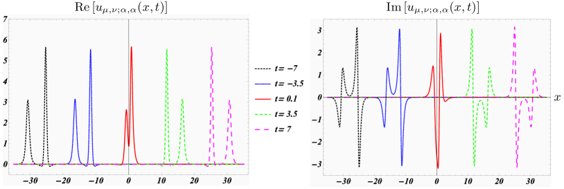
Figure 1: Degenerated KdV two-soliton compound solution with $\alpha=\beta=2$, $\mu=i\pi 3/5$ and $\nu=i\pi/5$ at different times.

As demonstrated in figure 2 this internal structure can be manipulated by varying the shift $\nu$.

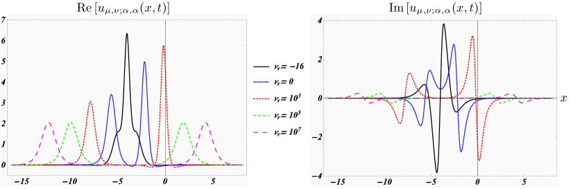
Figure 2: Degenerated KdV two-soliton compound solution with $\alpha=\beta=2$, $\nu=i\pi/5$ at fixed moment in time $t=-1$ and varying shift parameter $\nu=\nu_{r}+i\pi 3/5$.

For a fixed instance in time we can employ $\nu$ to increase or decrease the distance between the single soliton amplitudes and even find a value such that the distance becomes zero. However, this value is in the intermediate regime and as time evolves the two solitons will separate again to some finite distance in the asymptotic regime.

Our interpretation is supported by the computation of the energies resulting from (3) with Hamiltonian density (2) for the solution $u_{\mu,\nu;\alpha,\alpha}$. Numerically we find the finite real energies

$$E_{\mu,\nu;\alpha,\alpha}=\int\nolimits_{-\infty}^{\infty}{\mathcal{H}}[u_{\mu,\nu;\alpha,\alpha},(u_{\mu,\nu;\alpha,\alpha})_{x}]dx=-2\frac{\alpha^{5}}{5}=2E_{\mu;\alpha},$$ (30)

i.e. precisely twice the energy of the one-soliton $u_{\mu;\alpha}$, reported for instance in [12].

In order to compare with various other methods it is useful to note that the degenerate Wronskians may be obtained in several alternative ways. We conclude this subsection by reporting how the expression for the Wronskian (27) can be derived by mean of a limiting process directly from the two-soliton solution. This is seen from by starting from the defining relation for the Jordan state $\chi^{(1)}$

$$W\left[\psi_{\mu,\alpha},\chi_{\mu,\alpha}^{(1)}\right] = 2\lim_{\beta\rightarrow\alpha}\frac{\partial}{\partial\beta}W\left[\psi_{\mu,\alpha},\psi_{\mu,\beta}\right]$$ (31)

$$= 2\lim_{\beta\rightarrow\alpha}\lim_{h\rightarrow 0}W\left[\psi_{\mu,\alpha},\frac{\psi_{\mu,\beta+h}-\psi_{\mu,\beta}}{h}\right]$$ (32)

$$= 2\lim_{h\rightarrow 0}W\left[\psi_{\mu,\alpha},\frac{\psi_{\mu,\alpha+h}-\psi_{\mu,\alpha}}{h}\right]$$ (33)

$$= 2\lim_{h\rightarrow 0}\frac{1}{h}W\left[\psi_{\mu,\alpha},\psi_{\mu,\alpha+h}\right]$$ (34)

$$= 2\lim_{\beta\rightarrow\alpha}\frac{1}{\beta-\alpha}W\left[\psi_{\mu,\alpha},\psi_{\mu,\beta}\right],$$ (35)

where in the last step we chose $h=\beta-\alpha$. The shift can now be implemented by determining $\lambda$ from the limit of the expression

$$W\left[\psi_{\mu+\lambda\nu,\alpha},\psi_{\mu-\lambda\nu,\beta}\right] = W\left[\psi_{\mu,\alpha},\psi_{\mu,\beta}\right]\cosh^{2}\left(\frac{\lambda\nu}{2}\right)-W\left[\phi_{\mu,\alpha},\phi_{\mu,\beta}\right]\sinh^{2}\left(\frac{\lambda\nu}{2}\right)~{}~{}~{}~{}~{}~{}~{}~{}$$

$$+\frac{1}{2}\sinh\left(\lambda\nu\right)\left[W\left[\phi_{\mu,\alpha},\psi_{\mu,\beta}\right]-W\left[\psi_{\mu,\alpha},\phi_{\mu,\beta}\right]\right].$$

It it is obvious that for the limit (35) of the shifted expression to be finite we require $\lambda\sim(\alpha-\beta)$ with constant of proportionality chosen in such a way that it yields $1/2\alpha$ in the limit. Hence we obtain

$$W\left[\psi_{\mu,\alpha},\chi_{\mu,\alpha}^{(1)}+\frac{\nu}{\alpha}\phi_{\mu,\alpha}\right] = 2\lim_{\beta\rightarrow\alpha}\frac{1}{\beta-\alpha}W\left[\psi_{\mu+\frac{\alpha-\beta}{\alpha+\beta}\nu,\alpha},\psi_{\mu-\frac{\alpha-\beta}{\alpha+\beta}\nu,\beta}\right],$$ (37)

$$= 2\lim_{\beta\rightarrow\alpha}W_{\beta}\left[\psi_{\mu+\frac{\alpha-\beta}{\alpha+\beta}\nu,\alpha},\psi_{\mu-\frac{\alpha-\beta}{\alpha+\beta}\nu,\beta}\right].~{}$$ (38)

These identities will be useful below when we relate this approach to Hirota’s direct method.

2.2.2 Degenerate three-solitons

To find the degenerate three-soliton solution we may once again compute the Wronskian, albeit now involving two Jordan states. As discussed in the previous section, the expression for $W(\psi_{\mu,\alpha},\chi_{\mu,\alpha}^{(1)},\chi_{\mu,\alpha}^{(2)})$ will inevitably lead to solutions with infinite energy. Thus we will again exploit (5) with nonvanishing constants $c_{l}$, $d_{l}$ to generate the regularizing $\mathcal{PT}$-symmetric shifts. A suitable unique choice is

$$W\left[\psi_{\mu,\alpha},\chi_{\mu,\alpha}^{(1)}+\frac{\rho}{\alpha}\phi_{\mu,\alpha},\chi_{\mu,\alpha}^{(2)}+2\rho~{}\Omega_{\mu,\alpha}^{(1)}+\frac{2\nu-4\rho}{\alpha}\phi_{\mu,\alpha}\right]~{}~{}~{}~{}~{}~{}~{}\ \ ~{}~{}$$ (39)

$$= \alpha\left[1+\left(\eta_{\rho;\alpha}^{(3)}\right)^{2}+\cosh\left(\eta_{\mu;\alpha}^{(1)}\right)\right]\sinh\left(\frac{\eta_{\mu;\alpha}^{(1)}}{2}\right)-\alpha\eta_{\nu;\alpha}^{(9)}\cosh\left(\frac{\eta_{\mu;\alpha}^{(1)}}{2}\right),$$ (40)

where we abbreviated the different dispersion terms as

$$\eta_{\mu;\alpha}^{(\lambda)}:=\alpha x-\lambda\alpha^{3}t+\mu,$$ (41)

Notice that we have now three different shifted dispersion terms $\eta_{\mu;\alpha}^{(1)}$, $\eta_{\rho;\alpha}^{(3)}$ and $\eta_{\nu;\alpha}^{(9)}$, where the first governs the asymptotic behaviour and the remaining ones the additional structure in the intermediate regime. The solution $u_{\mu,\nu,\rho;\alpha,\alpha,\alpha}=2(\ln W)_{xx}$ is depicted in figure 3.

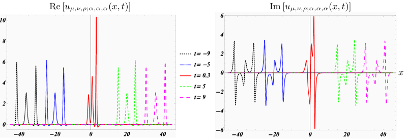
Figure 3: Degenerated KdV three-soliton compound solution with $\alpha=\beta=\gamma=2$, $\mu=i\pi 3/5$, $\nu=i\pi 3/10$ and $\rho=i\pi/10$.

We observe that asymptotically we have three single one-solitons moving at the same speed. They exchange their positions in the intermediate region near the origin, when the linear terms in (40) contribute.

For the general three-soliton solution we have also additional options available, namely to produce the degeneracy only in two of the one-solitons while keeping the remaining one at a different velocity. A suitable choice that produces the desired shifts is

$$W\left[\psi_{\mu,\alpha},\chi_{\mu,\alpha}^{(1)}+\frac{\nu}{\alpha}\phi_{\mu,\alpha},\psi_{\rho,\gamma}\right] = \left[\frac{\alpha^{2}+\gamma^{2}}{8}\sinh\left(\eta_{\mu;\alpha}^{(1)}\right)-\frac{\alpha^{2}-\gamma^{2}}{8}\eta_{\nu;\alpha}^{(3)}\right]\cosh\left(\frac{\eta_{\rho;\gamma}^{(1)}}{2}\right)$$ (42)

$$-\frac{\alpha\gamma}{2}\cosh^{2}\left(\frac{\eta_{\mu;\alpha}^{(1)}}{2}\right)\sinh\left(\frac{\eta_{\rho;\gamma}^{(1)}}{2}\right).$$

We depict the corresponding KdV solution $u_{\mu,\nu,\rho;\alpha,\alpha,\gamma}=2(\ln W)_{xx}$ in figure 4.

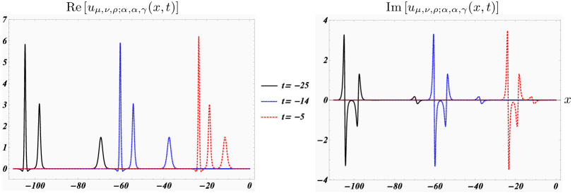
Figure 4: Degenerated KdV two-soliton compound solution scattering with a one-soliton with $\alpha=\beta=2$, $\gamma=1.7$, $\mu=i\pi 3/5$, $\nu=i\pi 3/10$ and $\rho=i\pi/10$.

We clearly observe that asymptotically we have a degenerated two-soliton and a one-soliton solution with the faster two-soliton overtaking the slower one-soliton.

Let us finish this section by reporting an alternative form of the degenerate three-soliton solution suitable for a comparison with other methods. We find

$$W\left[\psi_{\mu,\alpha},\chi_{\mu,\alpha}^{(1)}+\frac{\rho}{\alpha}\phi_{\mu,\alpha},\chi_{\mu,\alpha}^{(2)}+2\rho\Omega_{\mu,\alpha}^{(1)}+\frac{2\nu-4\rho}{\alpha}\phi_{\mu,\alpha}\right]$$ (43)

$$= 16\alpha\lim_{\gamma,\beta\rightarrow\alpha}\frac{1}{(\alpha-\beta)(\alpha-\gamma)(\gamma-\beta)}W\left[\psi_{\mu+f(\alpha,\beta,\gamma),\alpha},\psi_{\mu+f(\beta,\gamma,\alpha),\beta},\psi_{\mu+f(\gamma,\alpha,\beta),\gamma}\right]~{}~{}~{}~{}~{}~{}~{}\ \ ~{}~{}$$ (44)

$$= 8\alpha\lim_{\gamma,\beta\rightarrow\alpha}W_{\beta\gamma\gamma}\left[\psi_{\mu+f(\alpha,\beta,\gamma),\alpha},\psi_{\mu+f(\beta,\gamma,\alpha),\beta},\psi_{\mu+f(\gamma,\alpha,\beta),\gamma}\right],$$ (45)

where we introduced the shift function

$$f(x,y,z):=\frac{4}{9}\left[\frac{x^{2}+yz}{(x+y)(x+z)}-2\frac{x(y^{2}+z^{2})}{(x+y)(x+z)(y+z)}\right]\nu+\frac{4}{3}\frac{x^{2}-yz}{(x+y)(x+z)}\rho.$$ (46)

It will be important below to note that the sum of all shifts adds up to zero, $f(\alpha,\beta,\gamma)+f(\beta,\gamma,\alpha)+f(\gamma,\alpha,\beta)=0$.

Once again our interpretation is supported by the computation of the corresponding energies. Numerically we find

$$E_{\mu,\nu,\rho;\alpha,\alpha,\alpha} = \int\nolimits_{-\infty}^{\infty}{\mathcal{H}}[u_{\mu,\nu,\rho;\alpha,\alpha,\alpha},(u_{\mu,\nu,\rho;\alpha,\alpha,\alpha})_{x}]dx=-3\frac{\alpha^{5}}{5}=3E_{\mu;\alpha},$$ (47)

$$E_{\mu,\nu,\rho;\alpha,\alpha,\gamma} = \int\nolimits_{-\infty}^{\infty}{\mathcal{H}}[u_{\mu,\nu,\rho;\alpha,\alpha,\gamma},(u_{\mu,\nu,\rho;\alpha,\alpha,\gamma})_{x}]dx=-2\frac{\alpha^{5}}{5}-\frac{\gamma^{5}}{5}=2E_{\mu;\alpha}+E_{\mu;\gamma},~{}~{}~{}$$ (48)

which are again finite and real energies irrespective of whether the shifts are taken to be complex or real.

3 Degenerate complex multi-soliton solutions from Hirota’s direct method

Hirota’s direct method [18] takes a different equivalent form for nonlinear wave equations as starting point. The system at hand, the KdV equation (1), can be converted into Hirota’s bilinear form

$$\left(D_{x}^{4}+D_{x}D_{t}\right)\tau\cdot\tau=0,$$ (49)

by means of the variable transformation $u=2(\ln\tau)_{xx}$. The required combination of Hirota derivatives in terms of ordinary derivatives are

$$D_{x}^{4}\tau\cdot\tau = 2\tau_{xxxx}\tau-4\tau_{xxx}\tau_{x}+6\tau_{xx}\tau_{xx},$$ (50)

$$D_{x}D_{t}\tau\cdot\tau = 2\tau_{xt}\tau-2\tau_{x}\tau_{t}.$$ (51)

The $\tau$-function can be identified with the Wronskian in the previous section, up to the ambiguity of an overall factor $\exp\left[c_{1}x+c_{2}+f(t)\right]$ with arbitrary constants $c_{1}$, $c_{2}$ and function $f(t)$. Remarkably equation (49) can be solved with a perturbative Ansatz $\tau=\sum\nolimits_{k=0}^{\infty}\varepsilon^{k}\tau^{k}$ in an exact manner, meaning that this series terminates at $N$-th order in $\varepsilon$ for the corresponding $N$-soliton solution. Order by order one needs to solve the following set of linear equations

$$\left(D_{x}^{4}+D_{x}D_{t}\right)(1\cdot\tau^{1}+\tau^{1}\cdot 1) = 2(\tau^{1})_{xt}+2(\tau^{1})_{xxxx}=0,$$ (52)

$$\left(D_{x}^{4}+D_{x}D_{t}\right)(1\cdot\tau^{2}+\tau^{1}\cdot\tau^{1}+\tau^{2}\cdot 1) = 0,$$ (53)

$$\left(D_{x}^{4}+D_{x}D_{t}\right)(1\cdot\tau^{3}+\tau^{1}\cdot\tau^{2}+\tau^{2}\cdot\tau^{1}+\tau^{3}\cdot 1) = 0.$$ (54)

Let us first see how the Hirota equations are solved using Wronskians involving Jordan states. We start with the two-soliton solution and take $\tau^{1}=W_{x}\left[\psi,\chi^{(1)}\right]$. Using identity (7) in the form $W_{x}\left[\psi,\chi^{(1)}\right]=c\psi^{2}$, the first order Hirota equation (52) reads

$$(\tau^{1})_{xt}+(\tau^{1})_{xxxx}=(W_{x})_{t}+(W_{x})_{xxx}=c(\psi^{2})_{t}+c(\psi^{2})_{xxx}=2c\psi\left(\psi_{t}+\alpha^{2}\psi_{x}\right)=0.$$ (55)

This equation is solved using the above mentioned nonlinear dispersion relation, i.e. by taking $\psi(x,t)=\psi(x-\alpha^{2}t)$.

Next we show how one may carry out the limit to our degenerate solutions directly on the Hirota multi-soliton solutions. The two-soliton $\tau$-function is known to be of the form

$$\tau_{\alpha,\beta}(x,t)=1+c_{1}e^{\eta_{a}}+c_{2}e^{\eta_{\beta}}+c_{1}c_{2}\varkappa(\alpha,\beta)e^{\eta_{a}+\eta_{\beta}}$$ (56)

with $\eta_{a}:=\alpha x-\alpha^{3}t$ and $\varkappa(\alpha,\beta):=$ $(\alpha-\beta)^{2}/(\alpha+\beta)^{2}$. Usually the constants $c_{1}$ and $c_{2}$ are set to one. Evidently carrying out the limit  $\alpha\rightarrow\beta$ in this variant will simply produce a one-soliton solution. However, when making use of the freedom to multiply the $\tau$-function with an overall factor we define

$$\tau_{\mu,\nu;\alpha,\beta}(x,t)=\frac{8}{(\alpha-\beta)}e^{\frac{\eta_{a}+\eta_{\beta}}{2}+\mu}W\left[\psi_{\mu+\frac{\alpha-\beta}{\alpha+\beta}\nu,\alpha},\psi_{\mu-\frac{\alpha-\beta}{\alpha+\beta}\nu,\beta}\right],$$ (57)

which produces the series expansion form (56) of the $\tau$-function with coefficients

$$c_{1}=-\frac{\alpha+\beta}{\alpha-\beta}e^{\mu+\frac{\alpha-\beta}{\alpha+\beta}\nu},\qquad\text{and\qquad}c_{2}=\frac{\alpha+\beta}{\alpha-\beta}e^{\mu-\frac{\alpha-\beta}{\alpha+\beta}\nu}.$$ (58)

In this form the limit is easily performed

$$\tau_{\mu,\nu;\alpha,\alpha}(x,t)=\lim_{\beta\rightarrow\alpha}\tau_{\mu,\nu;\alpha,\beta}(x,t)=1-2(\alpha x-3\alpha^{3}t+\nu)e^{\eta_{a}+\mu}-e^{2\eta_{a}+2\mu}.$$ (59)

Since the factor in (57) has the form of the general ambiguity, the expression $2\left(\ln\tau_{\mu,\nu;\alpha,\alpha}\right)_{xx}$ produces the same two-soliton solution (28) as previously obtained.

Similarly, using the identity

$$\tau_{\mu,\nu,\rho;\alpha,\beta,\gamma}(x,t)=\frac{64\exp\left(\frac{\eta_{a}+\eta_{\beta}+\eta_{\gamma}+3\mu}{2}\right)}{(\alpha-\beta)(\alpha-\gamma)(\beta-\gamma)}W\left[\psi_{\mu+f(\alpha,\beta,\gamma),\alpha},\psi_{\mu+f(\beta,\gamma,\alpha),\beta},\psi_{\mu+f(\gamma,\alpha,\beta),\gamma}\right]$$ (60)

we obtain the series expansion form (56) of the $\tau$-function for the 3-soliton solution

$$\tau_{\mu,\nu,\rho;\alpha,\beta,\gamma}(x,t) = 1+c_{1}e^{\eta_{a}}+c_{2}e^{\eta_{\beta}}+c_{3}e^{\eta_{\gamma}}+c_{1}c_{2}\varkappa(\alpha,\beta)e^{\eta_{a}+\eta_{\beta}}+c_{1}c_{3}\varkappa(\alpha,\gamma)e^{\eta_{a}+\eta_{\gamma}}$$ (61)

$$+c_{2}c_{3}\varkappa(\beta,\gamma)e^{\eta_{\beta}+\eta_{\gamma}}+c_{1}c_{2}c_{3}\varkappa(\alpha,\beta)\varkappa(\alpha,\gamma)\varkappa(\beta,\gamma)e^{\eta_{a}+\eta_{\beta}+\eta_{\gamma}}$$

with coefficients

$$c_{1}=c(\alpha,\beta,\gamma),\quad c_{2}=c(\beta,\gamma,\alpha),\quad c_{3}=c(\gamma,\alpha,\beta),~{}~{}$$ (62)

where

$$c(x,y,z)=\frac{(x+y)(x+z)}{(x-y)(x-z)}e^{\mu+f(x,y,z)}.$$ (63)

Clearly without the information from the previous section it is not obvious at this stage how to determine the coefficients $c_{i}$ in general, especially the regularizing shifts.

4 Degenerate complex multi-soliton solutions from superposition

It is well-known that the combination of four Bäcklund transformations combined in a Bianchi-Lamb [21, 22] commutative fashion gives rise to a “nonlinear superposition principle”, e.g. [12]. Introducing the quantity $u=w_{x}$, it takes on the form

$$w_{12}=w_{0}+2\frac{\kappa_{1}-\kappa_{2}}{w_{1}-w_{2}},$$ (64)

for the KdV equation where $w_{0}$, $w_{1}$, $w_{2}$ and $w_{12}$ correspond to different solutions. Relating $w_{1}$ and $w_{2}$ to the standard one-soliton solution and setting $w_{0}$ to the trivial solution $w_{0}=0$, the general formula (64) becomes

$$w_{\mu,\hat{\mu};\alpha,\beta}=\frac{\alpha^{2}-\beta^{2}}{w_{\mu;\alpha}-w_{\hat{\mu};\beta}},$$ (65)

with $w_{\mu;\alpha}(x,t)=\alpha\tanh\left[\frac{1}{2}(\alpha x-\alpha^{3}t+\mu)\right]$, $\kappa_{1}=\alpha^{2}/2$ and $\kappa_{2}=\beta^{2}/2$, see [12]. Remarkably in this form the limit $\lim_{\beta\rightarrow\alpha}w_{\mu,\hat{\mu};\alpha,\beta}$ can be performed directly

$$\lim_{\beta\rightarrow\alpha}w_{\mu,\hat{\mu};\alpha,\beta}=\left\{\begin{array}[]{cc}0&\text{for }\mu\neq\hat{\mu}\\ 2\alpha\frac{1+\cosh\left(\eta_{\mu;\alpha}^{(1)}\right)}{\eta_{0;\alpha}^{(3)}+\sinh\left(\eta_{\mu;\alpha}^{(1)}\right)}{}{}{}{}&\text{for }\mu=\hat{\mu}\end{array}\right..$$ (66)

The corresponding solution the KdV equation will still be singular, but when implementing the same shifts as in (37) we compute

$$\left(\lim_{\beta\rightarrow\alpha}w_{\mu+\frac{\alpha-\beta}{\alpha+\beta}\nu,\mu-\frac{\alpha-\beta}{\alpha+\beta}\nu;\alpha,\beta}\right)_{x}=\lim_{\beta\rightarrow\alpha}\left(w_{\mu+\frac{\alpha-\beta}{\alpha+\beta}\nu,\mu-\frac{\alpha-\beta}{\alpha+\beta}\nu;\alpha,\beta}\right)_{x}=u_{\mu,\nu;\alpha,\alpha},$$ (67)

and thus recover precisely the solution (28). The relation to the treatment in section 2 involving DC–transformations is achieved by considering (14) for $n=0$ with $V^{(0)}=0$. Then we read off the identification $w_{\mu;\alpha}=2\left(\ln\psi_{\mu,\alpha}\right)_{x}$, which is confirmed by the explicit expression (19).

Similarly we may carry out the limit on higher soliton solutions. For instance, iterating (64) once more we obtain the three-soliton solution

$$w_{\mu,\nu,\rho;\alpha,\beta,\gamma}=w_{\mu;\alpha}+\frac{\beta^{2}-\gamma^{2}}{w_{\mu,\nu;\alpha,\beta}-w_{\mu,\rho;\alpha,\gamma}},$$ (68)

which yields the non-trivial limit

$$\lim_{\beta,\gamma\rightarrow\alpha}w_{\mu,\mu,\mu;\alpha,\beta,\gamma}=\frac{2\left[\left[1+\left(\eta_{0;\alpha}^{(3)}\right)^{2}+\cosh\left(\eta_{\mu;\alpha}^{(1)}\right)\right]\sinh\left(\frac{\eta_{\mu;\alpha}^{(1)}}{2}\right)-\eta_{0;\alpha}^{(9)}\cosh\left(\frac{\eta_{\mu;\alpha}^{(1)}}{2}\right)\right]_{x}}{\left[1+\left(\eta_{0;\alpha}^{(3)}\right)^{2}+\cosh\left(\eta_{\mu;\alpha}^{(1)}\right)\right]\sinh\left(\frac{\eta_{\mu;\alpha}^{(1)}}{2}\right)-\eta_{0;\alpha}^{(9)}\cosh\left(\frac{\eta_{\mu;\alpha}^{(1)}}{2}\right)}.$$ (69)

When implementing the appropriate shifts and differentiating once more this produces precisely the same three-soliton solution as previously constructed in section 2.2.2.

5 Conclusions

We have constructed a novel type of compound soliton solution composed of a fixed number degenerate one-soliton constituents with the same energy. Asymptotically, that is for large and small time, the individual one-solitons travel at the same velocity with almost constant amplitudes. In the intermediate regime they scatter and exchange their relative position. Thus the entire collection of one solitons may be viewed as a single compound object with an internal structure only visible in a certain regime of time. As we have shown, one may construct solutions in which these compounds scatter with other (degenerate) multi-solitons at different velocities.

Technically these compound structures arose from carefully designed limiting processes of multi-soliton solutions. We have demonstrated how these limits can be performed within the context of standard techniques of integrable systems, employing Darboux-Crum transformations involving Jordan states, Hirota’s direct method with specially selected coefficients and on the nonlinear superposition obtained from Bäcklund transformations. While the limits led to mathematically admissible nonlinear wave solutions, they always possess singularities such that their energy becomes infinite. In order to convert them into physical objects it was crucial to implement in addition some complex regularizing shifts.

When comparing the different methods, the DC-transformations require the most substantial modification by the introduction of Jordan states. This approach is very systematic and the modified transformations always constitute degenerate soliton solutions. To carry out the limit within the context of Hirota’s direct method requires some guesswork in regards to the appropriate choice of coefficients, which we overcame here by relying on the information from the DC-transformations. The nonlinear superposition of three solutions appears to be the most conductive form for taking the limit directly. The disadvantage in this approach is that expressions for higher multi-soliton solutions are rather cumbersome when expressed iteratively. So far in all approaches the regularizing shift were introduced in a somewhat ad hoc fashion.

There are various open issues left to be resolved and not reported here. Evidently the suggested procedure is entirely generic and not limited to the KdV equations or the particular type of solutions and boundary conditions considered here [23]. It would be interesting to apply them to other types of integrable systems as that might help to unravel some further universal features. For instance, one expects that the regularizing shifts can be cast into a more universal form that might be valid for any arbitrary number of degeneracies when exploiting further their ambiguities. Furthermore it is desirable to complete the argument on why the energies of these complex solutions are real. This follows immediately when they and the corresponding Hamiltonians are $\mathcal{PT}$-symmetric. As demonstrated in [12], this can be achieved with suitable real shifts in time or space, but in addition one also requires the model to be integrable. We report on these issues in more detail elsewhere [24].

Acknowledgments: FC would like to thank the Alexander von Humboldt Foundation (grant number CHL 1153844 STP) for financial support and City University London for kind hospitality.

References

• [1] P. J. Olver and D. H. Sattinger, Solitons in physics, mathematics, and nonlinear optics, Springer Science & Business Media 25 (2012).
• [2] J. E. Bjorkholm and A. A. Ashkin, CW self-focusing and self-trapping of light in sodium vapor, Phys. Rev. Lett. 32(4), 129 (1974).
• [3] J. von Neuman and E. Wigner, Über merkwürdige diskrete Eigenwerte. Über das Verhalten von Eigenwerten bei adiabatischen Prozessen, Zeit. der Physik 30, 467–470 (1929).
• [4] M. Kovalyov, On a class of solutions of KdV, Journal of Differential Equations 213(1), 1–80 (2005).
• [5] M. Kovalyov, On a class of solutions of the sine-Gordon equation, Journal of Physics A: Mathematical and Theoretical 42(49), 495207 (2009).
• [6] C. M. Bender and S. Boettcher, Real Spectra in Non-Hermitian Hamiltonians Having PT Symmetry, Phys. Rev. Lett. 80, 5243–5246 (1998).
• [7] C. M. Bender, Making sense of non-Hermitian Hamiltonians, Rept. Prog. Phys. 70, 947–1018 (2007).
• [8] A. Mostafazadeh, Pseudo-Hermitian Representation of Quantum Mechanics, Int. J. Geom. Meth. Mod. Phys. 7, 1191–1306 (2010).
• [9] Z. H. Musslimani, K. G. Makris, R. El-Ganainy, and D. N. Christodoulides, Optical Solitons in PT Periodic Potentials, Phys. Rev. Lett. 100, 030402 (2008).
• [10] K. G. Makris, R. El-Ganainy, D. N. Christodoulides, and Z. H. Musslimani, PT-symmetric optical lattices, Phys. Rev. A81, 063807(10) (2010).
• [11] A. Guo, G. J. Salamo, D. Duchesne, R. Morandotti, M. Volatier-Ravat, V. Aimez, G. A. Siviloglou, and D. Christodoulides, Observation of PT-Symmetry Breaking in Complex Optical Potentials, Phys. Rev. Lett. 103, 093902(4) (2009).
• [12] J. Cen and A. Fring, Complex solitons with real energies, arXiv preprint arXiv:1602.05465 (2016).
• [13] F. Correa, V. Jakubskỳ, and M. S. Plyushchay, PT-symmetric invisible defects and confluent Darboux-Crum transformations, Physical Review A 92(2), 023839 (2015).
• [14] G. Darboux, On a proposition relative to linear equations, physics/9908003, Comptes Rendus Acad. Sci. Paris 94, 1456–59 (1882).
• [15] M. M. Crum, Associated Sturm-Liouville systems, The Quarterly Journal of Mathematics 6(1), 121–127 (1955).
• [16] V. B. Matveev, Asymptotics of the multipositon–soliton $\tau$ function of the Korteweg–de Vries equation and the supertransparency, Journal of Mathematical Physics 35(6), 2955–2970 (1994).
• [17] V. B. Matveev and M. A. Salle, Darboux transformation and solitons, (Springer, Berlin) (1991).
• [18] R. Hirota, Exact Solution of the Korteweg-de Vries Equation for Multiple Collisions of Solitons, Phys. Rev. Lett. 27, 1192 – 1194 (1971).
• [19] D. J. Korteweg and deVries G., On the change of form of long waves advancing in a rectangular canal, and on a new type of long stationary waves, Phil. Mag. 39, 422–443 (1895).
• [20] A. Fring, $\cal{PT}$-Symmetric deformations of the Korteweg-de Vries equation, J. Phys. A 40, 4215–4224 (2007).
• [21] G. L. Lamb Jr, Analytical descriptions of ultrashort optical pulse propagation in a resonant medium, Reviews of Modern Physics 43, 99–124 (1971).
• [22] L. Bianchi, Vorlesungen über Differentialgeometrie, (Teubner, Leipzig) (1927).
• [23] A. Arancibia and M. S. Plyushchay, Chiral asymmetry in propagation of soliton defects in crystalline backgrounds, Physical Review D 92(10), 105009 (2015).
• [24] J. Cen, F. Correa, and A. Fring, in preparation.