Exciton absorption in narrow armchair graphene nanoribbons

Abstract

We develop an analytical approach to the exciton optical absorption for narrow gap armchair graphene nanoribbons (AGNR). We focus on the regime of dominant size quantization in combination with the attractive electron-hole interaction. An adiabatic separation of slow and fast motions leads via the two-body Dirac equation to the isolated and coupled subband approximations. Discrete and continuous exciton states are in general coupled and form quasi Rydberg series of purely discrete and resonance type character. Corresponding oscillator strengths and widths are derived. We show that the exciton peaks are blue-shifted, become broader and increase in magnitude upon narrowing the ribbon. At the edge of a subband the singularity related to the 1D density of states is transformed into finite absorption via the presence of the exciton. Our analytical results are in good agreement with those obtained by other methods including numerical approaches. Estimates of the expected experimental values are provided for realistic AGNRs.

I Introduction

Spatially confined elongated strips of graphene monolayer termed graphene nanoribbons (GNR) have attracted in recent years substantial interest both theoretically and experimentally (see Wakab ; Alf ; Soavi and references therein). GNR are of fundamental importance for nanoscience and nanotechnology applications. In general, surpass the gapless 2D graphene monolayers with fixed electronic, optical, and transport properties, and demonstrate flexible features because of an open tunable electronic band gap governed by the ribbon width. In contrast to zigzag GNR, the armchair GNR (AGNR), which possess extrema of the energy bands at the common centre of the Brillouin zone are more amenable to a theoretical description. Below we will focus on the semiconductor-like quasi-1D AGNR having open band gaps $\Delta_{N_{eh}}=\varepsilon_{N_{e}}-\varepsilon_{N_{h}}$ determined by the distances between the electron $(e)$ and hole $(h)$ size-quantized energy levels $\varepsilon_{N_{e,h}}\sim d^{-1}$ induced by a finite ribbon width $d$.

Optical absorption caused by the transitions between the electron and hole subbands associated with the energy levels $\varepsilon_{N_{e,h}}$ represents an effective tool to explore the electronic structure of the AGNR electronic structure. The key point is the inverse square-root divergence of the density of 1D states of free carriers at the band gaps, manifesting itself in the inter-subband optical effects. However, in the experimental spectra of real AGNR these singularities are replaced by a more complicated pattern. Excitons formed by the attractively interesting electron and hole drastically change the optical absorption properties in the vicinity of the edges determined by the energy gaps. It was shown for exciton absorption in a bulk semiconductor subject to a strong magnetic field Hashow and in a narrow semiconductor quantum wire Monschm09 that Rydberg series of exciton peaks arise below each edge and tend to a finite absorption at edges thereby shadowing the square-root singularity and modifying the fundamental absorption above the edges. In addition, quasi-1D semiconductor structures are preferable for exciton studies. In units of the exciton Rydberg constant $Ry^{\mbox{\tiny(x)}}$ the exciton binding energy $E_{b}$ in a 3D bulk material is $E_{b}^{(3\mbox{\tiny D})}=Ry^{\mbox{\tiny(x)}}$, in a 2D quantum well $E_{b}^{(2\mbox{\tiny D})}=4Ry^{\mbox{\tiny(x)}}$, while in a 1D quantum wire it is suppressed both by a magnetic field or by the boundaries of the wire $E_{b}^{(1\mbox{\tiny D})}\sim Ry^{\mbox{\tiny(x)}}\ln^{2}(\frac{R}{a_{\mbox{\tiny x}}})$,  ($R<<a_{\mbox{\tiny x}}$), where $R$ is the wire radius or the magnetic length. In this sense the AGNR surpass the semiconductor structures for which the Rydberg constant is a fixed parameter, while for the AGNR $Ry^{\mbox{\tiny(x)}}\sim\Delta_{N_{eh}}\sim d^{-1}$ Nov ; Monschm12 .

To date, the discrete part of the exciton absorption spectrum of GNR has been calculated numerically Yang ; Prez ; Zhu ; Denk using approaches based on density functional theory, the local density approximation, and the Bethe-Salpeter equation. Jia et al. Jia and Lu et al. Lu used the tight-binding approximation, while Alfonsi and Meneghetti Alf employed the Hubbard Hamiltonian in their ab initio calculations of the positions and intensities of the exciton peaks. Only a few of the recent approaches Rat ; Mohamm relied on analytical methods based on the nonrelativistic Wannier 1D model. Thus, by now the absolute majority of the works focusing on the problem of exciton absorption in narrow AGNR are numerical calculations aiming at the exciton binding energy or and discrete exciton peaks. A consistent analytical theory, that considers the 2D two-body exciton Hamiltonian and gives rise to quasi-1D bound and unbound excitons, inducing discrete and continuous optical absorption, respectively, is virtually not addressed in the literature. The inter-subband interaction of the exciton states did not yet attract attention. In addition, the complete form of the exciton absorption coefficient has not been derived explicitly. Undoubtedly, numerical calculations are required for an adequate description of concrete experiments. Nevertheless, analytical methods are indispensable to make the basic physics of AGNR transparent and then to promote the application of these materials in nano- and opto-electronics using the dependence of the properties of the AGNR on the ribbon width.

In order to fill the mentioned gaps we develop an analytical approach, which yields an explicit form of the exciton absorption coefficient for AGNR. The electron-hole Coulomb attraction is taken to be much weaker than the effect of the ribbon confinement, which in turn means a narrow ribbon as compared to the exciton Bohr radius. The two-body Dirac equation describing the 2D massless electron-hole pair is solved in the adiabatic approximation. This approximation implies that the transverse motion of the particles governed by the ribbon confinement is much faster than its longitudinal motion controlled by the 1D exciton field, which is calculated by averaging the 2D Coulomb exciton potential over the electron and hole transverse states. In the single-subband approximation of isolated $N$-subbands the exciton energy spectrum is a sequence of series of the quasi-Coulomb strictly discrete $Nn$- levels positioned below the $N$th size-quantized level and continuous subbands originating from each $N$-level. A coupling between the discrete and continuous exciton states, specified by the $N=0,1$ levels is taken into account in the double-subband approximation. Inter-subband interaction converts the strictly discrete $Nn$-states into the quasi-discrete ones (Fano resonances), having nonzero energy widths, which manifest itself in the Lorentzian form of the exciton absorption peaks. Clearly, energetically lowest exciton series, corresponding to the ground size-quantized level $N=0$ does not interact with the series lying above and remains discrete.

Our mathematical approach is based on matching the Coulomb wave functions with the functions obtained upon solution of the Dirac equation in the intermediate region by the iteration method. This procedure has been originally developed by Hasegawa and Howard Hashow for 3D excitons subject to a strong magnetic field and then successfully extended to problems related to semiconductor (see Monschm09 and references therein) and graphene Monschm12 ; Monschm14 nanostructures. The dependence of the exciton absorption coefficient on the ribbon width is studied analytically. Our results are in line with the conclusions based on numerical approaches and the corresponding experimental data. The aim of this work is to make AGNR attractive as optoelectronic devices due to the strong dependence of the exciton spectrum on the ribbon width.

This work is organized as follows. In Section 2 the general analytical approach is described. The energy levels of the discrete states and the exciton wave functions of the discrete and continuous energy spectrum are calculated in Section 3 in the single-subband approximation. The discrete exciton peaks and the continuous absorption are considered in Section 4. Section 5 provides the double-subband approximation to study the optical series of the Fano $n$-resonances, relevant to the first excited subband $N=1.$ In Section 6 we discuss the obtained results, compare them with the available data, and estimate the expected experimental values. Section 7 contains our conclusions.

II General approach

Below we consider the exciton absorption in an AGNR with width $d$ and length $L$ placed on the $x-y$ plane and bounded by straight lines $x=\pm d/2.$ The polarization of the light wave is assumed to be parallel to the $y$-axis. Optical absorption in GNR associated with electron interband transitions has been studied numerically by Hsu and Reichl Hsu as well as Gundra and Shukla Gund , while a comprehensive analytical approach was recently developed by Sasaki et al Sas . In particular, it was shown that the inter-subband $y$-polarized transitions are allowed between the electron $N_{e}$ and the hole $N_{h}$ subbands with the same indices $N_{e}=N_{h}=N$. Elliot justified thoroughly in Ref. Ell that the exciton absorption in semiconductors, can be treated as the electron-hole pair optical transition from the ground state described by the wave function $\Psi^{(0)}(\vec{\rho}_{e},\vec{\rho}_{h})$ to the excited exciton state $\Psi^{\mbox{\tiny}(x)}(\vec{\rho}_{e},\vec{\rho}_{h})$, in which the electron $(e)$ and hole $(h)$ with coordinates $\vec{\rho}_{e}$ and $\vec{\rho}_{h}$ are in the conduction and valence band, respectively. On extending the results of Elliot Ell and Sasaki et al. Sas to exciton transitions in a semiconductor-like AGNR, the exciton absorption coefficient $\alpha$ becomes

$$\alpha=\sum_{N}\alpha^{(N)};\quad\alpha^{(N)}=\frac{1}{n_{b}\varepsilon_{0}c}\sigma_{yy}^{(N)},$$ (1)

where $\sigma_{yy}^{(N)}$ is the component of the dynamical conductivity

$$\sigma_{yy}^{(N)}=\frac{\pi p^{2}e^{2}}{\hbar S\Delta_{N}}\sum_{n,s}\big{|}\sigma^{(N)}_{xn(s)}\big{|}^{2}\delta\left(\hbar\omega-E_{Nn(s)}\right)\delta_{\vec{q}_{ph}\vec{K}}$$ (2)

determined by the matrix element

$$\sigma^{(N)}_{xn(s)}=\left<\vec{\Psi}^{(0)}(\vec{\rho}_{e},\vec{\rho}_{h})|\hat{\sigma}_{xh}\bigotimes\hat{I}_{e}+\hat{I}_{h}\bigotimes\hat{\sigma}_{xe}|\vec{\Psi}^{(\mbox{ex})}_{Nn(s)}(\vec{\rho}_{e},\vec{\rho}_{h})\right>$$ (3)

of the Pauli matrix $\hat{\sigma}_{x}$ calculated between the ground $\vec{\Psi}^{(0)}$ and exciton $\vec{\Psi}^{\mbox{\tiny(x)}}_{Nn(s)}$ wave vectors of the bound $(n)$ and continuous $(s)$ states of the exciton, formed by an electron and hole from the corresponding energy subbands with the common index $N$. As usual, the symbol $\bigotimes$ denotes the tensor product of the Pauli $\hat{\sigma}_{x}$ and unit $\hat{I}$ matrices. In eq. (1) $n_{b}$ is the refraction index of the ribbon substrate, $c$ is the speed of light, while in eq. (2) $p=\hbar v_{F},~{}(v_{F}=10^{6}\,\mbox{m/s})$ is the graphene energy parameter , $S=Ld$ is the area of the ribbon, $\Delta_{N}=2\varepsilon_{N}$ is the effective energy gap between the electron and hole subbands, branching from the size-quantized levels $\pm\varepsilon_{N}$ in conduction and valence bands, respectively. The $\delta$-functions in eq. (2) reflect the conservation laws in the system formed by the absorbed photon with the energy $\hbar\omega$ and momentum $\hbar\vec{q}_{\mbox{\tiny{ph}}}$ plus emersed exciton of the energy $E_{Nn(s)}$ and the total momentum $\hbar\vec{K}$.

Following Elliott’s approach Ell the wave function $\vec{\Psi}^{(0)}$ related to the ground state of the electron-hole pair in an AGNR can be chosen in the form

$$\vec{\Psi}^{(0)}(\vec{\rho}_{e},\vec{\rho}_{h})=\delta(y)\delta(x_{e}-x_{h})\left[\vec{\Phi}_{A}^{(0)}(x_{e})\bigotimes\vec{\Phi}_{A}^{(0)}(x_{h})+\vec{\Phi}_{B}^{(0)}(x_{e})\bigotimes\vec{\Phi}_{B}^{(0)}(x_{h})\right],$$ (4)

where $y=y_{e}-y_{h}$ is the relative $y$-coordinate and

$$\vec{\Phi}_{A}^{(0)}(x)=\frac{1}{\sqrt{2}}\begin{array}[]{c}\begin{Bmatrix}-1\\ 0\\ 1\\ 0\end{Bmatrix}\end{array};\qquad\vec{\Phi}_{B}^{(0)}(x)=\frac{1}{\sqrt{2}}\begin{array}[]{c}\begin{Bmatrix}0\\ 1\\ 0\\ -1\end{Bmatrix}\end{array}.$$

The exciton wave function $\vec{\Psi}^{\mbox{\tiny(x)}}$ can be found by solving the equation

$$\hat{{\rm H}}_{\mbox{\tiny x}}\vec{\Psi}^{\mbox{\tiny(x)}}(\vec{\rho_{e}},\vec{\rho_{h}})=E\vec{\Psi}^{\mbox{\tiny(x)}}(\vec{\rho_{e}},\vec{\rho_{h}}).$$ (5)

In this equation

$$\hat{{\rm H}}_{\mbox{\tiny x}}=\hat{{\rm H}}_{h}(\hat{\vec{k}}_{h})\bigotimes\hat{I}_{e}+\hat{I}_{h}\bigotimes\hat{{\rm H}}_{e}(\hat{\vec{k}}_{e})+\hat{I}_{h}\bigotimes\hat{I}_{e}V(\vec{\rho_{e}}-\vec{\rho_{h}})$$ (6)

is the traditional exciton Hamiltonian Mohen formed by the electron and hole Hamiltonians $\hat{{\rm H}}_{j}(\hat{\vec{k}}_{j}),~{}j=e,h$ corresponding to the nonequivalent Dirac points
$\vec{K}^{(+,-)}=\pm K,0;~{}(K=4\pi/3a_{0},~{}a_{0}=2.46\,\mbox{{\AA}}$ is the graphene lattice constant). The Hamiltonian $\hat{{\rm H}}_{j}(\hat{\vec{k}}_{j})$ is represented by Monschm12 ; Brfer

$$\hat{{\rm H}}_{j}(\vec{k}_{j})=p\left(\begin{array}[]{cc}-\vec{\sigma}\hat{\vec{k}}_{j}&0\\ 0&\vec{\sigma}^{*}\hat{\vec{k}}_{j}\\ \end{array}\right);\qquad\hat{\vec{k}}_{j}=-i\vec{\nabla}_{j};$$

containing the Pauli matrices $\sigma_{x,y}$, unit matrices $\hat{I}_{j},~{}j=e,h$ and the 2D Coulomb potential of the electron-hole attraction

$$V(\vec{\rho}_{e},\vec{\rho}_{h})=-\frac{e^{2}}{4\pi\varepsilon_{0}\epsilon_{\mbox{\tiny eff}}\sqrt{(x_{e}-x_{h})^{2}+(y_{e}-y_{h})^{2}}}.$$ (7)

Here $\epsilon_{\mbox{\tiny eff}}=\frac{1}{2}(1+\epsilon+\pi q_{0})$ is the effective dielectric constant determined by the static dielectric constant $\epsilon$ of the substrate and by the parameter $q_{0}=e^{2}/4\pi\varepsilon_{0}p\simeq 2.2$ Nov ; Hwang .

Further we choose the exciton wave function $\vec{\Psi}^{\mbox{\tiny(x)}}$ in the form

$$\vec{\Psi}^{\mbox{\tiny(x)}}(\vec{\rho_{e}},\vec{\rho_{h}})=\sum_{N}\vec{\Psi}_{N}^{\mbox{\tiny(x)}}(\vec{\rho_{e}},\vec{\rho_{h}})$$ (8)

where

$$\vec{\Psi}_{N}^{\mbox{\tiny(x)}}(\vec{\rho_{e}},\vec{\rho_{h}})=\vec{\Psi}_{N}(\vec{\rho_{h}})\bigotimes\vec{\Psi}_{N}(\vec{\rho_{e}}),$$

and where

$$\vec{\Psi}_{N}(\vec{\rho}_{j})=\frac{1}{\sqrt{2}}\left[u_{NA}(y_{j})\vec{\Phi}_{NA}(x_{j})+u_{NB}(y_{j})\vec{\Phi}_{NB}(x_{j})\right];\quad j=e,h.$$ (9)

are the single particle wave-functions both related to the $N$ subband. The exciton states consisting of the electron and the hole associated with the different $N_{e}\neq N_{h}$ subbands are optically inactive and can be excluded from the expansion (9) (see Monschm05 and references therein).

In equation (9) the sublattice wave functions $\vec{\Phi}_{NA,B}$ are as follows

$$\vec{\Phi}_{NA}(x_{j})=\begin{array}[]{c}\begin{Bmatrix}-\varphi_{N}(x_{j})\\ 0\\ \varphi_{N}^{\ast}(x_{j})\\ 0\end{Bmatrix}\end{array};\qquad\vec{\Phi}_{NB}(x_{j})=\begin{array}[]{c}\begin{Bmatrix}0\\ \varphi_{N}(x_{j})\\ 0\\ -\varphi_{N}^{\ast}(x_{j})\end{Bmatrix}\end{array};\quad j=e,h$$

where the functions $\varphi_{N}(x_{j})$ are represented by

$$\varphi_{N}(x_{j})=\frac{1}{\sqrt{2d}}\exp\left\{{\rm i}\left[x_{j}\frac{\pi}{d}(N-\tilde{\sigma})-\frac{\pi}{2}\left(N+\left[\frac{Kd}{\pi}\right]\right)\right]\right\}.$$ (10)

These wave functions form the single particle orthonormal wave functions Monschm12

$$\vec{\Phi}_{N}(x_{j})=\frac{1}{\sqrt{2}}\left[\vec{\Phi}_{NA}(x_{j})+\vec{\Phi}_{NB}(x_{j})\right]~{};$$ (11)

satisfying the equations

$$\langle\vec{\Phi}_{N^{\prime}B,A}|\vec{\Phi}_{NA,B}\rangle=0~{};\quad\langle\vec{\Phi}_{N^{\prime}A,B}|\vec{\Phi}_{NA,B}\rangle=\langle\vec{\Phi}_{N^{\prime}}|\vec{\Phi}_{N}\rangle=\delta_{N^{\prime}N}.$$

The introduced wave functions obey the equations

$$\left.\begin{array}[]{c}\hat{H}_{j}(\hat{k}_{jx},0)\vec{\Phi}_{N}(x_{j})=\varepsilon_{N}\vec{\Phi}_{N}(x_{j});\\ \hat{H}_{j}(\hat{k}_{jx},0)\vec{\Phi}_{NA,B}(x_{j})=\varepsilon_{N}\vec{\Phi}_{NB,A}(x_{j});\\ \varepsilon_{N}=|N-\tilde{\sigma}|\frac{\pi p}{d};~{}N=0,\pm 1,\pm 2,\ldots~{};\quad\tilde{\sigma}=\frac{Kd}{\pi}-\left[\frac{Kd}{\pi}\right]~{};\,j=e,h~{};\end{array}\right\}$$ (15)

Below to be specific we will consider AGNR of the family sigma = 1/3, providing a semiconductor-like gap structure, and we leave aside the case sigma = 0 corresponding to the metall-like gapless ribbon.

The components $\varphi_{N}(x_{j}),\,(j=e,h)$ in (10) and energies $\varepsilon_{N}$ in eq. (15) have been derived from the boundary conditions

$${\rm e}^{{\rm i}Kx_{j}}\varphi_{N}(x_{j})-{\rm e}^{-{\rm i}Kx_{j}}\varphi^{*}_{N}(x_{j})=0\quad\mbox{at}\quad x_{j}=\pm\frac{d}{2};~{}j=e,h,$$ (16)

which provide that the electron $(e)$ and hole $(h)$ states $\vec{\Phi}_{NA,B}$ multiplied by the factor $\exp\left[{\rm i}\vec{K}^{(+,-)}\vec{\rho}_{j}\right]$, and the exciton state $\vec{\Psi}^{\mbox{\tiny(x)}}$ (8) vanish at both edges of the A and B sublattices (see Ref. Brfer ; Castnet for details).

Thus the wave functions $\vec{\Phi}_{N}(x_{j})$ (11) constitute the basis set related to the transversely confined $x$-motion of free carriers with the size-quantized energies $\varepsilon_{N}>0$ in eq. (15), while the wave functions $\vec{\Phi}_{N\alpha}(x_{h})\otimes\vec{\Phi}_{N\beta}(x_{e}),\quad\alpha,\beta=A,B$ with

$$\left<\vec{\Phi}_{N\alpha}(x_{h})\otimes\vec{\Phi}_{N\beta}(x_{e})\big{|}\vec{\Phi}_{N^{\prime}\gamma}(x_{h})\otimes\vec{\Phi}_{N^{\prime}\delta}(x_{e})\right>=\delta_{NN^{\prime}}\delta_{\alpha\gamma}\delta_{\beta\delta}$$

form an orthonormalized basis set for the calculation of the exciton wave function $\vec{\Psi}^{\mbox{\tiny(x)}}$ (8) with the expansion coefficients $u_{N\alpha}(y_{h})u_{N\beta}(y_{e}).$

Eq. (5) for $\vec{\Psi}^{\mbox{\tiny(x)}}$ defined by eqs. (8)-(9) - (15) leads to the set of equations

$$u_{N\alpha}(y_{h})u_{N\beta}(y_{e})=\frac{{\rm e}^{{\rm i}QY}}{\sqrt{L}}\xi_{N\alpha,\beta}(y)~{};\,\xi_{NAA}=\xi_{N1}~{};\,\xi_{NAB,BA}=\frac{1}{\sqrt{2}}(\xi_{N2}\pm\xi_{N3})~{};\,\xi_{NBB}=\xi_{N4};$$

written in terms of the centre of mass $Y=\frac{1}{2}(y_{e}+y_{h})$ and relative $y=y_{e}-y_{h}$ coordinates

$$\left.\begin{array}[]{l}U_{N}(y,E)\xi_{N1}+\Omega_{N}^{*}(Q)\frac{1}{\sqrt{2}}\xi_{N2}+\sqrt{2}p\frac{\partial}{\partial y}\xi_{N3}+\sum_{N^{\prime}\neq N}V_{NN^{\prime}}(y)\xi_{N^{\prime}1}=0~{};\\ U_{N}(y,E)\xi_{N4}+\Omega_{N}(Q)\frac{1}{\sqrt{2}}\xi_{N2}+\sqrt{2}p\frac{\partial}{\partial y}\xi_{N3}++\sum_{N^{\prime}\neq N}V_{NN^{\prime}}(y)\xi_{N^{\prime}4}=0~{};\\ U_{N}(y,E)\sqrt{2}\xi_{N2}+\Omega_{N}(Q)\xi_{N1}+\Omega_{N}^{*}(Q)\xi_{N4}+\sum_{N^{\prime}\neq N}V_{NN^{\prime}}(y)\sqrt{2}\xi_{N^{\prime}2}=0~{};\\ U_{N}(y,E)\sqrt{2}\xi_{N3}-2p\frac{\partial}{\partial y}\xi_{N1}-2p\frac{\partial}{\partial y}\xi_{N4}+\sum_{N^{\prime}\neq N}V_{NN^{\prime}}(y)\sqrt{2}\xi_{N^{\prime}3}=0~{};\end{array}\right\}$$ (21)

where $U_{N}(y,E)=V_{NN}(y)-E,~{}\Omega_{N}(Q)=\Delta_{N}+{\rm i}pQ$,

$$V_{N^{\prime}N}(y)=\frac{1}{d^{2}}\int_{-\frac{d}{2}}^{+\frac{d}{2}}dx_{e}\int_{-\frac{d}{2}}^{+\frac{d}{2}}dx_{h}V(\vec{\rho})\cos\left[(N-N^{\prime})\pi\left(\frac{x_{e}}{d}-\frac{1}{2}\right)\right]$$ (22)

$$\times\cos\left[(N-N^{\prime})\pi\left(\frac{x_{h}}{d}-\frac{1}{2}\right)\right]~{};\,\vec{\rho}=\vec{\rho}_{e}-\vec{\rho}_{h}~{},$$

with eq. (7) for the potential $V(\vec{\rho})$. At $|y|\gg d$

$$V_{N^{\prime}N}(y)=-\frac{\beta}{|y|}\left[\delta_{N^{\prime}N}+O\left(\frac{d^{2}}{y^{2}}\right)\delta_{|N^{\prime}-N|(2s+1)}\right]~{};\,s=0,1,2,\ldots;$$ (23)

In eq. (21) $\hbar Q$ is the longitudinal component of the exciton total momentum and $\Delta_{N}=2\varepsilon_{N}$ is the effective energy gap between the electron and hole energy subbands.

Below we calculate the exciton states in the adiabatic approximation successfully employed in the literature for impurity electron states in AGNR Monschm12 and in electrically biased ribbons Monschm14 . It is implied that the longitudinal $y$-motion is much slower than the transverse $x$-motion i.e. the effect of the ribbon confinement significantly exceeds that of the exciton attraction. The adiabaticity parameter $q$ representing the strength of the Coulomb potential in eq. (7) scaled with the graphene energy parameter $p$ yields under the condition of adiabaticity

$$q<<1,\quad\mbox{where}\quad q=\frac{e^{2}}{4\pi\varepsilon_{0}\epsilon_{\mbox{\tiny eff}}p}.$$ (24)

It allows us to set

$$V_{NN^{\prime}}(y),V_{NN^{\prime}}^{{}^{\prime}}(y),V_{NN^{\prime}}^{{}^{\prime\prime}}(y)\ll E~{};\,(E\simeq\Delta_{N}),\quad\xi_{N1}\simeq\xi_{N4}\simeq\frac{1}{\sqrt{2}}\xi_{N2},\,\xi_{N3}\ll\xi_{N1}$$

in eqs. (21) and consequently reduce these equations to those for the functions $\xi_{N1}$, which describe the nonrelativistic 1D exciton with reduced mass $\mu=\frac{\hbar^{2}|N-\tilde{\sigma}|\pi}{2pd}$ being governed by the quasi-Coulomb potentials $V_{NN^{\prime}}(y)$ (22).

III Single-subband approximation

Here we employ the single-subband approximation ignoring the coupling between the reduced electron-hole subbands with the different $N$. It follows from eq. (23), that in the narrow ribbon of small width $d$ the diagonal potentials $V_{NN}$ dominate the off-diagonal terms in the set of equations (21) almost everywhere but for a small region $|y|<d$. This allows us to take $V_{N^{\prime}N}=V_{N}\delta_{N^{\prime}N}$ and then to decompose the set (21) related to the nonrelativistic exciton into independent equations

$$\xi_{N1}^{{}^{\prime\prime}}(y)+\frac{\left[-2EV_{NN}(y)+E^{2}-\Delta_{N}^{2}-p^{2}Q^{2}\right]}{4p^{2}\left[1-\frac{p^{2}Q^{2}}{E^{2}}\right]}\xi_{N1}=0$$ (25)

with the diagonal potentials

$$V_{N}(y)=\frac{2\beta}{d}\left[\ln\frac{\frac{|y|}{d}}{1+\sqrt{1+\frac{y^{2}}{d^{2}}}}+\sqrt{1+\frac{y^{2}}{d^{2}}}-\frac{|y|}{d}\right]=\left\{\begin{array}[]{cl}\frac{\beta}{d}\ln\frac{y^{2}}{d^{2}}~{};&\frac{|y|}{d}\ll 1\\ -\frac{\beta}{|y|}~{};&\frac{|y|}{d}\gg 1\end{array}\right.$$ (28)

calculated from eq. (22).

III.1 Exciton states

The method of solving eq. (25) has been developed originally by Hasegawa and Howard Hashow in connection with the problem of an exciton in a bulk semiconductor in the presence of strong magnetic fields. The key point of their method is the matching of the Coulomb wave function corresponding to the potential $V_{N}(y)\sim-|y|^{-1}$ and that derived by the iteration procedure using the exact potential $V_{N}(y)$ (22). Since by now this method was widely and successfully employed for the study of impurities and excitons in low-dimensional semiconductor structures (see Monschm09 and references therein for details) as well as graphene Monschm12 only an outline of the calculations will be given below. At this stage we neglect the effect of the longitudinal total momentum of the exciton $Q=q_{ph}$. The correction to the exciton binding energy caused by this momentum will be taken into account later on.

Discrete states

For $|y|>>d$ eq. (25) with the potential $V_{N}(y)\sim-|y|^{-1}$ (28) gives for the normalized wave function $\xi_{N1}(y)$

$$\xi_{N1}(y)=A_{Nn}W_{\kappa,\frac{1}{2}}(\tau)~{};$$ (29)

where

$$\tau = \nu y~{};\quad\nu^{2}=\frac{\Delta_{N}^{2}-E^{2}}{p^{2}}~{};\quad\kappa=\frac{Eq}{2p\nu}=n+\beta_{Nn}~{};\quad n=0,1,2,\ldots~{};$$

$$A_{Nn}^{2} = \frac{q\Delta_{N}}{(2n)^{3}n!^{2}p}~{};n=1,2,3,\ldots~{};A_{N0}^{2}=\frac{q\Delta_{N}}{4\beta_{N0}p}~{};n=0,$$ (30)

$W_{\kappa,\frac{1}{2}}(\tau)$ is the Whittaker function Abrsteg .

For $d<<|y|<<\nu^{-1}$ we employ the trial function $\xi_{N1}^{(0)}(0)=c_{0}$ and for the derivative $\xi_{N1}^{(0)^{\prime}}(0)=0$, generating an even wave function $\xi_{N1}(y)=\xi_{N1}(-y)$, to obtain

$$\xi_{N1}(y)=c_{0}\left[1-\kappa\tau\left(\ln\frac{2\tau}{\nu d}-\frac{1}{2}\right)\right].$$ (31)

Equating function (31) to that derived from eq. (29) and using the standard expansion of the Whittaker function for $\tau<<1$ Abrsteg , we arrive at the equation for the quantum defect $\beta_{Nn}=\kappa-n$

$$Y_{N}(\kappa)=0,$$ (32)

where

$$Y_{N}(\kappa)=\frac{1}{\kappa-n}-\frac{1}{2\kappa}+\ln\frac{q|N-\tilde{\sigma}|\pi}{2\kappa}+\psi(1+\kappa)+2C-\frac{1}{2}$$ (33)

and for the coefficient

$$c_{0}(n)=A_{Nn}\Gamma(-\kappa+1)^{-1},$$ (34)

where $\psi(x)$ is the psi function (the logarithmic derivative of the gamma function $\Gamma(x)$) and $C=0.577$ is the Euler constant. The exciton energy levels

$$E_{Nn}=\Delta_{N}\left(1-\frac{q^{2}}{8(n+\beta_{Nn})^{2}}\right)~{};N=0,\pm 1,\pm 2,\ldots;\quad n=0,1,2,\ldots$$ (35)

are the quasi-Rydberg series adjacent to the reduced size-quantized energy $N$-level from low energies. Clearly the equations (29) and (35) are valid under the condition $\nu d<<1$ with $\nu=\frac{q\varepsilon_{N}}{p\kappa}$, which is ensured by the smallness of the adiabatic parameter $q<<1$.

Continuous states

At $|y|>>d$ the wave function $\xi_{N1}(y)$ normalized to $\delta(E-E^{{}^{\prime}})$ becomes

$$\xi_{N1}(y)=D_{Ns}\left[{\rm e}^{{\rm i}\Theta}W_{{\rm i}\zeta,\frac{1}{2}}(t)+{\rm e}^{-{\rm i}\Theta}W_{-{\rm i}\zeta,\frac{1}{2}}(-t)\right]~{};$$ (36)

where

$$t={\rm i}sy~{};\quad s^{2} = \frac{E^{2}-\Delta_{N}^{2}}{p^{2}}~{};\quad\zeta=\frac{Eq}{2ps}~{};$$

$$D_{Ns} = \frac{1}{2}\left(\frac{\zeta}{\pi qp}\right)^{\frac{1}{2}}{\rm e}^{-\frac{\pi\zeta}{2}}~{};$$ (37)

and $\Theta$ is the corresponding phase.

The iteration procedure performed with the trial function $\xi_{N1}^{(0)}(0)=c_{1}$; $\xi_{N1}^{(0)^{\prime}}(0)=0$, leads in the region $d<<|y|<<s^{-1}$ to the even wave function

$$\xi_{N1}(y)=c_{1}\left[1-\zeta|t|\left(\ln\frac{2|t|}{sd}-\frac{1}{2}\right)\right].$$ (38)

Matching the function (38) with that derived from eq. (36) for $|t|<<1$ we obtain the equation for the phase $\Theta$

$$\lambda_{N}(\zeta)-\frac{\pi}{1-{\rm e}^{-2\pi\zeta}}\cot\left(\Theta+\sigma\right)=0$$ (39)

where

$$\lambda_{N}(\zeta)=\frac{1}{2}\left[\psi(1+{\rm i\zeta})+\psi(1-{\rm i\zeta})\right]+\ln\frac{|N-\tilde{\sigma}|\pi q}{2\zeta}+2C-\frac{1}{2}=0~{};$$ (40)

and $\sigma(\zeta)=\mbox{arg}\Gamma(-{\rm i}\zeta)$. The coefficient $c_{1}(s)$ becomes

$$c_{1}(s)=-2D_{Ns}\zeta^{-1}\sin\left(\Theta+\sigma\right)\left(\frac{\zeta\sinh\pi\zeta}{\pi}\right)^{\frac{1}{2}}~{}.$$ (41)

The equations (36) and (39) are valid for the energy region above the threshold $\Delta_{N}$, for which $sd\ll 1$.

IV Spectrum of the exciton absorption

Using eq. (4) for the ground state wave function $\vec{\Psi}^{(0)}$ and eqs. (8)-(15) with the functions $\varphi_{N}(x_{j})$ multiplied by the factors $\exp\left(\pm{\rm i}Kx_{j}\right)$ (see eq. (16)), we calculate the matrix element (3) of the dipole exciton optical transition in the form $\sigma_{xn(s)}^{(N)}=-\sqrt{L}\xi_{N1}(0)$. As expected for the noninteracting electron-hole pair for which $\xi_{N1}(y)=\frac{1}{\sqrt{L}}{\rm e}^{{\rm i}sy}$ the matrix element of the fundamental optical transition $\big{|}\sigma_{xs}^{(N)}\big{|}=1$ coincides with that calculated in Ref. Sas . The contribution $\alpha^{(N)}$ (see eqs. (1), (2)) to the coefficient of the exciton absorption $\alpha$ in the vicinity of the edge $\Delta_{N}=2\varepsilon_{N}$ reads

$$\alpha^{(N)}(\omega)=\alpha_{0}\frac{4\pi p^{2}}{n_{b}\Delta_{N}d}\sum_{n(s)}\big{|}\xi_{N1}(0)\big{|}^{2}\delta(\hbar\omega-E_{n(s)}^{(N)})~{};$$ (42)

where $\alpha_{0}=e^{2}/4\varepsilon_{0}\hbar c\simeq 2.3\cdot 10^{-2}$ is the absorption of the suspended graphene. The coefficients $\xi_{N1}(0)=c_{0}(n)$ (eq. (34)) and $\xi_{N1}(0)=c_{1}(s)$ (eq. (41)) are responsible for the oscillator strengths of the discrete spectral peaks and for the shape of the continuous absorption, respectively.

Discrete spectrum

It follows from eq. (42) that the discrete spectrum of the exciton absorption is a Rydberg series with peaks at the frequencies

$$\hbar\omega_{n}^{(N)}=\Delta_{N}-\frac{Ry^{\mbox{\tiny(x)}}}{(n+\beta_{Nn})^{2}}~{};\,n=0,1,2,\ldots,$$ (43)

where $Ry^{{\mbox{\tiny(x)}}}=\frac{\hbar^{2}}{2\mu_{\mbox{\tiny x}}a_{\mbox{\tiny x}}^{2}},~{}a_{\mbox{\tiny x}}=\frac{4\pi\varepsilon_{0}\epsilon_{\mbox{\tiny eff}}\hbar^{2}}{\mu_{\mbox{\tiny x}}e^{2}},~{}\mu_{\mbox{\tiny x}}=\frac{\hbar^{2}\varepsilon_{N}}{2p^{2}}~{}\mbox{are the exciton Rydberg constant}$,  Bohr radius and reduced mass, respectively. All these parameters are induced by the ribbon confinement.

The oscillator strengths $f_{n}^{(N)}$ of the exciton $n$-peaks have the form

$$\frac{f_{n}^{(N)}}{L}=\big{|}c_{0}(n)|^{2}=\frac{q\Delta_{N}}{4p}\left\{\begin{array}[]{cl}\beta_{Nn}^{2}(2n^{3})^{-1}~{};&n=1,2,3,\ldots~{};\\ \beta_{N0}^{-1}~{};&n=0~{};\end{array}\right.$$ (46)

where the quantum defects $\delta_{Nn}$ are given in eq. (33).

Continuous spectrum

In view of eq. (41) the continuous spectrum of the exciton absorption (42) is given by

$$\alpha^{(N)}(\omega)=\alpha_{0}\frac{4\pi p^{2}}{n_{b}\Delta_{N}d}\big{|}c_{1}(s)|^{2},$$ (47)

with

$$\big{|}c_{1}(s)|^{2}=\frac{1}{pq}\pi\zeta Z(\zeta)\frac{1}{\pi^{2}+\lambda_{N}^{2}(\zeta)\left(1-{\rm e}^{-2\pi\zeta}\right)^{2}}~{};$$

with $\zeta^{2}=\frac{Ry^{\mbox{\tiny(x)}}}{\hbar\omega-\Delta_{N}}$. The function $\lambda_{N}(\zeta)$ is given by eq. (40).

In the vicinity of the edge $(\hbar\omega=\Delta_{N};\zeta\rightarrow\infty)$ we obtain from eqs. (42) and (47)

$$\alpha^{(N)}(\omega)=\alpha_{0}\frac{2\pi p}{n_{b}\Delta_{N}dq}\frac{1}{(\pi^{2}+\lambda_{N\infty}^{2})}\left[1-\frac{\lambda_{N\infty}}{6(\pi^{2}+\lambda_{N\infty}^{2})\zeta^{2}}\right]~{};$$ (48)

where

$$\lambda_{N\infty}=\ln q+\ln\frac{|N-\tilde{\sigma}|\pi}{2}+2C-\frac{1}{2}.$$

At the edge $(\zeta\rightarrow\infty)$ and in the logarithmic approximation $|\ln q|>>1$ eq. (48) reduces to

$$\alpha^{(N)}(\omega)=\alpha_{0}\frac{1}{n_{b}|N-\tilde{\sigma}|q\ln^{2}q},$$ (49)

which in turn, as expected, coincides with the expression derived from eqs. (42)-(46) by replacing $\sum_{n}\quad\mbox{by}\quad\frac{dn}{dE_{n}^{(N)}}\quad\mbox{with}\quad\frac{dn}{dE_{n}^{(N)}}=\frac{n^{3}}{2Ry^{\mbox{\tiny(x)}}}.$

The effect of the longitudinal total exciton momentum $Q$ can be calculated from eq. (25) and provides for the total energy $E_{Nn}$ of the bound exciton

$$E_{Nn}=\Delta_{N}\left[1+\left(\frac{pQ}{\Delta_{N}}\right)^{2}\right]^{\frac{1}{2}}-\frac{Ry^{\mbox{\tiny(x)}}}{(n+\beta_{Nn})^{2}}\left[1+\left(\frac{pQ}{\Delta_{N}}\right)^{2}\right]^{\frac{3}{2}}~{};~{}n=0,1,2,\ldots~{};$$

where $Ry^{\mbox{\tiny(x)}}$ is determined via eq. (43). Thus the motion of the centre of mass increases both the total and binding energies of the exciton.

V Double-subband approximation

At the next stage we take into account the coupling between the exciton states of the discrete energy spectrum adjacent to the first excited size-quantized energy gap $\Delta_{1}$ to states of the continuous spectrum originating from the ground energy gap $\Delta_{0}$. We set $N,N^{\prime}=0,1$ in the system of nonrelativistic equations

$$\xi_{N1}^{{}^{\prime\prime}}(y)+\frac{1}{4p^{2}}\left\{\left[-2EV_{N}(y)+E^{2}-\Delta_{N}^{2}\right]\xi_{N1}-2E\Sigma_{N^{\prime}\neq N}V_{NN^{\prime}}(y)\xi_{N^{\prime}1}\right\}=0$$ (50)

resulting from the general set (21) for $q\ll 1$ and $Q=0$. Then we take $\xi_{11}^{(0)}(0)=c_{0},~{}\xi_{11}^{(0)^{\prime}}(0)=0~{}\mbox{and}~{}\xi_{01}^{(0)}(0)=c_{1},~{}\xi_{01}^{(0)^{\prime}}(0)=0$ for the exciton trial functions of the discrete $(N=1)$ and continuous $(N=0)$ spectrum, respectively. Comparing the corresponding functions of the discrete $\xi_{11}$ and continuous $\xi_{01}$ states obtained by double integration of the set (50) using the chosen trial functions and the Coulomb functions determined by eqs. (29) and (36), respectively, we arrive at the set of equations

$$\left.\begin{array}[]{l}c_{0}Y_{1}(\kappa)+c_{1}\gamma_{01}=0;\\ c_{1}\left[\lambda_{0}(\zeta)-\frac{\pi}{1-{\rm e}^{-2\pi\zeta}}\cot\left(\Theta+\sigma\right)\right]+c_{0}\gamma_{01}=0;\end{array}\right\}$$ (53)

for the coefficients $c_{0}~{}\mbox{and}~{}c_{1}.$ In this equation the functions $Y_{1}(\kappa)~{}\mbox{(\ref{E:Y}) and}~{}\lambda_{0}(\zeta)$ (40) define the quantum numbers $\kappa$ and the phase $\Theta$ of the uncoupled discrete and continuous states, respectively, while the parameter $\gamma_{01}$, responsible for the inter-subband coupling, becomes

$$\gamma_{01}=\frac{1}{\pi^{2}}\int_{-\frac{\pi}{2}}^{+\frac{\pi}{2}}d\varphi_{e}\int_{-\frac{\pi}{2}}^{+\frac{\pi}{2}}d\varphi_{h}\ln|\varphi_{e}-\varphi_{h}|\sin\varphi_{h}\sin\varphi_{e}=0.386.$$ (54)

The condition for solvability of equations (53)

$$Y_{1}(\kappa)\left[\lambda_{0}(\zeta)-\frac{\pi}{1-{\rm e}^{-2\pi\zeta}}\cot\left(\Theta+\sigma\right)\right]-\gamma_{01}^{2}=0$$ (55)

establishes the relationship between the quantum numbers of the discrete $(\kappa)$ and continuous $(\zeta)$ resonant states with the same energy $E$

$$E=\Delta_{1}\left(1-\frac{q^{2}}{8\kappa^{2}}\right)=\Delta_{0}\left(1+\frac{q^{2}}{8\zeta^{2}}\right).$$ (56)

In eq. (47) for the coefficient of the exciton absorption $\alpha^{(1)}(\omega)$ in the vicinity of the resonant energy $E$ (56) we have to take $c_{1}(s)=c_{1}+c_{0}=c_{1}(1-\gamma_{01}Y_{1}\kappa^{-1})$ calculated from the set (53), where $c_{1}$ is given by eqs. (41) and (55). It follows from equations (56) and (40) that $\zeta\simeq\frac{q}{\sqrt{3}}$ and $\lambda_{0}(\zeta)=\ln\frac{\pi}{\sqrt{3}}+C-\frac{1}{2}\simeq 0.68$. Then, in the obtained equation (47) for the coefficient $\alpha^{(1)}(\omega)$ we expand the function $Y_{1}(\kappa)$ (defined by (33)) in the vicinity of the energy $E_{1n}$ (35) obtained from the condition (32). The absorption coefficient reads as follows

$$\alpha_{n}^{(1)}(\omega)=\alpha_{0}\frac{4\pi p^{2}}{n_{b}\Delta_{1}d}\frac{f_{n}^{(1)}}{L}\Lambda_{n}(\hbar\omega-E_{1n}-\Delta E_{1n}),$$ (57)

where

$$\Lambda_{n}(\hbar\omega-E_{1n}-\Delta E_{1n})=\frac{\Gamma_{1n}}{2\pi\left[(\hbar\omega-E_{1n}-\Delta E_{1n})^{2}+\frac{\Gamma_{1n}^{2}}{4}\right]}$$ (58)

In eq. (57) the specific oscillator strengths are the same as those in eq. (46). The following notation for the resonant shift $\Delta E_{1n}$ and the resonant width $\Gamma_{1n}$ has been used

$$\Delta E_{1n}=\frac{\lambda_{0}\gamma_{01}^{2}q^{4}\Delta_{1}}{3\kappa_{1n}^{3}\left(\frac{\partial Y}{\partial\kappa}\right)}~{};$$ (59)

$$\Gamma_{1n}=\frac{\gamma_{01}^{2}q^{3}\Delta_{1}}{\sqrt{3}\kappa_{1n}^{3}\left(-\frac{\partial Y}{\partial\kappa}\right)}~{};$$ (60)

where

$$\frac{\partial Y}{\partial\kappa}=\left\{\begin{array}[]{cl}(-2\beta_{10}^{2})^{-1}~{};\quad n=0~{};\\ \\ (-\beta_{1n}^{2})^{-1}~{};\quad n=1,2,\ldots~{};\end{array}\right.$$

The quantum defects $\beta_{1n}=\kappa_{1n}-n$ can be calculated from eq. (33)

VI Discussion

The exciton absorption spectrum calculated in the single-subband approximation consists of the sequence of the Rydberg $N$-series of peaks of $\delta$-function type with intensities $|c_{0}(n)|^{2}$ (46) and frequencies $\omega_{n}^{(N)}$ (43) in the region $\hbar\omega\leq\Delta_{N}$ and the branches of continuous absorption $|c_{1}(s)|^{2}$ (47) for $\hbar\omega\geq\Delta_{N}$.

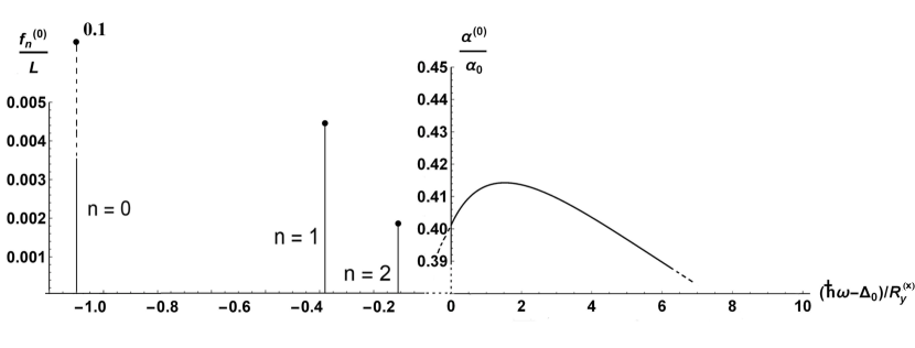
Figure 1: The specific oscillator strengths $\frac{f_{n}^{(0)}}{L}$ (eq. (46)) and continuous absorption $\frac{\alpha^{(0)}}{\alpha_{0}}$ (eq. (47)) associated with the ground $(N=0)$ energy gap $\Delta_{0}=0.69\,\mbox{eV}\,$ as a function of the frequency shift $\hbar\omega-\Delta_{0}$ scaled with the exciton Rydberg constant $Ry^{\mbox{\tiny(x)}}=13.8\,\mbox{meV}\,$ (43) in the AGNR of width $d=2\,\mbox{nm}\,$ placed on the sapphire substrate ($q\simeq 0.40$.)

All the Rydberg series $\alpha_{n}^{(N)}$, except for $\alpha_{n}^{(0)}$ adjacent to the ground size-quantized level $N=0$, overlap with the branches of the continuous spectra, originating from the lower $N$-levels. As a result only the ground series $N=0$ is formed by transitions to the strictly discrete exciton states, while the others $N\neq 0$ series are associated with transitions to the Fano resonant states, induced by the inter-subband coupling between the overlapping discrete $(n)$ and continuous $(s)$ exciton states, related to various subbands Fano . Thus in the multi-subband approximation only the ground exciton Rydberg series $\alpha_{n}^{(0)}$ (42) is composed of $\delta$-function type peaks, while the others $\alpha_{n}^{(N)},N\neq 0$ consist of the absorption maxima of finite height and nonzero Fano frequency width $\Gamma_{Nn}$, previously calculated for the impurity electron in AGNR Monschm12 and for low-dimensional semiconductor structures (see Monschm09 and references therein). Below we focus on the exciton absorption spectrum associated with the ground size-quantized subband $N=0$ (see Fig.1). The corresponding results coincide qualitatively with those calculated in the single-subband approximation for the frequency regions relevant to the subbands $N\neq 0$.

It follows from eqs. (42) and (46) that the oscillator strengths of exciton peaks of the $\delta$-function type at frequencies (43) rapidly decrease as $\sim n^{-3}$ with increasing quantum number $n$. The intensities of the excited peaks $n\geq 1$ scaled with the ground maximum $n=0$ obey the inequality $\beta_{0n}^{2}\beta_{00}/n^{3}\ll 1$. Thus as presented in Fig.1, optical absorption at $\hbar\omega<\Delta_{0}$ is practically concentrated in the region of transition to the ground exciton state $n=0$. On narrowing the ribbon, the positions of peaks (43) $\omega_{n}\sim d^{-1}$ shift towards higher frequencies, and their oscillator strengths $f_{n}^{(0)}\sim|c_{0}(n)|^{2}$ increase in magnitude (Fig.2).

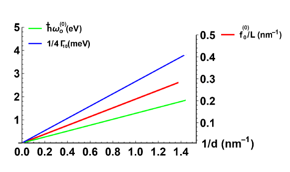
Figure 2: The ground exciton peak position $\hbar\omega_{0}^{(0)}$ (eqs. (43), (33)), its specific oscillator strength $\frac{f_{0}^{(0)}}{L}$ (46) and the resonant width $\Gamma_{10}$ (eq. (60)) versus the inverse ribbon width $d^{-1}$ of the AGNR situated on a sapphire substrate ($q\simeq 0.40$.)

With decreasing ribbon width $d$ the distance $|\hbar\omega_{n}^{(0)}-\Delta_{0}|\sim d^{-1}$ between the frequency positions of peaks $\omega_{n}^{(0)}$ and the edge of continuous absorption $\Delta_{0}/\hbar$ increases, which in turn makes the narrow AGNR preferable candidates for the experimental study of a discrete exciton spectrum. The dependencies of the binding energy of the ground exciton state $E_{00}^{(b)}=\Delta_{0}-E_{00}$ calculated from eq. (35), of the corresponding specific oscillator strength $f_{0}^{(0)}/L$ and of the width $\Gamma_{10}$ on the inverse ribbon width $d^{-1}$ and on the exciton interaction strength $q$ are shown in Fig.3.

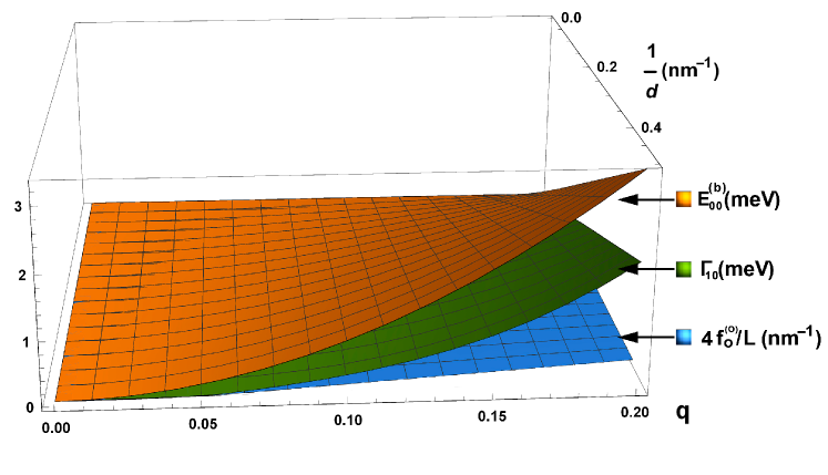
Figure 3: The dependencies of the binding energy $E_{00}^{(b)}$ (eq.(35)) of the ground discrete exciton state, of the corresponding specific oscillator strength $\frac{f_{0}^{(0)}}{L}$ (eq. (46)) and of the resonant width $\Gamma_{10}$ (eq. (60)) of the ground quasi-discrete exciton state on the inverse ribbon width $d^{-1}$ and on the dimensionless exciton parameter $q$ defined in eq. (24).

In the continuous spectral region $\hbar\omega\geq\Delta_{0}$ (Fig.1) the exciton absorption $\alpha^{(0)}(\omega)$ (47) is the fundamental absorption $\alpha^{(0)}(\omega)\sim\zeta\sim(\hbar\omega-\Delta_{0})^{-\frac{1}{2}}$ modified by the 1D Zommerfeld factor $Z(\zeta)$, taking into account the exciton attraction of the electron and hole. For the frequencies positioned far away from the edge $(\zeta\ll 1)$, the exciton interaction has little effect $(Z\simeq 1)$ on the fundamental absorption. In the vicinity of the edge $(\zeta\rightarrow\infty~{},\,Z\rightarrow(2\pi\zeta)^{-1})$ the exciton factor modifies strongly the fundamental absorption compensating the singularity $\sim\zeta$ and providing the finite absorption $\alpha^{(0)}(\omega)$ (49) at the edge and the linear addition $\Delta\alpha^{(0)}\sim\zeta^{-2}$ nearby the edge. The main characteristics of the optical spectrum, represented in Fig.1, namely the radical redistribution of the absorbed radiation in favor of the ground peak and the disappearance of the singularity of the 1D density of states, are the common signatures of the 1D exciton absorption. Earlier this was found for 1D excitons in bulk semiconductors subject to a strong magnetic field Hashow and in semiconductor quantum wires Monschm09 . Recently an analogous result was obtained by Portnoi et al. Port employing a 1D quasi-Coulomb potential for the calculation of the exciton absorption spectrum in narrow-gap carbon nanotubes.

It follows from eqs. (42) and (57) derived in the double-subband approximation that the inter-subband coupling modifies the quasi-Rydberg exciton series adjacent to the excited size-quantized energy levels $N\neq 0$, thereby replacing the $\delta$-function type optical peaks for which $\alpha_{n}^{(N)}(\omega)\sim f_{n}^{(N)}\delta(\hbar\omega-E_{Nn})$, by those of the Lorentzian form with finite maxima $\Lambda_{\mbox{max}}\sim\frac{2}{\pi\Gamma_{Nn}}$ and nonzero width $\Gamma_{Nn}$. The resonant peaks are red-shifted by an amount $\Delta E_{Nn}$. Since the resonant shifts $\Delta E_{Nn}$ and widths $\Gamma_{Nn}$ can be qualitatively described by eqs. (59) and (60), respectively, we take

$$\Gamma_{Nn}\sim E_{Nn}^{(b)}\frac{q}{\kappa_{Nn}};~{}\Delta E_{Nn}\sim-E_{Nn}^{(b)}\frac{q^{2}}{\kappa_{Nn}};~{}E_{Nn}^{(b)}\sim\Delta_{N}\frac{q^{2}}{\kappa_{Nn}^{2}};\quad\kappa_{Nn}=n+\beta_{Nn}.$$

Note firstly that the resonant shifts $\Delta E_{Nn}\sim\Delta_{N}q^{4}$ are much less than the resonant widths $\Gamma_{Nn}\sim\Delta_{N}q^{3}$ at $q\ll 1,~{}(\Delta E_{Nn}\ll\Gamma_{Nn})$ and secondly the resonant shifts do not change the discrete character of the exciton energy spectrum at $E\leq\Delta_{N}$, while the resonant widths are the characteristics of the continuous spectrum accounting for the finite life-times $\tau_{Nn}=\hbar/\Gamma_{Nn}$ of the exciton states. We point out that the relationship between $\Delta E_{Nn}$ and $\Gamma_{Nn}$ strongly depends on the dimension of the structure. For 1D structures, namely AGNR, bulk semiconductors subject to strong magnetic fields Zhilmak and quantum wires Monschm09 , $\Delta E_{Nn}\ll\Gamma_{Nn}$, while for 2D systems such as QW Monschm05 and superlattices Monschm07 , $\Delta E_{Nn}\gg\Gamma_{Nn}$. Eq. (60) and Figs. 2 and 3 show that the resonant widths $\Gamma\sim E^{(b)}q,~{}q\simeq\frac{d}{a_{\mbox{\tiny x}}(d)}$ increase with decreasing ribbon width $d$. This dependence is opposite to that in a QW, in which the narrowing of the well decreases the resonant widths $\Gamma^{(w)}\sim E_{w}^{(b)}q_{w}^{4};~{}q_{w}=\frac{d}{a_{\mbox{\tiny x}}^{(w)}}$ Monschm05 . This is because the dependencies of the binding energies $E^{(b)}$ and the adiabaticity parameter $q$ are completely different for the AGNR and QW. In the AGNR $E^{(b)}\sim\Delta_{N}\sim d^{-1}$ increases on narrowing the ribbon, while $q\sim\frac{d}{a_{\mbox{\tiny x}}(d)}$ does not depend on the ribbon width $d$. In a QW the binding energy $E_{w}^{(b)}\sim Ry_{w}^{\mbox{\tiny(x)}}\sim\frac{1}{a_{\mbox{\tiny x}}^{(w)2}}$ and the Bohr radius $a_{\mbox{\tiny x}}^{(w)}$ are independent of the well width $d$, while with decreasing $d$ the parameter $q_{w}\sim\frac{d}{a_{\mbox{\tiny x}}^{(w)}}\sim d$ decreases as well. The analogous conclusion is valid for the resonant widths of the exciton states in a semiconductor superlattice Monschm07 . Exciton peaks associated with the transitions to the excited resonant states $n=1,2,\ldots$ are much narrower than that corresponding to the ground state $n=0$ with $\Gamma_{1n}/\Gamma_{10}\simeq\beta_{1n}^{2}\beta_{10}/2n^{3}\ll 1.$ This strongly affects the relationship between the maximum values of peaks of absorption (57) at $\hbar\omega=E_{1n}+\Delta E_{1n}$

$$\alpha_{n\mbox{\tiny max}}^{(1)}=\alpha^{(0)}\frac{8p^{2}f_{n}^{(1)}}{n_{b}\Delta_{1}dL\Gamma_{1N}}$$

related to the ground $n=0$ and excited $n=1,2.\ldots$ exciton states. It follows from Eqs. (46) and (60) for the oscillator strengths and the resonant widths, respectively, that $\frac{\alpha_{n\mbox{\tiny max}}^{(1)}}{\alpha_{0\mbox{\tiny max}}^{(1)}}=1.$ Thus in contrast to the exciton series adjacent to the ground subband $N=0$ for which the ground exciton peak $n=0$ significantly exceeds in intensity the excited ones $n=1,2,\ldots$ $\left(\frac{f_{n}^{(0)}}{f_{0}^{(0)}}=\frac{\beta_{0n}^{2}\beta_{00}}{2n^{3}}\ll 1\right)$ the series related to the excited subbands $N\neq 0$ consist of exciton peaks with comparable intensities.

In view of possible future experiments, we estimate the edges of the inter-subband optical absorption $\hbar\omega^{(N)}=\Delta_{N}$, the exciton binding energies $E_{Nn}^{(\mbox{b})}=Ry^{\mbox{\tiny(x)}}/(n+\beta_{Nn})^{2}$ and the specific oscillator strengths $f_{n}^{(N)}/L$ of the transitions to the exciton states for the AGNR placed on a sapphire substrate $(\varepsilon\simeq 10,q\simeq 0.40)$. The latter is preferable compared to a $\mbox{SiO}_{2}$ substrate $(\varepsilon\simeq 3.9)$, which provides a smaller screening of the electron-hole attraction and larger value of the parameter $q$. The energy gaps, the binding energies and the oscillator strengths determine the exciton peak positions (43) and their intensities (46), respectively. The edges of optical absorption calculated from eq. (15) $\Delta_{N}=2\varepsilon_{N}$ for $N=0,1,-1,2,-2,3~{};\tilde{\sigma}=\frac{1}{3}$ for the ribbon consisting of 55 dimers $(d\simeq 6.6~{}\mbox{nm})$ and those presented by Sasaki et al. (Fig.3 in Ref. Sas ) are given in Table 1. For the ribbon of width $d\simeq 1.7~{}\mbox{nm}$ (15 dimers) eq. (15) and Sasaki et al. calculations lead to amounts $\Delta_{0}\simeq 0.80~{}\mbox{eV~{}\,and}\quad\Delta_{0}^{*}\simeq 0.66~{}\mbox{eV}$, respectively.

$N$	$0$	$1$	$-1$	$2$	$-2$	$3$
$\Delta_{N}$	0.20	0.40	0.80	1.0	1.4	1.6
$\Delta_{N}^{*}$	0.20	0.40	0.80	0.9	1.4	1.5

Table 1: The edges of the optical absorption calculated from eq. (15) $\Delta_{N}=2\varepsilon_{N}$ for $N=0,1,-1,2,-2,3~{};\tilde{\sigma}=\frac{1}{3}$ and those $\Delta_{N}^{*}$ given in Ref. Sas .

Son et al. Son calculated the energy gap $\Delta_{0}^{*}=0.50~{}\mbox{eV}$ for the ribbon of width $2~{}\mbox{nm}$ with hydrogen passivated edges. On excluding the $12\%$ gap reduction caused by the passivation resulting in $\Delta_{0}^{*}=0.57~{}\mbox{eV}$ we compare the later with our optical edge found from eq. (15) $\Delta_{0}=0.69~{}\mbox{eV}$. As expected, our data for $\Delta_{N}$ and the values of $\Delta_{0}^{*}$ presented in Refs. Sas and Son are in very good agreement (see Table 1) for a relatively wide ribbon $(d\geq 6~{}\mbox{nm})$, but not for narrow samples $(d\leq 2~{}\mbox{nm})$. The reason therefore is that the analytical Dirac equation method treating the ribbon as a continuous medium is good for wide ribbons, while the numerical tight-binding approximation, which takes into account the discrete atomic structure of a ribbon, provides more accurate results for narrow samples. The calculation of the binding energy $E_{00}^{(\mbox{b})}$ of the ground exciton state $(n=0)$ located within the ground energy gap $(N=0)$ using eqs. (43), (35) and (33) for an AGNR of width $d=1~{}\mbox{nm}$ placed on a sapphire substrate yields a value $E_{00}^{(\mbox{b})}\simeq 30~{}\mbox{meV}$. The value of the specific oscillator strength $\frac{f_{0}^{(0)}}{L}\simeq\frac{q}{2\beta_{00}d}$ calculated using eqs. (46) and (33) is equal to $\frac{f_{0}^{(0)}}{L}\simeq 0.20~{}\mbox{nm}^{-1}$. The relatively small values of the binding energy and specific oscillator strength are the consequences of high dielectric constant $\varepsilon$ of the substrate, which ensures the condition $q<<1$ for the adiabatic approximation. Any detailed quantitative comparison of our results with those obtained earlier by both analytical and numerical methods is problematic because the latter were obtained under different conditions, e.g., for a suspended AGNR $(q=2.2)$ Zhu ; Jia and hydrogen-passivated edges Prez or with an unspecified dielectric constant $\epsilon_{\mbox{\tiny eff}}(\vec{r})$ Mohamm .

We estimate the binding energy $E_{10}^{(\mbox{b})}=\Delta_{1}-\hbar\omega_{0}^{(1)}$ of the ground Fano-resonant exciton state $n=0,N=1$, using eq. (43) for an AGNR of width $d=2~{}\mbox{nm}$ placed on the sapphire substrate. The quantum defect $\beta_{10}$ determining the binding energy $E_{10}^{(\mbox{b})}$ has been calculated from eqs. (32) and (33). For the strictly discrete ground series $N=0$ of the considered AGNR, $E_{00}^{(\mbox{b})}=15~{}\mbox{meV}$, which exceeds the binding energy $E_{10}^{(\mbox{b})}\simeq 3.8~{}\mbox{meV}$. The latter is in line with the conclusion made in Ref. Zhilmon that the exciton series relevant to the $N$-subband become markedly suppressed with increasing subband index $N$.

The width $\Gamma_{10}$ (60) and the maximum absorption coefficient $\alpha_{0\mbox{\tiny max}}^{(1)}$ (57) with $n_{b}\simeq 1.8$ possess the values $\Gamma_{10}\simeq 5.75~{}\mbox{meV}~{}\mbox{and}~{}\alpha_{0\mbox{\tiny max}}^{(1)}=0.214$. Clearly, the exciton Fano resonances with the lifetimes $\tau=\hbar/\Gamma_{10}=0.12~{}\mbox{ps}$ can be detected in optical experiments with narrow AGNR. The considerable enhancement of exciton optical absorption in quasi-1D AGNR with respect to excitonless 2D graphene layers, for which $\alpha_{0}=2.3\cdot 10^{-2}$ can be used in optoelectronics and applied optics. We believe that the proposed analytical approach will be useful for both theoretical studies and practical applications of the scalable exciton effects in the AGNR.

VII Conclusions

We have developed an analytical approach to the problem of the exciton absorption in the narrow gap armchair graphene nanoribbon. The ribbon width is taken to be much less than the exciton Bohr radius. This adiabatic criterion allows us to solve analytically the two-body 2D Dirac equation, describing the interacting massless electron-hole pair and then to calculate the optical absorption coefficient in an explicit form. With the coupling between the different subbands taken into account, the Fano resonances appear instead of strictly discrete exciton states. The exciton spectrum is a sequence of Rydberg series of strictly discrete or broadened resonant peaks positioned within the gaps determined by the electron-hole size-quantized energy levels and continuous bands, branching from the tops of the gaps. The intensities, frequency widths, and blue shifts of exciton peaks increase on narrowing the ribbon. At the edges, the exciton effect eliminates the singularities in the fundamental absorption. Our analytical results are in good agreement with those obtained by using other theoretical approaches, in particular, with the results of numerical studies. The expected experimental values are estimated for concrete AGNR.

VIII Acknowledgments

The authors are grateful to D. Turchinovich and V. Bulychev for useful discussions and to T. Fedorova for technical assistance.

References

- (1) K. Wakabayashi, K. Sasaki, T. Nakanishi, Sci. Technol. Adv. Mater. 11, 054504 (2010)
- (2) J. Alfonsi and M. Meneghetti, New J. Phys. 14, 053047 (2012)
- (3) G. Soavi, S. D. Conte, C. Manzoni, D. Viola, A. Narita, Y. Hu, X. Feng, U. Hohenester, E. Molinari, D. Prezzi, K. Müllen and G. Cerullo, Nat. Commun. 7, 11010 (2016)
- (4) H. Hasegawa and R.E. Howard, J. Phys. Chem. Solids 21, 179 (1961)
- (5) B. S. Monozon and P. Schmelcher, Phys. Rev. B 79, 165314 (2009)
- (6) D. S. Novikov, Phys. Rev. B 76, 245435 (2007)
- (7) B. S. Monozon and P Schmelcher, Phys. Rev. B 86, 245404 (2012)
- (8) B. S. Monozon and P Schmelcher, Phys. Rev. B 71, 085302 (2005)
- (9) L. Yang, M. Cohen and S. Louie, Nano Lett. 7, 3112 (2007)
- (10) D. Prezzi, D. Varsano, A. Ruini, A. Marini and E. Molinari, Phys. Rev. B 77, 041404(R) (2009)
- (11) X. Zhu and H. Su, J. Phys. Chem. A 115, 11998 (2011)
- (12) R. Denk, M. Hohage, P. Zeppenfeld, J. Cai, C. A. Pignedoli, H. Sode, R. Fasel, X. Feng, K. Mullen, S. Wang, D. Prezzi, A. Ferretti, A. Ruini, E. Molinari and P. Ruffieux Nature Communications 5, 4253 (2014)
- (13) Y. L. Jia, X. Geng, H. Sun and Y. Luo, Eur. Phys. J. B 83, 451 (2011)
- (14) Y. Lu, S. Zhao, W. Lu, H. Liu and W. Liang, J. Appl. Phys. 115, 103701 (2014)
- (15) P. V. Ratnikov and A. P. Silin, JETP 114, 512 (2012)
- (16) L. Mohammadzadeh, A. Asgari, S. Shojaei and E. Ahmadi, Eur. Phys. J. B 84, 249 (2011)
- (17) U. Fano, Phys. Rev. B 124, 1866 (1961)
- (18) B. S. Monozon and P Schmelcher, Phys. Rev. B 90, 125313 (2014)
- (19) H. Hsu and L. E. Reichl, Phys. Rev. B 76, 045418 (2007)
- (20) K. Gundra and A. Shukla, Phys. Rev. B 83, 075413 (2011)
- (21) Ken-ichi Sasaki, K. Kato, Y. Tokura, K. Oguri and T. Sogawa, Phys. Rev. B 84, 085458 (2011)
- (22) R. J. Elliot, Phys. Rev. B 108, 1384 (1957)
- (23) M. M. Mahmoodian and M. V. Entin, Nanoscale Res. Lett. 7, 599 (2012)
- (24) L. Brey and H. A. Fertig, Phys. Rev. B 73, 235411 (2006)
- (25) E. H. Hwang and S.Das Sarma, Phys. Rev. B 75, 205418 (2007)
- (26) A. H. Castro Neto, F. Guinea, N. M. R. Peres, K. S. Novoselov, and A. K. Geim, Rev. Mod. Phys. 81, 109 (2009)
- (27) Handbook of Mathematical Functions, edited by M. Abramowitz and I. A. Stegun (Dover, New York, 1972)
- (28) Y.-W. Son, M. L. Cohen and S. G. Louie, Phys. Rev. Lett. 97, 216803 (2006)
- (29) M. E. Portnoi, C. A. Downing, R. R. Hartmann, and I. A. Shelykh, 15th International Conference on Electromagnetics in Advanced Applications (ICEAA’13), Turin, Italy, September 9-13, 2013, IEEE Catalogue Number: CFP1368B-CDR, pp. 231-234
- (30) A. G. Zhilich and O. A. Maksimov, Sov. Phys. Semicond. 15, 1108 (1981)
- (31) B. S. Monozon and P Schmelcher, Phys. Rev. B 75, 245207 (2007)
- (32) A. G. Zhilich and B. S. Monozon, Sov. Phys. Solid State. 8, 2846 (1967)