Semiclassical theory of the magnetization process of the triangular lattice Heisenberg model

Abstract

Motivated by the numerous examples of 1/3 magnetization plateaux in the triangular lattice Heisenberg antiferromagnet with spins ranging from 1/2 to 5/2, we revisit the semiclassical calculation of the magnetization curve of that model, with the aim of coming up with a simple method that allows one to calculate the full magnetization curve, and not just the critical fields of the 1/3 plateau. We show that it is actually possible to calculate the magnetization curve including the first quantum corrections and the appearance of the 1/3 plateau entirely within linear spin-wave theory, with predictions for the critical fields that agree to order 1/S with those derived a long-time ago on the basis of arguments that required to go beyond linear spin-wave theory. This calculation relies on the central observation that there is a kink in the semiclassical energy at the field where the classical ground state is the collinear up-up-down structure, and that this kink gives rise to a locally linear behavior of the energy with the field when all semiclassical ground states are compared to each other for all fields. The magnetization curves calculated in this way for spin 1/2, 1 and 5/2 are shown to be in good agreement with available experimental data.

I Introduction

In strongly correlated electron systems quantum fluctuations are responsible for the manifestation of a variety of exotic behaviors. In the field of magnetic insulators, for instance, their effect can range from the stabilization of magnetic order to the emergence of non magnetic spin liquid phasesLacroix et al. (2011). Of recent theoretical and experimental interest are the properties of frustrated magnetic insulators in external magnetic fields. In these systems, quantum fluctuations, which are enhanced by frustration, may lead to the presence of anomalies of the magnetization curve. Of specific relevance to our study are magnetization plateaus. These consist of a constant magnetization at a rational value of the saturation which persists over a finite field interval. While plateau states break the translational symmetry of the lattice, the nature of the plateau wavefunction greatly depends on the details of the model. Examples include crystals of purely quantum objects such as triplet excitations in ladder systemsTotsuka (1998); Mila (1998), crystals of more involved objects such as bound states of triplets as in the Shastry Sutherland lattice Corboz and Mila (2014) or valence bond crystals as identified for the $S=1/2$ Heisenberg antiferromagnet on the kagome lattice Cabra et al. (2005); Capponi et al. (2013); Nishimoto et al. (2013). Such plateaux are usually referred to as ’quantum’ plateaux because the state which is stabilized has no classical analog.

By contrast, there are plateaux for which the magnetization pattern has a simple classical analog consisting of a crystal of down pointing spins in a background of spins aligned with the magnetic field Kawamura (1984); Chubukov and Golosov (1991); Zhitomirsky et al. (2000); Penc et al. (2004); Coletta et al. (2013). Such plateaux are sometimes referred to as ’classical’ plateaux. Given the essentially classical nature of such plateaux, it seems logical to expect that a purely semiclassical theory can be developed, and indeed the first prediction of a 1/3 plateau in the triangular lattice Heisenberg antiferromagnet by Chubukov and Golosov was based on semiclassical argumentsChubukov and Golosov (1991). They showed, going beyond linear spin wave theory, that the $1/3$ plateau state with a $3$-sublattice up-up-down structure acquires a spin gap in a finite field range, and that the critical fields at which the gap closes correspond to those at which the structure stops being collinear. Since the seminal work of Chubukov et al. the existence of the $1/3$ plateau was confirmed numerically by exact diagonalizations of finite size clusters for spin $S=1/2$ Honecker et al. (2004) and $S=1$ Shirata et al. (2011); Richter et al. (2013), as well as by the coupled cluster expansion Farnell et al. (2009). Moreover several experimental realizations have been discovered: the compound Cs₂CuBr₄, though with an orthorhombic distortion Ono et al. (2003, 2004); Tsujii et al. (2007); Fortune et al. (2009), and the much closer realization of an ideal triangular lattice antiferromagnet Ba₃CoSb₂O₉ Shirata et al. (2012); Susuki et al. (2013). Both these compounds are relevant for the spin $S=1/2$ case. Additionally we note that the compounds Ba₃NiSb₂O₉ and RbFe(MoO₄)₂ are other realizations of the same model but this time the on-site magnetic moment is respectively a spin $S=1$ Shirata et al. (2011); Richter et al. (2013) and a spin $S=5/2$ Svistov et al. (2003, 2006); Smirnov et al. (2007); Kenzelmann et al. (2007); White et al. (2013). In all of these systems magnetization measurements report the existence of a $1/3$ plateau.

Actually, Chubukov and Golosov did not calculate the magnetization curve outside the $1/3$ plateau using a semiclassical approach. Such a calculation has been achieved years later in the case of the square lattice antiferromagnet by Zhitomirsky and NikuniZhitomirsky and Nikuni (1998), who showed that a semiclassical calculation of the magnetization curve is actually possible without going beyond the linear approximation if the magnetization is extracted from the derivative of the energy with respect to the field. The goal of the present paper is to show how this calculation can be extended to the case of the triangular lattice. This enterprise, which at first sight looks like a simple exercise, turned out to be far more subtle than expected, and to raise a number of interesting questions. As we shall see, the magnetization curve calculated along the lines of Zhitomirsky and Nikuni is unphysical around the field where the classical ground state is the up-up-down state with magnetization 1/3, and curing this unphysical behavior leads to an alternative semiclassical theory of the 1/3 magnetization plateau entirely based on energy considerations which do not require to go beyond linear order. The main conclusion is that it is indeed possible to calculate the magnetization curve of the triangular lattice Heisenberg AFM including the 1/3 plateau within linear spin-wave theory. Remarkably enough, the critical fields derived by this alternative approach turn out to have the same value as those predicted by Chubukov and Golosov, whose approach required to go beyond linear spin-wave theory.

To achieve this we will start by reminding the classical solution of the model (Sec. II) and the linear spin wave prediction for the magnetization (Sec. III). Then we will discuss a phenomenological theory (Sec. IV) which we will then put on a more microscopic basis in the context of a variational arguments (Sec. V). After comparing the results with available experiments (Sec. VI), we will conclude with a discussion of the validity and usefulness of the present results.

II Classical Solution

The Hamiltonian of the triangular lattice Heisenberg antiferromagnet in a magnetic field is given by

$$\mathcal{H}=\frac{J}{S^{2}}\sum_{\langle i,j\rangle}{\bf S}_{i}\cdot\ {\bf S}_{j}-\frac{H}{S}\sum_{i}S_{i}^{z}\,,$$ (1)

where the first sum is taken over all nearest neighbors of the triangular lattice [see Fig. 1 a)].

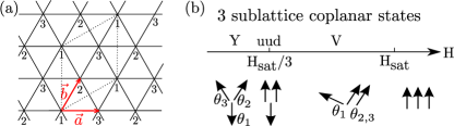
Figure 1: a) Triangular lattice and $3-$sublattice structure. The numbering indicates equivalent lattice sites. b) Sketch of the $3-$sublattice Y and V coplanar structures at different field values.

Up to a constant the Hamiltonian (1) can be rewritten as a sum over all triangular plaquettes of the lattice as

$$\mathcal{H}=\sum_{p}\frac{J}{4S^{2}}\left({\bf S}_{p,1}+{\bf S}_{p,2}+{\bf S}_{p,3}-\frac{{\bf H}S}{3J}\right)^{2}\,,$$ (2)

with subscripts $1,2,3$ denoting the three spins belonging to the plaquette $p$. At the classical level, when the spin operators are replaced by three dimensional vectors of norm $S$, Eq. (2) indicates that the energy of the system is minimal when on all triangles of the lattice the total spin fulfills the constraint $({\bf S}_{p,1}+{\bf S}_{p,2}+{\bf S}_{p,3})=(S/3J){\bf H}$. The resulting classical ground state manifold is accidentally degenerate. For instance, both coplanar and umbrella like configurations minimize the classical energy. Chubukov and Golosov showed that this accidental degeneracy is lifted at $T=0$ by quantum fluctuations in favor of the coplanar states Chubukov and Golosov (1991). The $3-$sublattice coplanar states stabilized in the linear spin wave approximation can be parametrized by three angles measured with respect to the field direction [see Fig. 1 b)]. They are the Y state parametrized by $(\theta_{1}^{Y},\theta_{2}^{Y},\theta_{3}^{Y})$ with $\theta_{1}^{Y}=\pi$ and $\theta_{2}^{Y}=-\theta_{3}^{Y}=\textrm{acos}{[\left(3J+H\right)/6J]}$ for $0\leq H\leq 3J$ and the V state parametrized by $(\theta_{1}^{V},\theta_{2}^{V},\theta_{3}^{V})$ with $\theta_{1}^{V}=-\textrm{acos}{[(-27J^{2}+H^{2})/6HJ]}$ and $\theta_{2}^{V}=\theta_{3}^{V}=\textrm{acos}{[(27J^{2}+H^{2})/12HJ]}$ for $3J\leq H\leq 9J$. When the field is at $1/3$ of the saturation value the Y and V states are identical to the uud structure with two spins pointing along the field and one pointing down on each triangular plaquette of the lattice.

In the next section we present some basic results of the spin wave approximation for the Y and V coplanar structures.

III Linear-spin wave approximation

III.1 General formalism

The spin wave approximation consists in the bosonic reformulation of the quantum spin problem in terms of Holstein-Primakoff (HP) particles which represent deviations from the underlying classical order and assuming these deviations to be small compared to the size of the classical moments. This approach is formalized in two steps: first the quantum spin Hamiltonian is rewritten by expressing the spin operators in the local basis of the classical spin orientations denoted $(x^{\prime},y^{\prime},z^{\prime})$. Supposing that the coplanar Y and V structures lie in the $xz$ plane, this can be done as follows

$$\begin{array}[]{l}S_{{\bf R},i}^{x}=\cos\theta_{i}S_{{\bf R},i}^{x^{\prime}}+\sin\theta_{i}S_{{\bf R},i}^{z^{\prime}}\,,\\ S_{{\bf R},i}^{y}=S_{{\bf R},i}^{y^{\prime}}\,,\\ S_{{\bf R},i}^{z}=\cos\theta_{i}S_{{\bf R},i}^{z^{\prime}}-\sin\theta_{i}S_{{\bf R},i}^{x^{\prime}}\end{array}$$ (3)

where the angles $\theta_{i}$ parametrize the Y and V states, ${\bf R}$ is a vector of the super lattice and $i=1,2,3$ denotes the sublattice [see Fig. 1 a)]. In this rotated frame, the classical ground state is ferromagnetic by construction.

Secondly, deviations from the classical order are expressed in terms of the Holstein-PrimakoffHolstein and Primakoff (1940) representation of spin operators. To next to leading order the expressions take the form

$$\begin{array}[]{lll}S_{{\bf R},i}^{x^{\prime}}&=&\displaystyle\frac{\sqrt{2S}}{2}(a_{{\bf R},i}^{\phantom{\dagger}}+a_{{\bf R},i}^{\dagger})-\frac{1}{4\sqrt{2S}}\left(n_{{\bf R},i}^{\phantom{\dagger}}a_{{\bf R},i}^{\phantom{\dagger}}+a_{{\bf R},i}^{\dagger}n_{{\bf R},i}^{\phantom{\dagger}}\right)+\ldots\\[8.53581pt] S_{{\bf R},i}^{y^{\prime}}&=&\displaystyle\frac{\sqrt{2S}}{2i}(a_{{\bf R},i}^{\phantom{\dagger}}-a_{{\bf R},i}^{\dagger})-\frac{1}{4i\sqrt{2S}}\left(n_{{\bf R},i}^{\phantom{\dagger}}a_{{\bf R},i}^{\phantom{\dagger}}-a_{{\bf R},i}^{\dagger}n_{{\bf R},i}^{\phantom{\dagger}}\right)+\ldots\\[8.53581pt] S_{{\bf R},i}^{z^{\prime}}&=&S-n_{{\bf R},i}^{\phantom{\dagger}}\,.\\ \end{array}$$ (4)

This transformation allows to rewrite the quantum Hamiltonian (1) as a sum

$$\mathcal{H}=\sum_{n=0}^{\infty}\mathcal{H}^{(n)}\,,$$ (5)

where $\mathcal{H}^{(n)}\propto S^{-n/2}$ contains only products of $n$ bosonic operators. The first term of this series, $\mathcal{H}^{(0)}$, is the classical energy of the state around which fluctuations are considered. By construction, $\mathcal{H}^{(1)}$ vanishes identically since we expand around the 3-sublattice coplanar spin configurations which are minima of the classical energy. $\mathcal{H}^{(2)}$ describes the single particle dynamics and all higher order terms in the expansion consist of many particle interaction processes. Note that the bosonic representation is an exact mapping of the original quantum model. The spin wave approximation consists of a truncation scheme based on an expansion in powers of $1/S$, the inverse of the magnetic moment being the small expansion parameter.

III.2 Ground state energy in the harmonic approximation

At the harmonic approximation, which consists in truncating the expansion (5) to $n\leq 2$, the Fourier space expression of the fluctuation Hamiltonian is given by

$$\mathcal{H}^{(0)}+\mathcal{H}^{(1)}+\mathcal{H}^{(2)}=NE_{\textrm{cl}}+\frac{1}{2S}\sum_{\bf k}\Bigl{[}{\bf a}_{\bf k}^{\dagger}M_{\bf k}^{\phantom{\dagger}}(H){\bf a}_{\bf k}^{\phantom{\dagger}}-\Delta_{\bf k}\Bigr{]}\ ,$$ (6)

where $E_{\textrm{cl}}=-3J/2-H^{2}/18J$ is the classical energy per site of the 3-sublattice coplanar states and $N$ the number of lattice sites. Since the states considered have $3$ sites per unit cell, three distinct bosonic fields need to be introduced and thus the term ${\bf a}_{\bf k}^{\dagger}$ in Eq. (6) denotes the vector $(a_{{\bf k},1}^{\dagger},a_{{\bf k},2}^{\dagger},a_{{\bf k},3}^{\dagger},a_{{-\bf k},1}^{\phantom{\dagger}},a_{{-\bf k},2}^{\phantom{\dagger}},a_{{-\bf k},3}^{\phantom{\dagger}})$. $M_{\bf k}$ is a $6\times 6$ matrix whose structure is detailed in the Appendix A. The $1/S$ corrections to the classical energy are obtained by diagonalizing the fluctuation Hamiltonian (6) via a Bogolyubov transformation. The diagonal representation of (6) consists of a sum over $3$ independent modes of free bosonic quasiparticles.

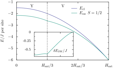
Figure 2: (Color online) Energy per site corrected by harmonic fluctuations for the coplanar Y and V type structures (green) and classical energy (blue). Inset: harmonic corrections to the classical energy. A ”kink” is visible in the energy corrected by harmonic fluctuations at the field $H_{\textrm{sat}}/3$.

The ground state energy per site corrected by fluctuations at $S=1/2$ is depicted in Fig. 2. As can be seen in the figure, the energy presents a ”kink” [discontinuity in the first derivative] at $H=H_{\textrm{sat}}/3$, the value of the field at which the classical ground state is the uud state, as first noticed by Nikuni and Shiba [Nikuni and Shiba, 1993]. This cusp, present for all values of the expansion parameter $1/S$, is most pronounced for $S=1/2$. Quantum fluctuations are responsible for the emergence of the kink in the energy, whereas the classical energy is differentiable (see blue curve in Fig. 2).

III.3 Magnetization curve

According to the Hellmann-Feynman theorem Hellmann (1937); Feynman (1939), the zero temperature expression of the average magnetization per site is given by

$$m=-\frac{1}{N}\frac{\partial E_{0}}{\partial H}\,,$$ (7)

where $N$ denotes the number of lattice sites and $E_{0}$ is the ground state energy. To first order in $1/S$ the magnetization can be obtained from the derivative with respect to the field of the energy corrected by the zero point motionZhitomirsky and Nikuni (1998) $E_{0}^{\textrm{harm}}$ according to

$$m=-\frac{1}{N}\frac{\partial E_{0}^{\textrm{harm}}}{\partial H}\,.$$ (8)

The average magnetization is presented in Figure 3 for $S=1/2$. When the $1/S$ corrections are included, the magnetization deviates from the straight line classical behavior. As a consequence of the kink in the spin wave energy as a function of the field, the magnetization displays a discontinuity at $H=H_{\textrm{sat}}/3$. Associated to the discontinuity there is a ”negative jump” in the magnetization occurring as the field is increased above $H_{\textrm{sat}}/3$. This non monotonous behavior of the magnetization is of course unphysical and must be an artifact of the harmonic truncation of the $1/S$ expansion.

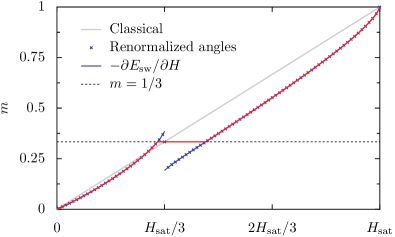
Figure 3: (Color online) Plots of the classical magnetization (black solid line) and of the magnetization including corrections to first order in $1/S$ for $S=1/2$ (blue curve). The $1/S$ corrections to the magnetization are computed in two equivalent ways: either as the derivative of the energy with respect to the magnetic field (blue curve) or by direct calculation taking into account the renormalization of the spin orientations (crosses). The overall $1/S$ magnetization curve obtained from our phenomenological approach is shown in red.

IV Phenomenological theory of magnetization

Since it is known from the work of Chubukov and Golosov that there is a plateau at 1/3, a phenomenological way to correct this unphysical aspect of the semiclassical magnetization of Fig. 3 consists in cutting the magnetization curve horizontally at the value $m=1/3$. This phenomenological approach will be put on a more systematic basis in the next section. For the moment, let us prove that it leads to the same critical fields as Chubukov and Golosov.

In this phenomenological approach, the critical fields are defined by the intersection between the magnetization curve and the line $m=1/3$. In order to extract the expressions for these critical fields one requires an analytic expression for the magnetization. An expression for the magnetization can be extracted from Eq. (8). This calculation, which turns out to be more technical in the case of states with multiple sites per unit cell for which the explicit expression of the Bogolyubov transformation is not known, is presented in the Appendix A.

Alternatively, an analytic expression of the magnetization can be obtained by computing the quantum renormalization of the spin orientations following the procedure of Refs. [Jacobs et al., 1993] and [Zhitomirsky and Nikuni, 1998]. In Appendix A it is shown that this method and the one presented in the previous paragraph yield rigorously the same results for the magnetization. For non collinear states the angle renormalization procedure amounts to decoupling the cubic boson term, $\mathcal{H}^{(3)}$, of the spin wave expansion which yields an effective linear boson contribution denoted $\mathcal{H}^{(3)}_{\textrm{eff}}$. The cancellation of the overall linear boson term $\mathcal{H}^{(1)}+\mathcal{H}^{(3)}_{\textrm{eff}}$ corresponds to a new stability condition which is fulfilled by a new set of renormalized angles. The renormalized spin orientations, $\tilde{\theta_{i}}$, are expressed for each sublattice $i$ as $\cos\tilde{\theta_{i}}=\cos{\theta_{i}}+c_{i}/S$ with the coefficients $c_{i}$ given by

$$\begin{array}[]{l}\displaystyle c_{1}^{Y}=0\,,\\ \displaystyle c_{2,3}^{Y}=\cos\theta_{2}^{Y}(n_{2}-m_{23}-\Delta_{23})+\frac{1}{2}(-n_{1}+m_{21}+\Delta_{21})\,,\end{array}$$ (9)

for the Y state and by

$$\begin{array}[]{l}\displaystyle c_{1}^{V}=-2\cos\theta_{2}^{V}(m_{21}+\Delta_{21})+\cos\theta_{1}^{V}n_{1}-\frac{3J}{H}(n_{1}-4n_{2})\,,\\[8.53581pt] \displaystyle c_{2,3}^{V}=-\frac{1}{2}\cos\theta_{1}^{V}(m_{21}+\Delta_{21})+\cos\theta_{2}^{V}n_{2}+\frac{3J}{2H}(n_{1}-4n_{2})\,,\end{array}$$ (10)

for the V state, where in the above expressions we have introduced the following two body averages computed in the harmonic ground state

$$n_{i}=\langle a_{{\bf R},i}^{\dagger}a_{{\bf R},i}^{\phantom{\dagger}}\rangle\,,\quad m_{ij}=\langle a_{{\bf R},i}^{\dagger}a_{{\bf R^{\prime}},j}^{\phantom{\dagger}}\rangle\,,\quad\Delta_{ij}=\langle a_{{\bf R},i}^{\phantom{\dagger}}a_{{\bf R^{\prime}},j}^{\phantom{\dagger}}\rangle\,,$$ (11)

with the sites $({\bf R},i)$ and $({\bf R^{\prime}},j)$ being nearest neighbors.

The expression of the magnetization per site in terms of the renormalized angles is

$$m^{\textrm{Y,V}}=\frac{1}{3S}\sum_{i=1}^{3}\cos{\tilde{\theta_{i}}^{\textrm{Y,V}}}(S-n_{i})\,.$$ (12)

Collecting all terms up to order $1/S$ in (12) yields

$$\begin{array}[]{l}\displaystyle m^{Y}=\frac{H}{9J}+\frac{1}{3S}\left(-2\cos\theta_{2}^{Y}(m_{23}+\Delta_{23})+m_{21}+\Delta_{21}\right)\,,\\[8.53581pt] \displaystyle m^{V}=\frac{H}{9J}\left(1-\frac{1}{S}(\Delta_{21}+m_{21})\right)\,.\end{array}$$ (13)

This expression of the magnetization is a function of the average quantities $n_{i},m_{ij}$ and $\Delta_{ij}$ whose field dependence is presented in the Appendix A. The magnetization (13) is reported in figure 3 and coincides with that obtained from Eq. (8).

Now, Chubukov and GolosovChubukov and Golosov (1991) showed that, to leading order in $1/S$, the fields at which the Y and V structures become collinear [i.e. that is when the renormalized spin orientations, measured from the field direction, tend to $(\theta_{1},\theta_{2},\theta_{3})=(\pi,0,0)$] correspond to the critical fields at which the gaps of the renormalized spectra of the uud state vanish [see Appendix A for more details]. Below we show that the critical fields obtained by cutting the $1/S$ magnetization curve at the value $1/3$ are the same as those predicted by Chubukov and Golosov. For this purpose, let us introduce the quantities $H_{c1}=3J+\alpha/S$ and $H_{c2}=3J+\beta/S$ defined such that $m^{Y}(H_{c1})=m^{V}(H_{c2})=1/3$. Evaluating the magnetization of the Y and V states respectively at $H_{c1}$ and $H_{c2}$ and expanding in powers of $1/S$ gives, to lowest order,

$$\begin{array}[]{l}\displaystyle m^{Y}(H_{c1})=\frac{1}{3}+\frac{\alpha}{9JS}+\frac{1}{3S}\left(-2(\bar{m}_{23}+\bar{\Delta}_{23})+\bar{m}_{21}+\bar{\Delta}_{21}\right)\,,\\[8.53581pt] \displaystyle m^{V}(H_{c2})=\frac{1}{3}+\frac{\beta}{9JS}-\frac{1}{3S}(\bar{\Delta}_{21}+\bar{m}_{21})\,,\end{array}$$ (14)

where the superscript bar denotes averages that are computed at $H=H_{\textrm{sat}}/3$. Imposing $m^{Y}(H_{c1})=m^{V}(H_{c2})=1/3$ and solving for $\alpha$ and $\beta$ we obtain

$$\begin{array}[]{l}\displaystyle H_{\textrm{c1}}=3J\left(1+\frac{2\bar{m}_{23}-\bar{\Delta}_{21}}{S}\right)=3J\left(1-\frac{0.084}{S}\right)\,,\\[8.53581pt] \displaystyle H_{\textrm{c2}}=3J\left(1+\frac{\bar{\Delta}_{21}}{S}\right)=3J\left(1+\frac{0.215}{S}\right)\,,\end{array}$$ (15)

which correspond exactly to the same $1/S$ behaviors of the critical fields predicted by Chubukov and GolosovChubukov and Golosov (1991) (note that $\bar{m}_{21}=\bar{\Delta}_{23}=0$ see Appendix A).

So we have shown that this very simple approach to determine the plateau boundaries, which consists of cutting the average magnetization to the value $1/3$, produces consistent results in the large $S$ limit. In the next section we present the formal justification of why the magnetization curve should be cut precisely at the value $m=1/3$ as well as a novel perspective on the stabilization of the $1/3$ plateau which is based on the energetic comparison of the uud state with the other coplanar states.

V Variational theory of magnetization

To show that cutting the magnetization at 1/3 is the right way to correct the unphysical behavior of the semiclassical magnetization of Fig. 3, let us first show that the existence of the kink in the energy curve corrected by harmonic fluctuations implies that the uud state will be stabilized over a finite field range. Our argument is the following: in the quantum Hamiltonian of the system (1) the total spin projection in the direction of the field is a conserved quantity. Hence the energies of the eigenstates of (1) depend linearly on the field. Now, the $1/S$ expansion of the Hamiltonian around the uud structure preserves this property even if the expansion is truncated at harmonic order. In the language of Holstein-Primakoff bosons this translates into the fact that $\sum_{\bf R}\left(-n_{{\bf R},1}+n_{{\bf R},2}+n_{{\bf R},3}\right)$ commutes with the quadratic fluctuation Hamiltonian (where $1$ denotes the sublattice site with spin down and $2$ and $3$ the sublattice sites with spin up). Therefore it is possible to determine the energy of the uud state, which can be computed to order $1/S$ only at $H=H_{\textrm{sat}}/3$, at other values of the field according to

$$E_{SW}^{\textrm{uud}}(H)=E_{SW}^{\textrm{uud}}(H_{\textrm{sat}}/3)-\frac{1}{3}\left(H-\frac{H_{\textrm{sat}}}{3}\right)\,,$$ (16)

where $E_{SW}^{\textrm{uud}}(H_{\textrm{sat}}/3)$ is the energy per site of the uud state corrected by the zero point fluctuations at $H=H_{\textrm{sat}}/3$ and $1/3$ is the average magnetization per site of the uud state.

The fact that the magnetization is strictly equal to 1/3 in the uud state even when quantum fluctuations are included, as anticipated in Ref. [Chubukov and Golosov, 1991], is not completely trivial since the local magnetizations are no longer equal to $\pm 1/2$, but are renormalized by quantum fluctuations. That this is true to order $1/S$ can be explicitly verified by calculating the local magnetizations at the harmonic order, which indeed satisfy $\langle-n_{{\bf R},1}+n_{{\bf R},2}+n_{{\bf R},3}\rangle=0$. The proof that this is true to all orders is actually even simpler. Indeed, the full quantum Hamiltonian (1) can be split into the sum of two parts $\mathcal{H}^{z}=J\sum_{\langle i,j\rangle}S_{i}^{z}S_{j}^{z}-H\sum_{i}S_{i}^{z}$ and $\mathcal{H}^{xy}=J\sum_{\langle i,j\rangle}S_{i}^{x}S_{j}^{x}+S_{i}^{y}S_{j}^{y}$. The uud state is an eigenstate of $\mathcal{H}^{z}$ with magnetization equal to $1/3$ of the saturation value, hence at the same time an eigenstate of $\sum_{i}S_{i}^{z}$ with eigenvalue $N/3$, while the term $\mathcal{H}^{xy}$ is to be viewed as a perturbation to $\mathcal{H}^{z}$. Since the commutator $[\mathcal{H}^{xy},\sum_{i}S_{i}^{z}]=0$ [i.e. the perturbation $\mathcal{H}^{xy}$ conserves the total spin projection in the $z$ direction] any term generated in perturbation theory starting from the uud state has to be an eigenstate of $\sum_{i}S_{i}^{z}$ with the same eigenvalue $N/3$. So, the resulting eigenstate of the full Hamiltonian still has a magnetization exactly equal to $1/3$ of the saturation value.

Now, since $E_{\textrm{uud}}(H_{\textrm{sat}}/3)$ is located at the position of the ”kink” [and given the negative curvature of the energy as a function of the field see Fig. 2] this construction indicates that in the vicinity of $H_{\textrm{sat}}/3$ the linear extrapolation of the uud state energy (16) is lower than the energy of the neighboring Y and V states. Thus we predict that the energy as a function of the field has a linear behavior around the kink’s location $H_{\textrm{sat}}/3$ and that the corresponding slope is $-1/3$ [see Fig. 4]. This translates into a finite field interval of constant magnetization whose value is equal to $1/3$.

Simply using the linear extrapolation of the uud state energy as a criterion for the stabilization of the plateau state overestimates the plateau width as compared to Chubukov’s result. The reason of this overestimation is that a similar extrapolation should also be used for the neighboring non collinear Y and V states. Thus, we propose to compare variationally the energy of all states as follows: let $|\phi_{0}\rangle$ denote the ground state [i.e. the Bogolyubov vacuum] of the harmonic fluctuation Hamiltonian around the state classically stable at $H=H_{0}$ then, the variational energy of this state [including harmonic fluctuations] at a different field is given by

$$E_{0}(H)=\langle\phi_{0}|\mathcal{H}(H_{0})|\phi_{0}\rangle-(H-H_{0})\langle\phi_{0}|\sum_{i}S_{i}^{z}/S|\phi_{0}\rangle.$$ (17)

A new energy curve $\tilde{E}(H)$ is obtained by comparing, at any given field $H$, the extrapolated energies of all structures. The resulting envelope is given by

$$\tilde{E}(H)=\underset{H_{0}}{\textrm{Min}}\left(\langle\phi_{0}|\mathcal{H}(H_{0})|\phi_{0}\rangle-(H-H_{0})\langle\phi_{0}|\sum_{i}S_{i}^{z}/S|\phi_{0}\rangle\right).$$ (18)

In this construction we allow a given coplanar state to be stabilized at a field which is different from the one for which it is the minimum of the classical energy. This mimics the mechanism by which quantum fluctuations renormalize the classical spin orientations. Given that both $\langle\phi_{0}|\mathcal{H}(H_{0})|\phi_{0}\rangle$ and $\langle\phi_{0}|\sum_{i}S_{i}^{z}/S|\phi_{0}\rangle$ are quantities which are the sum of a classical contribution [of order $\mathcal{O}(1)$] and of quantum corrections [of order $\mathcal{O}(1/S)$], it can be shown that the value of $H_{0}$ minimizing Eq. (18) at a given $H$ is such that the difference $H-H_{0}$ is also of order $1/S$ [see Appendix B for details]. This can be understood simply by requiring that $\tilde{E}(H)$ must be equivalent to the classical energy in the limit $S\rightarrow\infty$, a condition that is fulfilled if the product $(H-H_{0})\langle\phi_{0}|\sum_{i}S_{i}^{z}/S|\phi_{0}\rangle$ is a quantity which behaves as $1/S$. Therefore, to compare the energies of states to first order $1/S$ only the classical contribution to $\langle\phi_{0}|\sum_{i}S_{i}^{z}/S|\phi_{0}\rangle$ needs to be retained in Eq. (18).

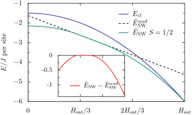
Figure 4: (Color online) The blue curve (triangles) is the classical energy and the green curve (circles) is the new energy curve constructed by extrapolating linearly the energy of the different structures. (Inset) Energy measured with respect to the energy of the uud state.

In this construction the resulting energy curve $\tilde{E}(H)$ is strictly linear in the vicinity of $H_{\textrm{sat}}/3$. This behavior corresponds to the plateau stabilization (see Fig. 4). The plateau width obtained in this approach is reported as a function of $1/S$ in figure 5. The same plot also presents the plateau width estimates of Ref. [Chubukov and Golosov, 1991] as well as the critical fields obtained numerically by cutting the magnetization curve at the value $1/3$. In all cases the agreement with Chubukov and Golosov’s prediction is excellent for large $S$.

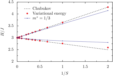
Figure 5: (Color online) Plot the $1/3$ magnetization plateau width as a function of $1/S$ estimated by different approaches. Critical fields determined by: the condition $m=1/3$ (blue curve) and from the variational energy construction $\tilde{E}(H)$ (red points). The plot also presents the extension of the lowest-order Chubukov and Golosov predictionChubukov and Golosov (1991) to all $S$ (dashed lines).

One should note that given the non trivial field dependence of the magnetization curve corrected to first order in $1/S$, solving for $H$ the equation $m(H)=1/3$ yields solutions whose expression as a series in $1/S$ includes powers of $1/S$ greater than one. This explains the discrepancy between the critical field prediction of this approach and that of Chubukov for large values of $1/S$ [see Fig. 5]. Nevertheless, figure 5 is the numerical confirmation that the leading $1/S$ behaviors are the same as predicted analytically.

VI Comparison with experiments

To assess the validity of our magnetization curve construction, we compare it to recent magnetization measurements on different compounds which are the closest known experimental realizations of the Heisenberg model on the triangular lattice. Figure 6 compares the magnetization measurements for the compounds Ba₃CoSb₂O₉, Ba₃NiSb₂O₉ and RbFe(MoO₄)₂ [corresponding to a magnetic moment respectively of $S=1/2$, $S=1$ and $S=5/2$] to our $1/S$ prediction.

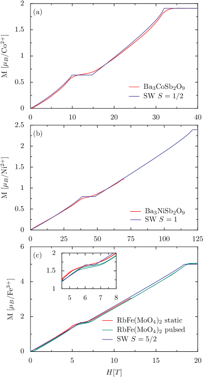
Figure 6: Plot of the magnetization curve measurements for the compounds: Ba₃CoSb₂O₉ ($S=1/2,T=1.3K$, powder sample) Shirata et al. (2012) a), Ba₃NiSb₂O₉ ($S=1/2,T=1.3K$, powder sample) Shirata et al. (2011) b), RbFe(MoO₄)₂ ($S=5/2,T=1.3K$, pulsed field) Smirnov et al. (2007) and RbFe(MoO₄)₂ ($S=5/2,T=1.55K$, static field) Svistov et al. (2003) c) and of the $1/S$ prediction at different values of $S$.

In spite of its simplicity, our theoretical prediction for the magnetization curve which consists in cutting the $1/S$ magnetization at the value $m=1/3$ yields results in good agreement with the experimental data both for the plateau width and position as well as for the magnetization curve away from the plateau. We stress however that our approach mainly provides an understanding of the plateau stabilization in the semiclassical approach. Recent numerical studies for spin-1/2 Yamamoto et al. (2014, 2015); *Sellmann15 done in the context of the magnetization process of Ba₃CoSb₂O₉, including an XXZ anisotropy, are clearly more quantitative. For large spins however, our semiclassical approach is expected to be accurate.

In that respect, we note that, in spite of the larger value of the magnetic moment, the agreement of our prediction with the measurements for $S=5/2$ compound [Fig. 6 c)] is not as good as for the other compounds. We note however some discrepancies between the pulsed and static filed measurements in RbFe(MoO₄)₂. Furthermore, for this compound, the saturation field is much smaller than that of the other systems. So, measured in units of the coupling constant, the effective temperature is much larger, and temperature effects cannot be neglected. The general trend that the plateau is a much smaller anomaly for larger spin is nevertheless supported by the experimental data.

VII Conclusion

In conclusion, we have shown that a semiclassical calculation of the magnetization curve of the Heisenberg model on the triangular lattice which includes the plateau at $1/3$ and which is correct to order $1/S$ can be simply obtained in two steps: i) calculate the magnetization as minus the derivative of the harmonic energy with respect to the field; ii) cut this curve by a horizontal line at $1/3$. The justification of cutting this curve at $1/3$ relies in an essential way on the presence of a kink in the semiclassical energy for the field at which the uud state is stabilized. Thus, this simple method can be generalized to other models, step ii) being replaced by a cut around each point where the semiclassical energy has a kink, with the corresponding magnetization.

Of course, this simple approach does not give access to all details of the magnetization curve. In particular, it leads to cusps with finite slopes at the plateau boundaries, whereas general arguments suggest that the transition into the plateau state should either be of the first order accompanied by a magnetization jump, or continuous and display a logarithmic singularity with an infinite slope since belonging to the same universality class of the transition into the saturated phaseTakano et al. (2011); Zhitomirsky and Nikuni (1998); Gluzman (1993); Fisher and Hohenberg (1988). To access these details requires to go beyond the linear order in the spin wave expansion.

However, as demonstrated by the comparison with experimental data, the present theory is quite accurate even for S=1/2, and it would presumably take experiments at very low temperature in highly isotropic systems to actually observe significant deviations from the present theory, provided of course the system does not realize nonclassical ground states on the way to polarization. Considering the difficulty in pushing spin-wave theory beyond linear order, it is our hope that the present approach, which only relies on the elementary linear spin-wave theory, will be useful to both experimentalists and theorists in the investigation of the magnetization process of frustrated quantum magnets.

Appendix A Spin wave theory

This section presents the explicit expression of some results of the linear spin wave approximation for a generic 3-sublattice coplanar state, as well as some aspects of the calculation to higher order referred to in the text.

A.1 Linear spin wave approximation and $1/S$ magnetization

The block structure of the harmonic fluctuation matrix, $M_{\bf k}$, entering Eq. (6) is detailed below

$$M_{\bf k}=\left(\begin{array}[]{cc}\bar{\bar{A}}_{\bf k}&\bar{\bar{B}}_{\bf k}\\ \bar{\bar{B}}_{\bf k}&\bar{\bar{A}}_{\bf k}\end{array}\right)$$ (19)

with

$$\bar{\bar{A}}_{\bf k}=\left(\begin{array}[]{ccc}A&\gamma_{\bf k}^{\star}D&\gamma_{\bf k}H\\ \gamma_{\bf k}D&B&\gamma_{\bf k}^{\star}F\\ \gamma_{\bf k}^{\star}H&\gamma_{\bf k}F&C\\ \end{array}\right)\quad\textrm{ and }\quad\bar{\bar{B}}_{\bf k}=\left(\begin{array}[]{ccc}0&\gamma_{\bf k}^{\star}E&\gamma_{\bf k}I\\ \gamma_{\bf k}E&0&\gamma_{\bf k}^{\star}G\\ \gamma_{\bf k}^{\star}I&\gamma_{\bf k}G&0\end{array}\right).$$ (20)

The coefficients entering Eq. (20) are:

$$\begin{array}[]{l}A=\left[-3J(\cos{\theta_{1,2}}+\cos{\theta_{1,3}})+H\cos\theta_{1}\right],\\[5.69054pt] B=\left[-3J(\cos{\theta_{1,2}}+\cos{\theta_{2,3}})+H\cos\theta_{2}\right],\\[5.69054pt] C=\left[-3J(\cos{\theta_{1,3}}+\cos{\theta_{2,3}})+H\cos\theta_{3}\right],\\[5.69054pt] D=J(\cos{\theta_{1,2}}+1)/2,\quad E=J(\cos{\theta_{1,2}}-1)/2,\\[5.69054pt] F=J(\cos{\theta_{2,3}}+1)/2,\quad G=J(\cos{\theta_{2,3}}-1)/2,\\[5.69054pt] H=J(\cos{\theta_{1,3}}+1)/2,\quad I=J(\cos{\theta_{1,3}}-1)/2.\end{array}$$ (21)

where $\theta_{i,j}=\theta_{i}-\theta_{j}$ is the difference between the spin orientations on sublattices $i$ and $j$ (see Fig. 1). The geometrical coefficient $\gamma_{\bf k}$ is given by

$$\gamma_{\bf k}=\left(e^{i{\bf k}{\bf a}}+e^{-i{\bf k}{\bf b}}+e^{i{\bf k}(-\bf{a}+{\bf b})}\right),\\$$ (22)

for the triangular lattice basis vectors ${\bf a}$ and ${\bf b}$ defined in Fig. 1a). The additional term $\Delta_{\bf k}$ in Eq. (6) is equal to the trace of $\bar{\bar{A}}_{\bf k}$, $\Delta_{\bf k}=\textrm{Tr}[\bar{\bar{A}}_{\bf k}]$.

The Bogolyubov transformation which diagonalizes (6) consists of a $6\times 6$ momentum dependent matrix, $T_{\bf k}$, with block structure

$$T_{\bf k}=\left(\begin{array}[]{cc}U_{\bf k}&V_{\bf k}\\ V_{\bf k}&U_{\bf k}\end{array}\right)\,.$$ (23)

For any value of momenta, $T_{\bf k}$ simultaneously fulfills the conditions that: i) $T^{\dagger}_{\bf k}M_{\bf k}T_{\bf k}$ is diagonal with doubly degenerate, real positive eigenvalues $\omega_{{\bf k},n}$

$$\begin{array}[]{c}T^{\dagger}_{\bf k}M_{\bf k}T_{\bf k}=\Omega_{\bf k}\,,\\[8.53581pt] \Omega_{\bf k}=\left(\begin{array}[]{cc}\omega_{\bf k}&0\\ 0&\omega_{\bf k}\end{array}\right)\,\textrm{ with }\,\omega_{\bf k}=\left(\begin{array}[]{ccc}\omega_{{\bf k},1}&0&0\\ 0&\omega_{{\bf k},2}&0\\ 0&0&\omega_{{\bf k},3}\end{array}\right)\,,\end{array}$$ (24)

and ii) that

$$YT_{\bf k}YT_{\bf k}^{\dagger}=\mathbb{I}\,,\textrm{ with }Y=\left(\begin{array}[]{cc}\mathbb{I}&0\\ 0&-\mathbb{I}\end{array}\right)\,.$$ (25)

In terms of the blocks $U_{\bf k}$ and $V_{\bf k}$, this amounts to meeting the two following requirements

$$\begin{array}[]{ll}U_{\bf k}U_{\bf k}^{\dagger}-V_{\bf k}V_{\bf k}^{\dagger}=\mathbb{I}\,,\\[5.69054pt] U_{\bf k}V_{\bf k}^{\dagger}-V_{\bf k}U_{\bf k}^{\dagger}=0\,.\end{array}$$ (26)

This condition (26) ensures that the Bogolyubov quasiparticles, which are linear combinations of the bosonic fields $a_{{\bf k},n}$ and $a_{{\bf k},n}^{\dagger}$, also obey bosonic statistics.

The zero point energy per site can be expressed in terms of $T_{\bf k}$ as

$$\delta E=\frac{1}{2SN}\sum_{\bf k}{\frac{1}{2}\textrm{Tr}\left[T^{\dagger}_{\bf k}M_{\bf k}T_{\bf k}\right]-\textrm{Tr}\left[\bar{\bar{A}}_{\bf k}\right]}\,.$$ (27)

According to Eq. (8), the $1/S$ correction to the magnetization, $\delta m$, is equal to minus the derivative of (27) with respect to the magnetic field $H$. Given that $\textrm{Tr}[\bar{\bar{A}}_{\bf k}]=9J$ for both the Y and V states one obtains

$$\delta m=-\frac{1}{2SN}\sum_{\bf k}{\frac{1}{2}\textrm{Tr}\left[T^{\dagger}_{\bf k}\frac{\partial M_{\bf k}}{\partial H}T_{\bf k}+\frac{\partial T^{\dagger}_{\bf k}}{\partial H}M_{\bf k}T_{\bf k}+T^{\dagger}_{\bf k}M_{\bf k}\frac{\partial T_{\bf k}}{\partial H}\right]}\,.$$ (28)

Using Eq. (24), the cyclic property of the trace, and the normalization condition (26) one can show that the last two terms in (28) vanish

$$\begin{array}[]{c}\displaystyle\textrm{Tr}\left[\frac{\partial T^{\dagger}_{\bf k}}{\partial H}M_{\bf k}T_{\bf k}+T^{\dagger}_{\bf k}M_{\bf k}\frac{\partial T_{\bf k}}{\partial H}\right]\\[8.53581pt] =\displaystyle\textrm{Tr}\left[\Omega_{\bf k}\left(\frac{\partial T^{\dagger}_{\bf k}}{\partial H}YT_{\bf k}Y+YT^{\dagger}_{\bf k}Y\frac{\partial T_{\bf k}}{\partial H}\right)\right]\\[8.53581pt] =\displaystyle\textrm{Tr}\left[\Omega_{\bf k}\frac{\partial}{\partial H}\left(\begin{array}[]{cc}U_{\bf k}U_{\bf k}^{\dagger}-V_{\bf k}V_{\bf k}^{\dagger}&U_{\bf k}V_{\bf k}^{\dagger}-V_{\bf k}U_{\bf k}^{\dagger}\\ U_{\bf k}V_{\bf k}^{\dagger}-V_{\bf k}U_{\bf k}^{\dagger}&U_{\bf k}U_{\bf k}^{\dagger}-V_{\bf k}V_{\bf k}^{\dagger}\\ \end{array}\right)\right]=0\,.\end{array}$$ (29)

The cancellation of the terms above, which is due to the normalization conditions of the eigenvectors of $M_{\bf k}$, is analogous to that occurring in the Hellmann-Feynman theorem. Hence, the $1/S$ expression for the magnetization is given by

$$\delta m=-\frac{1}{2SN}\sum_{\bf k}{\frac{1}{2}\textrm{Tr}\left[T^{\dagger}_{\bf k}\frac{\partial M_{\bf k}}{\partial H}T_{\bf k}\right]}\,,$$ (30)

which, given the block structure of $T_{\bf k}$, can be conveniently rewritten as

$$\delta m=-\frac{1}{SN}\sum_{\bf k}\textrm{Tr}\left[\frac{\partial\bar{\bar{A}}_{\bf k}}{\partial H}V_{\bf k}V^{\dagger}_{\bf k}+\frac{\partial\bar{\bar{B}}_{\bf k}}{\partial H}U_{\bf k}V^{\dagger}_{\bf k}\right]\,.$$ (31)

The derivative with respect to the field of the coefficients of $\bar{\bar{A}}_{\bf k}$ and $\bar{\bar{B}}_{\bf k}$ yields

$$\frac{\partial\bar{\bar{A}}_{\bf k}^{Y}}{\partial H}=\frac{\partial\bar{\bar{B}}_{\bf k}^{Y}}{\partial H}=\left(\begin{array}[]{ccc}0&-\gamma_{\bf k}^{\star}/12&-\gamma_{\bf k}/12\\ -\gamma_{\bf k}/12&0&\gamma_{\bf k}^{\star}\cos\theta_{2}^{Y}/3\\ -\gamma_{\bf k}^{\star}/12&\gamma_{\bf k}\cos\theta_{2}^{Y}/3&0\\ \end{array}\right)\,,$$ (32)

for the Y state, and

$$\frac{\partial\bar{\bar{A}}_{\bf k}^{V}}{\partial H}=\frac{\partial\bar{\bar{B}}_{\bf k}^{V}}{\partial H}=\frac{H}{36J}\left(\begin{array}[]{ccc}0&-\gamma_{\bf k}^{\star}&-\gamma_{\bf k}\\ -\gamma_{\bf k}&0&0\\ -\gamma_{\bf k}^{\star}&0&0\\ \end{array}\right)\,,$$ (33)

for the V state. To make contact with the alternative method to compute the $1/S$ magnetization presented in the main text, we note that the two body averages introduced in Eq. (11) are given by the following Brillouin zone integrals

$$\begin{array}[]{l}\displaystyle n_{i}=\langle a_{{\bf R},i}^{\dagger}a_{{\bf R},i}^{\phantom{\dagger}}\rangle=\frac{3}{N}\sum_{\bf k}\left(V_{\bf k}^{\phantom{\dagger}}V^{\dagger}_{\bf k}\right)_{i,i}\,\,,\\ \displaystyle m_{ij}=\langle a_{{\bf R},i}^{\dagger}a_{{\bf R^{\prime}},j}^{\phantom{\dagger}}\rangle=\frac{1}{N}\sum_{\bf k}\gamma_{\bf k}\left(V_{\bf k}^{\phantom{\dagger}}V^{\dagger}_{\bf k}\right)_{i,j}\,,\\ \displaystyle\Delta_{ij}=\langle a_{{\bf R},i}^{\phantom{\dagger}}a_{{\bf R^{\prime}},j}^{\phantom{\dagger}}\rangle=\frac{1}{N}\sum_{\bf k}\gamma_{\bf k}\left(U_{\bf k}^{\phantom{\dagger}}V^{\dagger}_{\bf k}\right)_{i,j}\,,\\ \end{array}$$ (34)

with the sites $({\bf R},i)$ and $({\bf R^{\prime}},j)$ being nearest neighbors. The field dependence of the averages $n_{i},m_{ij}$ and $\Delta_{ij}$ is reported in Fig. 7. The symmetries of the Y and V structures yield $n_{2}=n_{3}$, $m_{12}=m_{13}$ , and $\Delta_{12}=\Delta_{13}$.

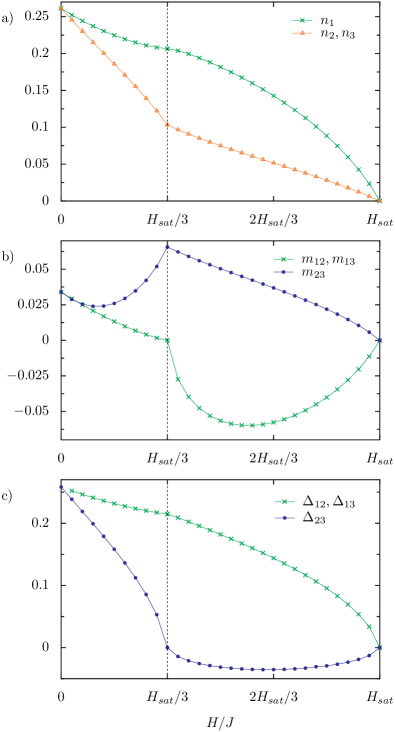
Figure 7: (Color online) Plot, as a function of the magnetic field, of the average quantities $n_{i}=\langle a_{{\bf R},i}^{\dagger}a_{{\bf R},i}\rangle$ panel a), $m_{ij}=\langle a_{{\bf R},i}^{\dagger}a_{{\bf R^{\prime}},j}\rangle$ panel b), $\Delta_{ij}=\langle a_{{\bf R},i}a_{{\bf R^{\prime}},j}\rangle$ panel c). We note that at $H=H_{\rm sat}/3$, i.e. for the uud state, the quantum corrections to the magnetization exactly compensate, that is $n_{1}-2n_{2}=0$.

Injecting Eqs. (32), (33), and (34) into Eq. (31) one recovers the $1/S$ contribution to the magnetization presented in Eq. (13), which is reminded below

$$\begin{array}[]{l}\displaystyle\delta m^{Y}=\frac{1}{3S}\left(-2\cos\theta_{2}^{Y}(m_{23}+\Delta_{23})+m_{21}+\Delta_{21}\right)\,,\\[8.53581pt] \displaystyle\delta m^{V}=-\frac{1}{S}\frac{H}{9J}\left(\Delta_{21}+m_{21}\right)\,.\end{array}$$ (35)

A.2 Spectrum renormalization of the uud state

The 3-sublattice uud structure turns out to be classically stable at $H=H_{\textrm{sat}}/3$. Since, according to order by disorder, collinear configurations tend to have a softer spectrum, hence a smaller zero-point energy Shender (1982a); *Shender2; Henley (1989), quantum fluctuations stabilize this uud state over a finite field range around $H_{\textrm{sat}}/3$ leading to the $1/3$ magnetization plateau Chubukov and Golosov (1991). For the specific field value $H_{\textrm{sat}}/3$, the harmonic spectrum of the $1/S$ expansion turns out to have two gapless low energy modes and a higher energy gapped mode. If the uud state is to be stabilized over a given field range, it should be gapped to spin excitations. Chubukov and GolosovChubukov and Golosov (1991) showed that treating self consistently the higher order terms in the spin wave expansion yields an excitation spectrum in which the two lowest bands are gapped. For completeness we reproduce the main steps which lead Chubukov and Golosov to this conclusion.

Because of collinearity, the next non vanishing term in the $1/S$ expansion around the uud state is quartic in boson operators. Decoupling the quartic terms [of order $\mathcal{O}(1/S^{2})$] yields an effective harmonic Hamiltonian which, up to a constant, is given by

$$\mathcal{H}^{\textrm{eff}}=NE_{\textrm{cl}}^{\textrm{uud}}+\frac{1}{2S}\sum_{\bf k}{\bf a}_{\bf k}^{\dagger}\left[M_{\bf k}^{\textrm{uud}}(H)+\frac{1}{S}M_{\bf k}^{\textrm{eff}}\right]{\bf a}_{\bf k}^{\phantom{\dagger}}\ ,$$ (36)

where $M_{\bf k}^{\textrm{eff}}$ has the same block structure as $M_{\bf k}$ (19). The sub-blocks of $M_{\bf k}^{\textrm{eff}}$ are denoted by $\bar{\bar{A}}_{\bf k}^{\textrm{eff}}$ and $\bar{\bar{B}}_{\bf k}^{\textrm{eff}}$. Their expression can be obtained by replacing into Eq. (20) the following coefficients

$$\begin{array}[]{l}A^{\textrm{eff}}=6J(-\bar{n}_{2}+\bar{\Delta}_{21})\,,\\[5.69054pt] B^{\textrm{eff}}=C^{\textrm{eff}}=3J(-\bar{n}_{1}+\bar{n}_{2}+\bar{\Delta}_{21}-\bar{m}_{23})\,,\\[5.69054pt] F^{\textrm{eff}}=J(\bar{m}_{23}-\bar{n}_{2})\,,\quad D^{\textrm{eff}}=G^{\textrm{eff}}=H^{\textrm{eff}}=0\,,\\[5.69054pt] E^{\textrm{eff}}=I^{\textrm{eff}}=J(-\bar{\Delta}_{21}+(\bar{n}_{1}+\bar{n}_{2})/2)\,,\end{array}$$ (37)

where the averages $n_{i},m_{ij}$ and $\Delta_{ij}$ have been defined in Eq. (11) [see Fig. 7]. The bar superscript specifies that the average quantities are computed for the field $H=H_{\textrm{sat}}/3$.

The contribution of the quartic terms renormalizes the harmonic spectrum opening two gaps at ${\bf k}=0$

$$\begin{array}[]{l}\displaystyle\omega_{\bf 0}^{(1)}\approx\frac{1}{S}\left[H-3J\left(1+\frac{2\bar{m}_{23}-\bar{\Delta}_{21}}{S}\right)\right]+\mathcal{O}(S^{-3})\,,\\[8.53581pt] \displaystyle\omega_{\bf 0}^{(2)}\approx\frac{1}{S}\left[-H+3J\left(1+\frac{\bar{\Delta}_{21}}{S}\right)\right]+\mathcal{O}(S^{-3})\,.\end{array}$$ (38)

The instability of the uud structure is resolved by determining the fields at which the gaps to the first excited states close. To first order in $1/S$, the expression of the field values at which this takes place coincides with that given in Eq. (15). Ref. [Takano et al., 2011] provides a refinement of this approach which consists of a self consistent treatment of the decoupling of quartic terms.

Appendix B Variational energy envelope

In this Appendix we briefly mention some details of the calculation leading to the construction of a new energy curve which supports the $1/3$ magnetization plateau in the triangular lattice Heisenberg antiferromagnet. Let us first introduce the following notations to specify the different terms entering Eq. (17)

$$\langle\phi_{0}|\mathcal{H}(H_{0})|\phi_{0}\rangle=E_{cl}(H_{0})+\frac{1}{S}\delta E(H_{0})\,,$$ (39)

where $E_{cl}(H_{0})$ is the classical energy at $H=H_{0}$ and $\delta E(H_{0})/S$ the $1/S$ corrections to it. For states different from the uud structure, the magnetization, correct to order $1/S$, is obtained by deriving (39) with respect to the field $H_{0}$

$$\begin{array}[]{lll}m(H_{0})&=&\displaystyle-\frac{\partial}{\partial H_{0}}\left(E_{cl}(H_{0})+\frac{1}{S}\delta E(H_{0})\right)\\[8.53581pt] &=&\displaystyle m_{cl}(H_{0})+\frac{1}{S}\delta m(H_{0})\,,\end{array}$$ (40)

where $m_{cl}(H_{0})$ is the classical magnetization and $\delta m(H_{0})/S$ the $1/S$ corrections to it. Note that Eq. (40) is meaningless at $H_{\textrm{sat}}/3$. In fact, for this value of the field the harmonic energy presents a cusp and its derivative is not well defined.

The new energy curve which is proposed Eq. (18) consists of the lower envelope of all the energies defined in Eq. (17). As mentioned in the main text, to compare the energies of states to order $1/S$ only the classical contribution to $\langle\phi_{0}|\sum_{i}S_{i}^{z}/S|\phi_{0}\rangle$ should be retained. Thus, the minimization of (18) with respect to $H_{0}$ (again for $H_{0}\neq H_{\textrm{sat}}/3$) gives

$$\begin{array}[]{l}\displaystyle\frac{\partial}{\partial H_{0}}\left(E_{cl}(H_{0})+\frac{1}{S}\delta E(H_{0})\right)+\left(1-(H-H_{0})\frac{\partial}{\partial H_{0}}\right)m_{cl}(H_{0})=0\\ \displaystyle\Rightarrow(H-H_{0})=-\frac{1}{S}\delta m(H_{0})\left(\frac{\partial m_{cl}(H_{0})}{\partial H_{0}}\right)^{-1}\\ \displaystyle\Rightarrow(H-H_{0})=-\frac{1}{S}\frac{\delta m(H_{0})}{\chi_{cl}}\,,\end{array}$$ (41)

where we have introduced the classical susceptibility $\chi_{cl}=\partial m(H)_{cl}/\partial H$ (note that $\chi_{cl}$ is a constant since the classical magnetization depends linearly with the magnetic field). Equation (41) establishes that the difference $H-H_{0}$ which minimizes (18) behaves as $1/S$. Retaining the $1/S$ corrections of $\langle\phi_{0}|\sum_{i}S_{i}^{z}/S|\phi_{0}\rangle$ in the calculation would have produced a $1/S^{2}$ correction to (41).

Next we will show that, away from the plateau, the magnetization defined as the derivative with respect to the field of the new energy envelope $\tilde{E}(H)$ differs from the $1/S$ magnetization (13) only by terms of order $\mathcal{O}(1/S^{2})$. For this purpose, let us compute

$$\tilde{m}(H)=-\frac{\partial\tilde{E}(H_{0}(H))}{\partial H}\,,$$ (42)

where $\tilde{E}(H_{0}(H))$ is the new energy curve with $H_{0}(H)$ denoting the value of $H_{0}$ fulfilling (18) at a given field $H$. After derivation one obtains

$$\begin{array}[]{lll}\tilde{m}(H)&=&\displaystyle-\left[\frac{\partial}{\partial H_{0}}\left(E_{cl}(H_{0}(H))+\frac{1}{S}\delta E(H_{0}(H))\right)\frac{\partial H_{0}}{\partial H}\right.\\[8.53581pt] &&\displaystyle\quad\left.-\left(1-\frac{\partial H_{0}}{\partial H}\right)m_{cl}(H_{0}(H))\right.\\ &&\displaystyle\quad\left.-(H-H_{0})\frac{\partial m_{cl}(H_{0}(H))}{\partial H_{0}}\frac{\partial H_{0}}{\partial H}\right]\\[8.53581pt] &=&m_{cl}(H_{0}(H))\,,\end{array}$$ (43)

where we have used the first line of Eq. (41) to simplify the expression. Thus, in this construction, we are left with a new magnetization curve

$$\tilde{m}(H)=\chi_{cl}H_{0}(H)\,.$$ (44)

The minimization of (18) does not yield a closed form $H_{0}(H)$, however, starting from (41) it is straightforward to see that in the large $S$ limit we have

$$H_{0}=H+\frac{1}{S}\frac{\delta m(H)}{\chi_{cl}}+\mathcal{O}(1/S^{2})\,.$$ (45)

Substituting (45) into (44) produces the result announced earlier

$$\begin{array}[]{lll}\displaystyle\tilde{m}(H)&=&\displaystyle m_{cl}(H)+\frac{1}{S}\delta m(H)+\mathcal{O}(1/S^{2})\\[8.53581pt] &=&\displaystyle m(H)+\mathcal{O}(1/S^{2})\,.\end{array}$$ (46)

So we conclude that away from the plateau, the magnetization associated with the energy curve $\tilde{E}(H)$ differs from the $1/S$ magnetization (13) only by terms of order $\mathcal{O}(1/S^{2})$.

References

- Lacroix et al. (2011) C. Lacroix, P. Mendels, and F. Mila, eds., Introduction to Frustrated Magnetism (Springer, Berlin, 2011).
- Totsuka (1998) K. Totsuka, Phys. Rev. B 57, 3454 (1998).
- Mila (1998) F. Mila, Eur. Phys. J. B 6, 201 (1998).
- Corboz and Mila (2014) P. Corboz and F. Mila, Phys. Rev. Lett. 112, 147203 (2014).
- Cabra et al. (2005) D. C. Cabra, M. D. Grynberg, P. C. W. Holdsworth, A. Honecker, P. Pujol, J. Richter, D. Schmalfuß, and J. Schulenburg, Phys. Rev. B 71, 144420 (2005).
- Capponi et al. (2013) S. Capponi, O. Derzhko, A. Honecker, A. M. Läuchli, and J. Richter, Phys. Rev. B 88, 144416 (2013).
- Nishimoto et al. (2013) S. Nishimoto, N. Shibata, and C. Hotta, Nat. Commun. 4:2287 (2013), http://dx.doi.org/10.1038/ncomms3287.
- Kawamura (1984) H. Kawamura, Journal of the Physical Society of Japan 53, 2452 (1984).
- Chubukov and Golosov (1991) A. V. Chubukov and D. A. Golosov, J. Phys. Condens. Matter 3, 69 (1991).
- Zhitomirsky et al. (2000) M. E. Zhitomirsky, A. Honecker, and O. A. Petrenko, Phys. Rev. Lett. 85, 3269 (2000).
- Penc et al. (2004) K. Penc, N. Shannon, and H. Shiba, Phys. Rev. Lett. 93, 197203 (2004).
- Coletta et al. (2013) T. Coletta, M. E. Zhitomirsky, and F. Mila, Phys. Rev. B 87, 060407 (2013).
- Honecker et al. (2004) A. Honecker, J. Schulenburg, and J. Richter, J. Phys. Condens. Matter 16, S749 (2004).
- Shirata et al. (2011) Y. Shirata, H. Tanaka, T. Ono, A. Matsuo, K. Kindo, and H. Nakano, Journal of the Physical Society of Japan 80, 093702 (2011).
- Richter et al. (2013) J. Richter, O. Götze, R. Zinke, D. J. J. Farnell, and H. Tanaka, Journal of the Physical Society of Japan 82, 015002 (2013).
- Farnell et al. (2009) D. J. J. Farnell, R. Zinke, J. Schulenburg, and J. Richter, J. Phys. Condens. Matter 21, 406002 (2009).
- Ono et al. (2003) T. Ono, H. Tanaka, H. Aruga Katori, F. Ishikawa, H. Mitamura, and T. Goto, Phys. Rev. B 67, 104431 (2003).
- Ono et al. (2004) T. Ono, H. Tanaka, O. Kolomiyets, H. Mitamura, T. Goto, K. Nakajima, A. Oosawa, Y. Koike, K. Kakurai, J. Klenke, P. Smeibidle, and Meißner, J. Phys. Condens. Matter 16, S773 (2004).
- Tsujii et al. (2007) H. Tsujii, C. R. Rotundu, T. Ono, H. Tanaka, B. Andraka, K. Ingersent, and Y. Takano, Phys. Rev. B 76, 060406 (2007).
- Fortune et al. (2009) N. A. Fortune, S. T. Hannahs, Y. Yoshida, T. E. Sherline, T. Ono, H. Tanaka, and Y. Takano, Phys. Rev. Lett. 102, 257201 (2009).
- Shirata et al. (2012) Y. Shirata, H. Tanaka, A. Matsuo, and K. Kindo, Phys. Rev. Lett. 108, 057205 (2012).
- Susuki et al. (2013) T. Susuki, N. Kurita, T. Tanaka, H. Nojiri, A. Matsuo, K. Kindo, and H. Tanaka, Phys. Rev. Lett. 110, 267201 (2013).
- Svistov et al. (2003) L. E. Svistov, A. I. Smirnov, L. A. Prozorova, O. A. Petrenko, L. N. Demianets, and A. Y. Shapiro, Phys. Rev. B 67, 094434 (2003).
- Svistov et al. (2006) L. E. Svistov, A. I. Smirnov, L. A. Prozorova, O. A. Petrenko, A. Micheler, N. Büttgen, A. Y. Shapiro, and L. N. Demianets, Phys. Rev. B 74, 024412 (2006).
- Smirnov et al. (2007) A. I. Smirnov, H. Yashiro, S. Kimura, M. Hagiwara, Y. Narumi, K. Kindo, A. Kikkawa, K. Katsumata, A. Y. Shapiro, and L. N. Demianets, Phys. Rev. B 75, 134412 (2007).
- Kenzelmann et al. (2007) M. Kenzelmann, G. Lawes, A. B. Harris, G. Gasparovic, C. Broholm, A. P. Ramirez, G. A. Jorge, M. Jaime, S. Park, Q. Huang, A. Y. Shapiro, and L. A. Demianets, Phys. Rev. Lett. 98, 267205 (2007).
- White et al. (2013) J. S. White, C. Niedermayer, G. Gasparovic, C. Broholm, J. M. S. Park, A. Y. Shapiro, L. A. Demianets, and M. Kenzelmann, Phys. Rev. B 88, 060409 (2013).
- Zhitomirsky and Nikuni (1998) M. E. Zhitomirsky and T. Nikuni, Phys. Rev. B 57, 5013 (1998).
- Note (1) The choice of renormalizing the bilinear spin coupling by and the magnetic field by formally allows to replace the quantum spin operators by three dimensional classical vectors of norm in the limit. Furthermore, this choice leads to a simple and transparent dependence in of the different terms of the spin wave expansion.
- Holstein and Primakoff (1940) T. Holstein and H. Primakoff, Phys. Rev. 58, 1098 (1940).
- Nikuni and Shiba (1993) T. Nikuni and H. Shiba, Journal of the Physical Society of Japan 62, 3268 (1993).
- Hellmann (1937) H. Hellmann, Einfüührung in die Quantenchemie (Franz Deuticke, Leipzig, 1937).
- Feynman (1939) R. P. Feynman, Phys. Rev. 56, 340 (1939).
- Jacobs et al. (1993) A. Jacobs, T. Nikuni, and H. Shiba, Journal of the Physical Society of Japan 62, 4066 (1993).
- Note (2) The superscript bar is used to emphasize that the averages , and are computed at . The bar is omitted when averages are computed at different fields.
- Yamamoto et al. (2014) D. Yamamoto, G. Marmorini, and I. Danshita, Phys. Rev. Lett. 112, 127203 (2014).
- Yamamoto et al. (2015) D. Yamamoto, G. Marmorini, and I. Danshita, Phys. Rev. Lett. 114, 027201 (2015).
- Sellmann et al. (2015) D. Sellmann, X.-F. Zhang, and S. Eggert, Phys. Rev. B 91, 081104 (2015).
- Takano et al. (2011) J. Takano, H. Tsunetsugu, and M. E. Zhitomirsky, J. Phys. Conf. Ser. 320, 012011 (2011).
- Gluzman (1993) S. Gluzman, Zeitschrift für Physik B Condensed Matter 90, 313 (1993).
- Fisher and Hohenberg (1988) D. S. Fisher and P. C. Hohenberg, Phys. Rev. B 37, 4936 (1988).
- Shender (1982a) E. F. Shender, ZhETF 83, 326 (1982a).
- Shender (1982b) E. F. Shender, Sov. Phys. JETP 56, 178 (1982b).
- Henley (1989) C. L. Henley, Phys. Rev. Lett. 62, 2056 (1989).