A new approach of the Chebyshev wavelets for the variable-order time fractional mobile-immobile advection-dispersion model

Abstract

This paper proposes a new numerical method based on the Chebyshev wavelets (CWs) to solve the variable-order time fractional mobile-immobile advection-dispersion equation. To do this, a new operational matrix of variable-order fractional derivative in the Caputo sense for the CWs is derived and is used to obtain an approximate solution for the problem under study. Along the way a new family of piecewise functions is introduced and employed to derive a general method to compute this matrix. The main advantage behind the proposed approach is that the problem under consideration is transformed into a linear system of algebraic equations. So, it can be solved simply to obtain an approximate solution. The efficiency and accuracy of the proposed method are shown for some concrete examples. These results show that the proposed method is very efficient and accurate.

Keywords: Chebyshev wavelets (CWs); Operational matrix of variable-order fractional derivative; Variable-order time fractional mobile-immobile advection-dispersion equation; Caputo’s variable-order fractional derivative.

Mathematics Subject Classification 2010: 35R11.

1 Introduction

Variable-order fractional derivatives, which are an extension of constant-order fractional ones have been introduced in several physical applications [1, 2, 3]. Recently, some researchers [4, 5, 6, 7, 8, 9, 10, 11] have shown that many complex physical models can be described via variable-order derivatives with a great success. It is worth noting that analytically handling equations described by the variable-order fractional derivatives is difficult due to their highly complex, so proposing efficient methods to find their numerical solutions is of great importance in practical. So, recently several methods have been proposed to solve variable-order fractional differential equations numerically such as [12, 13, 14, 15, 16, 17, 18, 19, 20, 21, 22, 23, 24, 25, 26, 27].
Wavelets theory which is a relatively new area in mathematical research has been applied in a wide range of engineering disciplines [28]. In recent years, wavelets have been applied for solving different types of partial differential equations e.g. [28, 29, 30, 31].
The aim of this paper is to propose a new numerical method based on the CWs to solve the following variable-order time fractional mobile-immobile advection-dispersion model [32]:

$$\alpha_{1}\frac{\partial u(x,t)}{\partial t}+\alpha_{2}\,\prescript{c}{0}{D_{t}^{\gamma(x,t)}}u(x,t)=-\mu_{1}\frac{\partial u(x,t)}{\partial x}+\mu_{2}\frac{\partial^{2}u(x,t)}{\partial x^{2}}+f(x,t),\hskip 14.22636pt(x,t)\in\Omega,$$ (1.1)

with $\Omega=[0,1]\times[0,1]$, subject to the following initial-boundary conditions:

$$\begin{array}[]{ll}u(x,0)=g(x),&\\ \vskip 6.0pt plus 2.0pt minus 2.0pt\cr u(0,t)=h_{1}(t),&u(1,t)=h_{2}(t),\end{array}$$ (1.2)

where $\alpha_{1}\geq 0$, $\alpha_{2}\geq 0$, $\mu_{1}>0$, $\mu_{2}>0$, $0<\gamma(x,t)\leq 1$, $f(x,t)$, $g(x)$, $h_{1}(t)$ and $h_{2}(t)$ are given functions, and $\prescript{c}{0}{D_{t}^{\gamma(x,t)}}$ denotes the variable-order fractional derivatives in the Caputo sense of order $0<\gamma(x,t)\leq 1$, as defined by [19, 20]:

$$\prescript{c}{0}{D_{t}^{\gamma(x,t)}}u(x,t)=\frac{1}{\Gamma\left(1-\gamma(x,t)\right)}\int_{0}^{t}\left(t-s\right)^{-\gamma(x,t)}\frac{\partial u(x,s)}{\partial s}ds,\hskip 14.22636ptt>0.$$ (1.3)

It is worth noting that based on the definition of the variable-order fractional derivative in the Caputo sense as [20], we have the following useful property:

$$\prescript{c}{0}{D_{t}^{\vartheta(x,t)}}t^{m}=\displaystyle\left\{\begin{array}[]{cl}\displaystyle\frac{\Gamma(m+1)}{\Gamma(m-\vartheta(x,t)+1)}\,t^{m-\vartheta(x,t)},&q\leq m\in\mathbb{N},\\ \vskip 6.0pt plus 2.0pt minus 2.0pt\cr 0,&o.w,\end{array}\right.$$ (1.4)

where $q-1<\vartheta(x,t)\leq q$.
To solve equation in (1.1), we first derive a new operational matrix of variable-order fractional derivative in the Caputo sense for the CWs and then, employ this matrix to obtain an approximate solution for the problem at hand. Along the way, a new family of piecewise functions is introduced and employed to derive a general procedure for forming this matrix.
In the proposed method, at first the solution of the problem at hand is expanded in terms of the CWs. Then, by computing the operational matrix of variable-order fractional derivative and using some properties of these basis polynomials, we transform its solution to the solution of a linear system of algebraic equations. This greatly simplifies the process of solving the problem as well as help to achieve an approximate solution for the problem.
The remainder of this paper is organized as follows: In section 2, the CWs and their properties are introduced. In section 3, the operational matrix of variable-order fractional derivative for the CWs is derived and in section 4, the proposed method is described for solving the problem under study. Section 5, contains some numerical examples which are solved using the proposed method. Finally, a conclusion is given in section 6.

2 The CWs and their properties

Wavelets constitute a family of functions constructed from dilation and translation of a single function $\psi(t)$ called the mother wavelet. When the dilation parameter $a$ and the translation parameter $b$ vary continuously we have the following family of continuous wavelets as:

$$\psi_{ab}(t)=|a|^{-\frac{1}{2}}\psi\left(\frac{t-b}{a}\right),\hskip 14.22636pta,\,b\in\mathbb{R},\,\,a\neq 0.$$ (2.1)

If we restrict the parameters $a$ and $b$ to discrete values as $a=a_{0}^{-k}$, $b=nb_{0}a_{0}^{-k}$, where $a_{0}>1$, $b_{0}>0$, we have the following family of discrete wavelets

$$\psi_{kn}(t)=|a_{0}|^{\frac{k}{2}}\psi\left(a_{0}^{k}t-nb_{0}\right),\hskip 14.22636ptk,\,n\in\mathbb{Z},$$ (2.2)

where the functions $\psi_{kn}(t)$ form a wavelet basis for $L^{2}(\mathbb{R})$.
In practice, when $a_{0}=2$ and $b_{0}=1$, the functions $\psi_{kn}(t)$ form an orthonormal basis.
The CWs are defined on the interval $[0,1]$ by [33, 34]:

$$\psi_{nm}(t)=\displaystyle\left\{\begin{array}[]{ccl}\displaystyle\beta_{m}2^{\frac{k}{2}}T^{\ast}_{m}\left(2^{k}t-n\right),&&\displaystyle t\in\left[\frac{n}{2^{k}},\frac{n+1}{2^{k}}\right],\\ \vskip 6.0pt plus 2.0pt minus 2.0pt\cr 0,&&o.w,\end{array}\right.$$ (2.3)

for $n=0,1,\ldots,2^{k}-1$, $m=0,1,\ldots,M-1$, $(k,M)\in\mathbb{N}$, where

$$\beta_{m}=\displaystyle\left\{\begin{array}[]{ccc}\displaystyle\sqrt{\frac{2}{\pi}},&&m=0,\\ \vskip 6.0pt plus 2.0pt minus 2.0pt\cr\displaystyle\frac{2}{\sqrt{\pi}},&&m\geq 1,\end{array}\right.$$ (2.4)

and $T^{\ast}_{m}(t)$ denotes the shifted Chebyshev polynomials, which are defined on the interval $[0,1]$ as:

$$\begin{array}[]{l}\displaystyle T^{\ast}_{0}(t)=1,\\ \vskip 6.0pt plus 2.0pt minus 2.0pt\cr\displaystyle T^{\ast}_{m}(t)=m\sum_{i=0}^{m}(-1)^{m-i}\frac{2^{2i}(m+i-1)!}{(m-i)!(2i)!}\,t^{i},\hskip 14.22636ptm=1,2,\ldots.\end{array}$$ (2.5)

The set of the CWs is an orthogonal set with respect to the weight function $w_{n}(t)$ where

$$w_{n}(t)=\left\{\begin{array}[]{ccl}\displaystyle\frac{1}{\sqrt{1-\left(2^{k+1}t-2n-1\right)^{2}}},&&\displaystyle t\in\left[\frac{n}{2^{k}},\frac{n+1}{2^{k}}\right],\\ \vskip 6.0pt plus 2.0pt minus 2.0pt\cr 0,&&o.w.\end{array}\right.$$ (2.6)

The CWs can be used to expand any function $u(t)$ which is defined over $[0,1]$ as:

$$u(t)=\sum_{n=0}^{\infty}\sum_{m=0}^{\infty}{c_{nm}\psi_{nm}(t)},$$ (2.7)

where $c_{nm}=\left<u(t),\psi_{nm}(t)\right>$ and $\left<.,.\right>$ denotes the inner product in $L_{w_{n}}^{2}[0,1]$.
By truncating the infinite series in equation (2.7), $u(t)$ is approximated as:

$$u(t)\simeq\sum_{n=0}^{2^{k}-1}\sum_{m=0}^{M-1}{c_{nm}\psi_{nm}(t)=C^{T}\Psi(t)},$$ (2.8)

where $C$ and $\Psi(t)$ are column vectors with $\hat{m}=2^{k}M$ elements.
For simplicity, equation (2.8) is written as:

$$u(t)\simeq\sum_{i=1}^{\hat{m}}{c_{i}\psi_{i}(t)=C^{T}\Psi(t)},$$ (2.9)

where $c_{i}=c_{nm}$ and $\psi_{i}(t)=\psi_{nm}(t)$, and the index $i$ is calculated as $i=Mn+m+1$.
Thus, we have:

$$C\triangleq\left[c_{1},c_{2},\ldots,c_{\hat{m}}\right]^{T},$$

$$\Psi(t)\triangleq\left[\psi_{1}(t),\psi_{2}(t),\ldots,\psi_{\hat{m}}(t)\right]^{T}.$$ (2.10)

Similarly, the CWs can be used to expand an arbitrary function of two variables such as $u(x,t)$ which is defined over $[0,1]\times[0,1]$ as:

$$u(x,t)\simeq\sum_{i=1}^{\hat{m}}\sum_{j=1}^{\hat{m}}u_{ij}\psi_{i}(x)\psi_{j}(t)=\Psi^{T}(x)\textbf{U}\Psi(t),$$ (2.11)

where $U=[u_{ij}]$ and $u_{ij}=\left(\psi_{i}(x),\left(u(x,t),\psi_{j}(t)\right)\right)$.
The derivative of the vector $\Psi(t)$ defined in equation (2.10) can be expressed as [35]:

$$\frac{d\Psi(t)}{dt}=\textbf{D}\Psi(t),$$ (2.12)

where D is the $\hat{m}\times\hat{m}$ operational matrix of one-time derivative of the CWs vector and is given by:

$$\textbf{D}=\left(\begin{array}[]{cccc}\textbf{F}&0&\ldots&0\\ 0&\textbf{F}&\ldots&0\\ \vdots&\vdots&\ddots&\vdots\\ 0&0&0&\textbf{F}\\ \end{array}\right),$$ (2.13)

where F is an $M\times M$ matrix with the elements:

$$\textbf{F}_{ij}=\displaystyle\left\{\begin{array}[]{cl}\displaystyle 2^{k+2}(i-1)\sqrt{\frac{\sigma_{i-1}}{\sigma_{j-1}}},&i=2,3,\ldots,M,\,\,\,j=1,2,\ldots,i-1,\,\,\,i+j~{}\text{is odd},\\ \vskip 6.0pt plus 2.0pt minus 2.0pt\cr 0,&o.w,\end{array}\right.$$ (2.14)

and

$$\sigma_{j}=\left\{\begin{array}[]{cc}2,&j=0,\\ \vskip 6.0pt plus 2.0pt minus 2.0pt\cr 1,&j\geq 1.\end{array}\right.$$

In general, the operational matrix $\textbf{D}^{r}$ of $r$-times derivative of $\Psi(t)$ can be expressed as:

$$\frac{d^{r}\Psi(t)}{dt^{r}}=\textbf{D}^{r}\Psi(t),$$ (2.15)

where $\textbf{D}^{r}$ is the $r$-th power of matrix D.

3 The operational matrix of variable-order fractional derivative

The variable-order fractional derivative of order $(q-1)<\vartheta(x,t)\leq q,\,q\in\mathbb{N}$, of the vector $\Psi(t)$ which is defined in equation (2.10) can be expressed as:

$$\prescript{c}{0}{D_{t}^{\vartheta(x,t)}}\Psi(t)\simeq\textbf{Q}_{t}^{\vartheta(x,t)}\Psi(t),$$ (3.1)

where $Q^{\vartheta(x,t)}$ is called the $\hat{m}\times\hat{m}$ operational matrix of variable-order fractional derivative of order $\vartheta(x,t)$ for the CWs.
In the sequel, we will derive an explicit form for this matrix. To this end, we introduce another family of piecewise functions, which are defined on $[0,1]$ as:

$$\phi_{nm}(t)=\displaystyle\left\{\begin{array}[]{ccc}\displaystyle t^{m},&&\displaystyle t\in\left[\frac{n}{2^{k}},\frac{n+1}{2^{k}}\right],\\ \vskip 6.0pt plus 2.0pt minus 2.0pt\cr 0,&&o.w,\end{array}\right.$$ (3.2)

for $n=0,1,\ldots,2^{k}-1$, $m=0,1,\ldots,M-1$.
Unlike the CWs, this family of functions is not normalized. An $\hat{m}$-set of these functions may be expressed as:

$$\Phi(t)\triangleq[\phi_{1}(t),\phi_{2}(t),\ldots,\phi_{\hat{m}}(t)]^{T},$$ (3.3)

where $\phi_{i}(t)=\phi_{nm}(t)$, and the index $i$ is determined by the relation $i=Mn+m+1$.
The following relation holds among these functions and the CWs:

$$\Phi(t)=\textbf{P}\Psi(t),$$ (3.4)

where $p_{ij}=(\phi_{i},\psi_{j})$.

Lemma 3.1.

Let $\phi_{nm}(t)$ be as defined in equation (3.2), and $(q-1)<\vartheta(x,t)\leq q$ be a positive function defined over $[0,1]$. Then, we have:

$$\prescript{c}{0}{D_{t}^{\vartheta(x,t)}}\phi_{nm}(t)=\displaystyle\left\{\begin{array}[]{ccl}\displaystyle\frac{m!}{\Gamma(m-\vartheta(x,t)+1)}\,t^{m-\vartheta(x,t)},&m=q,q+1,\ldots,M-1,&\displaystyle t\in\left[\frac{n}{2^{k}},\frac{n+1}{2^{k}}\right],\\ \vskip 6.0pt plus 2.0pt minus 2.0pt\cr 0,&&o.w.\end{array}\right.$$

Proof.

By considering relation (1.4), the proof will be straightforward. ∎

Theorem 3.2.

Let $\Phi(t)$ be the piecewise functions vector defined as in equation (3.2) and $(q-1)<\vartheta(x,t)\leq q$ be a positive function defined over $[0,1]$. The variable-order fractional derivative of order $\vartheta(x,t)$ in the Caputo sense of $\Phi(t)$ can be expressed by:

$$\prescript{c}{0}{D_{t}^{\vartheta(x,t)}}\Phi(t)=\textbf{T}_{t}^{\vartheta(x,t)}\Phi(t),$$

where $\textbf{T}_{t}^{\vartheta(x,t)}$ is an $\hat{m}\times\hat{m}$ matrix given by:

$$\textbf{T}_{t}^{\vartheta(x,t)}=\left(\begin{array}[]{ccccc}\displaystyle\textbf{G}_{t}^{\vartheta(x,t)}&0&0&\ldots&0\\ \vskip 6.0pt plus 2.0pt minus 2.0pt\cr 0&\displaystyle\textbf{G}_{t}^{\vartheta(x,t)}&0&\ldots&0\\ \vskip 6.0pt plus 2.0pt minus 2.0pt\cr 0&0&\textbf{G}_{t}^{\vartheta(x,t)}&\ldots&0\\ \vskip 6.0pt plus 2.0pt minus 2.0pt\cr\vdots&\vdots&\vdots&\ddots&\vdots\\ \vskip 6.0pt plus 2.0pt minus 2.0pt\cr 0&0&0&0&\displaystyle\textbf{G}_{t}^{\vartheta(x,t)}\\ \end{array}\right),$$ (3.5)

and $\textbf{G}_{t}^{\vartheta(x,t)}$ is an $M\times M$ matrix given as:

Proof.

It is an immediate consequence of Lemma 3.1. ∎

To illustrate the calculation procedure, we choose $(M=5,\,k=1)$ and $1<\vartheta(x,t)\leq 2$. Thus, we have:

$$\textbf{G}_{t}^{\vartheta(x,t)}=t^{-\vartheta(x,t)}\left(\begin{array}[]{ccccc}0&0&0&0&0\\ 0&0&0&0&0\\ 0&0&\displaystyle\frac{2}{\Gamma(3-\vartheta(x,t))}&0&0\\ \vskip 6.0pt plus 2.0pt minus 2.0pt\cr 0&0&0&\displaystyle\frac{6}{\Gamma(4-\vartheta(x,t))}&0\\ \vskip 6.0pt plus 2.0pt minus 2.0pt\cr 0&0&0&0&\displaystyle\frac{24}{\Gamma(5-\vartheta(x,t))}\\ \end{array}\right).$$

Theorem 3.3.

Let $\Psi(t)$ be the CWs vector defined in equation (2.10) and $(q-1)<\vartheta(x,t)\leq q$ be a positive function defined over $[0,1]$. The variable-order fractional derivative of order $\vartheta(x,t)$ in the Caputo sense of $\Psi(t)$ can be expressed as:

$$\prescript{c}{0}{D_{t}^{\vartheta(x,t)}}\Psi(t)=\textbf{Q}_{t}^{\vartheta(x,t)}\Psi(t)=\left(\textbf{P}^{-1}\textbf{T}_{t}^{\vartheta(x,t)}\textbf{P}\right)\Psi(t),$$ (3.6)

where P is the coefficients matrix defined in equation (3.4), $\textbf{T}_{t}^{\vartheta(x,t)}$ is the operational matrix of variable-order fractional derivative of order $\vartheta(x,t)$ for the piecewise functions, which is defined in equation (3.5) and $\textbf{Q}_{t}^{\vartheta(x,t)}$ is called the operational matrix of variable-order fractional derivative of order $\vartheta(x,t)$ for the CWs.

Proof.

By considering equation (3.4) and Theorem 3.2, we have:

$$\Psi(t)=\textbf{P}^{-1}\Phi(t),$$

and then

$$\prescript{c}{0}{D_{t}^{\vartheta(x,t)}}\Psi(t)=\textbf{P}^{-1}\prescript{c}{0}{D_{t}^{\vartheta(x,t)}}\Phi(t)=\textbf{P}^{-1}\textbf{T}_{t}^{\vartheta(x,t)}\Phi(t)=\left(\textbf{P}^{-1}\textbf{T}_{t}^{\vartheta(x,t)}\textbf{P}\right)\Psi(t),$$

which completes the proof. ∎

To illustrate the calculation procedure, we choose $(M=3,\,k=1)$ and $0<\vartheta(x,t)\leq 1$. Thus, we have:

$$\textbf{Q}_{t}^{\vartheta(x,t)}=t^{-\vartheta(x,t)}\left(\begin{array}[]{cc}\textbf{A}&0\\ 0&\textbf{B}\end{array}\right),$$

where

$$\textbf{A}=\left(\begin{array}[]{ccc}0&0&0\\ \displaystyle\frac{\sqrt{2}}{\Gamma(2-\vartheta(x,t))}&\displaystyle\frac{1}{\Gamma(2-\vartheta(x,t))}&0\\ \vskip 6.0pt plus 2.0pt minus 2.0pt\cr\displaystyle\frac{-4\sqrt{2}}{\Gamma(2-\vartheta(x,t))}+\frac{6\sqrt{2}}{\Gamma(3-\vartheta(x,t))}&\displaystyle\frac{-4}{\Gamma(2-\vartheta(x,t))}+\frac{8}{\Gamma(3-\vartheta(x,t))}&\displaystyle\frac{2}{\Gamma(3-\vartheta(x,t))}\end{array}\right),$$

and

$$\textbf{B}=\left(\begin{array}[]{ccc}0&0&0\\ \displaystyle\displaystyle\frac{3\sqrt{2}}{\Gamma(2-\vartheta(x,t))}&\displaystyle\frac{1}{\Gamma(2-\vartheta(x,t))}&0\\ \vskip 6.0pt plus 2.0pt minus 2.0pt\cr\displaystyle\displaystyle\frac{-36\sqrt{2}}{\Gamma(2-\vartheta(x,t))}+\frac{38\sqrt{2}}{\Gamma(3-\vartheta(x,t))}&\displaystyle\frac{-12}{\Gamma(2-\vartheta(x,t))}+\frac{24}{\Gamma(3-\vartheta(x,t))}&\displaystyle\frac{2}{\Gamma(3-\vartheta(x,t))}\end{array}\right).$$

4 Description of the proposed method

In this section, the CWs expansion and their operational matrix of variable-order fractional derivative are used together to solve the variable-order time fractional mobile-immobile advection-dispersion model of equation (1.1). To solve this equation, we approximate the unknown function $u(x,t)$ by the CWs as:

$$u(x,t)\simeq\Psi(x)^{T}\textbf{U}\Psi(t),$$ (4.1)

where $\textbf{U}=[u_{ij}]$ is an $\hat{m}\times\hat{m}$ matrix which we need to compute it, and $\Psi(.)$ is the CWs vector, which is defined in equation (2.10).
By derivatives of equation (4.1) for one time with respect to $t$ and two times with respect to $x$, and using equations (2.12) and (2.15), we obtain:

$$\begin{array}[]{lll}u_{t}(x,t)\simeq\Psi(x)^{T}\textbf{U}\textbf{D}\Psi(t),&u_{x}(x,t)\simeq\Psi(x)^{T}\textbf{D}^{T}\textbf{U}\Psi(t),&u_{xx}(x,t)\simeq\Psi(x)^{T}(\textbf{D}^{2})^{T}\textbf{U}\Psi(t).\end{array}$$ (4.2)

By the variable-order fractional derivative of order $\gamma(x,t)$ of equation (4.1) with respect to $t$, and considering equation (3.6), we have:

$$\prescript{c}{0}{D_{t}^{\gamma(x,t)}}u(x,t)\simeq\Psi(x)^{T}\textbf{U}\textbf{Q}^{\gamma(x,t)}\Psi(t).$$ (4.3)

Applying equation (4.1) into the initial-boundary conditions expressed in equation (1.2), and using equation (2.12), we have:

$$\begin{array}[]{lll}\Lambda_{1}(x)=\Psi(x)^{T}\textbf{U}\Psi(0)-g(x)\simeq 0,&\Lambda_{2}(t)=\Psi(0)^{T}\textbf{U}\Psi(t)-h_{1}(t)\simeq 0,&\Lambda_{1}(t)=\Psi(1)^{T}\textbf{U}\Psi(t)-h_{2}(t)\simeq 0.\end{array}$$ (4.4)

By substituting equations (4.2) and (4.3) into the variable-order time fractional mobile-immobile advection-dispersion model in equation (1.1), we get:

$$\Psi(x)^{T}\left(\alpha_{1}\textbf{U}\textbf{D}+\alpha_{2}\textbf{U}\textbf{Q}^{\alpha(x,t)}+\mu_{1}\textbf{D}^{T}\textbf{U}-\mu_{2}(\textbf{D}^{2})^{T}\textbf{U}\right)\Psi(t)-f(x,t)\triangleq F(x,t)\simeq 0.$$ (4.5)

In order to obtain an approximate solution for the problem at hand, we need to find the unknown matrix U. So, we need to construct a linear system of $\hat{m}^{2}$ equations which by solving it, the unknown matrix U is determined. To this end, we choose $\hat{m}^{2}-3\hat{m}+2$ algebraic equations using equation (4.5) as:

$$F(x_{i},t_{j})=0,\hskip 14.22636pti=2,3,\ldots,\hat{m}-1,\,\,j=2,3,\ldots,\hat{m},$$ (4.6)

where $x_{i}$ and $t_{j}$ are the zeros of the shifted Chebyshev polynomials of degree $\hat{m}$ on [0,1].
Moreover, by taking the collocation points $x_{i}$ and $t_{i}$ into equation (4.4) as:

$$\begin{array}[]{ll}\Lambda_{1}(x_{i})=0,&i=1,2,\ldots,\hat{m},\\ \vskip 6.0pt plus 2.0pt minus 2.0pt\cr\Lambda_{2}(t_{i})=0,&i=2,3,\ldots,\hat{m},\\ \vskip 6.0pt plus 2.0pt minus 2.0pt\cr\Lambda_{3}(t_{i})=0,&i=2,3,\ldots,\hat{m},\\ \vskip 6.0pt plus 2.0pt minus 2.0pt\cr\end{array}$$ (4.7)

we get $3\hat{m}-2$ linear algebraic equations.
Combining equations (4.6) and (4.7) gives a linear system of $\hat{m}^{2}$ algebraic equations, which can be solved for the unknown matrix $\textbf{U}=[u_{ij}],\,i,j=1,2,\ldots,\hat{m}$, using MAPLE or MATLAB software packages. By determining U, we can determine the approximate solutions for $u(x,t)$ from equation (4.1).

5 Illustrative test problems

In this section, we provide some numerical examples to demonstrate the efficiency and reliability of our method. It is worth mentioning that all the numeric computations are performed by MAPLE 15 with 50 decimal digits.

Example 1.

Consider the variable-order time fractional problem [32]:

$$\alpha_{1}\frac{\partial u(x,t)}{\partial t}+\alpha_{2}\,\prescript{c}{0}{D_{t}^{\gamma(x,t)}}u(x,t)=-\mu_{1}\frac{\partial u(x,t)}{\partial x}+\mu_{2}\frac{\partial^{2}u(x,t)}{\partial x^{2}}+f(x,t),$$

subject to the following initial-boundary conditions:

$$\begin{array}[]{lll}u(x,0)=10x^{2}(1-x)^{2},&u(0,t)=0,&u(1,t)=0,\end{array}$$

where

$$f(x,t)=10\,\left(\alpha_{1}+\alpha_{2}\frac{t^{1-\gamma(x,t)}}{\Gamma(2-\gamma(x,t))}\right)x^{2}\left(1-x\right)^{2}+10\,\left(\mu_{1}\left(4x^{3}-6x^{2}+2x\right)-\mu_{2}\left(12x^{2}-12x+2\right)\right)(t+1).$$

The analytical solution for this problem is $u(x,t)=10\,(t+1)x^{2}(1-x)^{2}$. The numerical solution for this problem is also computed by our method for $\displaystyle\gamma(x,t)=1-0.5e^{-(xt)}$, $\alpha_{1}=\alpha_{2}=\mu_{1}=\mu_{2}=1$ and $(k=1,M=5)$. The numerical behavior of the approximate solution and absolute error are shown in Fig. 1. From Fig. 1 it can be seen that the proposed method is very efficient and accurate for solution of this problem. It is also worth noting that in [29], the authors have proposed a discrete implicit numerical method for solving this problem. By considering Fig. 1 and Tables 1 and 2 in [29], one can simply see that the approximate solution obtained by the method of this paper is more accurate the one in [29]. Moreover, the implementation of our proposed method is much simple in comparison with the one in [29].

Example 2.

Consider the following variable-order time fractional problem:

$$\alpha_{1}\frac{\partial u(x,t)}{\partial t}+\alpha_{2}\,\prescript{c}{0}{D_{t}^{\gamma(x,t)}}u(x,t)=-\mu_{1}\frac{\partial u(x,t)}{\partial x}+\mu_{2}\frac{\partial^{2}u(x,t)}{\partial x^{2}}+f(x,t),$$

with homogenous initial-boundary conditions and

$$f(x,t)=10\,\left(\alpha_{1}\left(3t^{2}-4t^{3}\right)+\alpha_{2}\left(\frac{6\,t^{3-\gamma(x,t)}}{\Gamma(4-\gamma(x,t))}-\frac{24\,t^{4-\gamma(x,t)}}{\Gamma(5-\gamma(x,t))}\right)\right)x^{3}\left(1-x\right)$$

$$\hskip 34.14322pt+10\,\left(\mu_{1}\left(3x^{2}-4x^{3}\right)-\mu_{2}\left(6x-12x^{2}\right)\right)t^{3}(1-t).$$

Its analytical solution is $u(x,t)=10\,x^{3}t^{3}(1-x)(1-t)$. It is also solved numerically by our method for $\displaystyle\gamma(x,t)=1-0.4\sin(x+t)^{2}$, $\alpha_{1}=\alpha_{2}=1,\,\mu_{1}=\mu_{2}=2$ and $(k=1,M=5)$. The numerical behavior of the approximate solution and absolute error are shown in Fig. 2. From Fig. 2, it can be seen that our method is very efficient and accurate for solving this problem.

Example 3.

Consider the following variable-order time fractional problem:

$$\alpha_{1}\frac{\partial u(x,t)}{\partial t}+\alpha_{2}\,\prescript{c}{0}{D_{t}^{\gamma(x,t)}}u(x,t)=-\mu_{1}\frac{\partial u(x,t)}{\partial x}+\mu_{2}\frac{\partial^{2}u(x,t)}{\partial x^{2}}+f(x,t),$$

subject to the following initial-boundary conditions:

$$\begin{array}[]{lll}u(x,0)=0,&u(0,t)=t^{3},&u(1,t)=e\,t^{3},\end{array}$$

where

$$f(x,t)=\left(\alpha_{1}\,3t^{2}+\alpha_{2}\,\frac{6t^{3-\gamma(x,t)}}{\Gamma(4-\gamma(x,t))}+\left(\mu_{1}-\mu_{2}\right)t^{3}\right)x\left(1-x\right)e^{x}.$$

The analytical solution for this problem is $u(x,t)=t^{3}e^{x}$. It is also solved numerically by our method for $\displaystyle\gamma(x,t)=0.8+0.2e^{-x}\sin(t)$, $\alpha_{1}=1,\,\alpha_{2}=\frac{1}{2},\,\mu_{1}=1,\,\mu_{2}=2$, $k=0$, and some different values of $M$. The absolute errors of the approximate solution at $x=0.5$ for some different values of $t$ are shown in Table 1. The numerical behavior of the approximate solution and absolute error for $M=11$ are shown in Fig. 3. From Table 1, we observe that the proposed method can provide numerical results with high accuracy in all cases. Furthermore, it can be seen that the accuracy of the obtained results is improved by increasing the number of the CWs. From Fig. 3, it can be seen that our method is very efficient and accurate for solution of this problem.

Example 4.

Consider the following variable-order time fractional problem:

$$\frac{\partial u(x,t)}{\partial t}+\,\prescript{c}{0}{D_{t}^{\gamma(x,t)}}u(x,t)=-\frac{\partial u(x,t)}{\partial x}+\frac{\partial^{2}u(x,t)}{\partial x^{2}}+f(x,t),$$

subject to the following initial-boundary conditions:

$$\begin{array}[]{lll}u(x,0)=0,&u(0,t)=t^{3},&u(1,t)=t^{3},\end{array}$$

where

$$f(x,t)=\left(3\,{t}^{2}+6\,{\frac{{t}^{3-\alpha\left(x,t\right)}}{\Gamma\left(4-\alpha\left(x,t\right)\right)}}\right)\left(\left|2\,x-1\right|\right)^{3}+\left(6\,\left|2\,x-1\right|\left(2\,x-1\right)-24\,\left|2\,x-1\right|\right){t}^{3}.$$

Its analytical solution is $u(x,t)=t^{3}\left(|2x-1|\right)^{3}$. It is also solved numerically by the our method for $\displaystyle\gamma(x,t)=1-e^{-xt}$ and $(k=1,M=4)$. The numerical behavior of the approximate solution and absolute error are shown in Fig. 4. By Fig. 4, it can be seen that our method is very efficient and accurate for solving this problem.

Table 1: The absolute errors of the approximate solution at $x=0.5$ for different values of $t$ for Example 3.

$t$	$M=4$	$M=5$	$M=6$	$M=7$	$M=8$	$M=9$	$M=10$	$M=11$
0.1	7.596E-07	1.492E-09	1.785E-09	2.336E-12	6.160E-13	5.243E-16	1.089E-15	9.735E-19
0.2	9.642E-08	1.492E-09	1.358E-08	2.325E-11	2.099E-12	1.240E-14	1.114E-14	1.336E-17
0.3	4.509E-07	2.284E-08	5.224E-08	9.903E-11	8.307E-13	6.190E-14	4.314E-14	5.765E-17
0.4	5.420E-06	6.907E-08	1.350E-07	2.687E-10	1.491E-11	1.798E-13	1.114E-13	1.574E-16
0.5	1.783E-05	1.571E-07	2.796E-07	5.732E-10	4.758E-11	3.989E-13	2.306E-13	3.372E-16
0.6	4.070E-05	3.010E-07	5.041E-07	1.054E-09	1.064E-10	7.525E-13	4.157E-13	6.219E-16
0.7	7.706E-05	5.150E-07	8.264E-07	1.754E-09	1.994E-10	1.274E-12	6.816E-13	1.036E-15
0.8	1.299E-04	8.138E-07	1.265E-06	2.717E-09	3.342E-10	1.998E-12	1.043E-12	1.607E-15
0.9	2.022E-04	1.212E-06	1.838E-06	3.984E-09	5.188E-10	2.959E-12	1.515E-12	2.359E-15

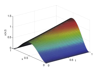
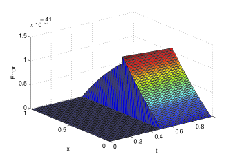
Fig. 1: The numerical behavior of the approximate solution (left) and absolute error (right) for Example 1.

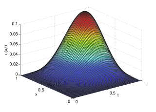
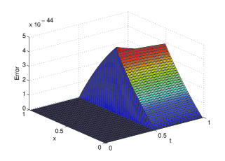
Fig. 2: The numerical behavior of the approximate solution (left) and absolute error (right) for Example 2.

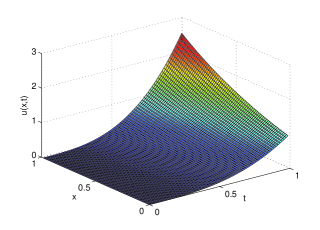
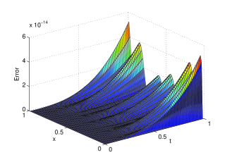
Fig. 3: The numerical behavior of the approximate solution (left) and absolute error (right) for Example 3.

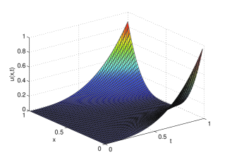
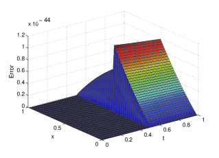
Fig. 4: The numerical behavior of the approximate solution (left) and absolute error (right) for Example 4.

6 Conclusion

In this paper, a new numerical method based on the CWs was proposed to obtain an approximate solution for the variable-order time fractional mobile-immobile advection-dispersion model. To this end, a new operational matrix of variable-order fractional derivative for the CWs was obtained and employed to obtain the approximate solution for the problem under study. Along the way a new family of piecewise functions was introduced and used to obtain a general approach for forming this matrix. In the proposed method, solution of the problem under consideration was expanded in terms of the the CWs. The operational matrix of variable-order fractional derivative and some properties of CWs were employed to transform its solution to the solution of a linear system of algebraic equations, which greatly simplified the problem as well as achieved a good approximate solution for it. Our proposed method is very efficient and convenient in solving such initial-boundary value problems because all the conditions are used. Also, the implementation of the proposed method is very simple for solution of the problem under consideration. The accuracy of the proposed method was shown for some examples, which shows that our proposed method is very accurate for the problem under study.

References

- [1] H. T. C. Pedro, M. H. Kobayashi, J. M. C. Pereira, and C. F. M. Coimbra, “Variable order modeling of diffusive convective effects on the oscillatory flow past a sphere,” J. Vib. Control, vol. 14, pp. 1569–1672, 2008.
- [2] L. E. S. Ramirez and C. F. M. Coimbra, “On the selection and meaning of variable order operators for dynamic modelling,” Int. J. Differ. Equ., vol. 2010, pp. 846107, 16 pp, 2010.
- [3] L. E. S. Ramirez and C. Coimbra, “On the variable order dynamics of the nonlinear wake caused by a sedimenting particle,” Physica D, vol. 240, pp. 1111–1118, 2011.
- [4] H. Sun, W. Chen, H. Wei, and Y. Chen, “A comparative study of constant-order and variable-order fractional models in characterizing memory property of systems,” Eur. Phys. J. Spec. Top., vol. 193, pp. 185–192, 2011.
- [5] J. J. Shyu, S. C. Pei, and C. H. Chan, “An iterative method for the design of variable fractional-order fir differintegrators,” Signal Process, vol. 89, pp. 320–327, 2009.
- [6] C. Coimbra, “Mechanics with variable-order differential operators,” Ann. Phys., vol. 12(11-12), pp. 692–703, 2003.
- [7] A. V. Chechkin, R. Gorenflo, and I. M. Sokolov, “Fractional diffusion in inhomogeneous media,” J. Phys. A: Math. Gen., vol. 38, pp. 679–684, 2005.
- [8] F. Santamaria, S. Wils, E. D. Schutter, and G. J. Augustine, “Anomalous diffusion in purkinje cell dendrites caused by spines,” Neuron, vol. 52, pp. 635–648, 2006.
- [9] H. G. Sun, W. Chen, and Y. Q. Chen, “Variable-order fractional differential operators in anomalous diffusion modeling,” Phys. A, vol. 388, pp. 4586–4592, 2009.
- [10] H. G. Sun, Y. Q. Chen, and W. Chen, “Randomorder fractional differential equation models,” Sign. Process., vol. 91, pp. 525–530, 2011.
- [11] S. Umarov and S. Steinberg, “Variable order differential equations and diffusion with changing modes,” Zeitschrift fr Analysis und ihre Anwendungen, vol. 28, pp. 431–450, 2009.
- [12] C. Lorenzo and T. Hartley, “Variable order and distributed order fractional operators,” Nonlinear Dyn., vol. 29, pp. 57–98, 2002.
- [13] Y. Liu, Z. Fang, H. Li, and S. He, “A mixed finite element method for a time-fractional fourth-order partial differential equation,” Appl. Math. Comput., vol. 243, pp. 703–717, 2014.
- [14] A. Atangana and D. Baleanu, “Numerical solution of a kind of fractional parabolic equations via two difference schemes,” Abstr. Appl. Anal., vol. 2013, pp. 828764,8, 2013.
- [15] M. M. Meerschaert and C. Tadjeran, “Finite difference approximations for fractional advection dispersion equations,” J. Comput. Appl. Math., vol. 172, pp. 65–77, 2004.
- [16] Y. Zhang, “A finite difference method for fractional partial differential equation,” Appl. Math. Comput., vol. 215, pp. 524–529, 2009.
- [17] C. Tadjeran, M. M. Meerschaert, and H. P. Scheffler, “A second order accurate numerical approximation for the fractional diffusion equation,” J. Comput. Phys., vol. 213, pp. 205–213, 2006.
- [18] R. Lin, F. Liu, V. Anh, and I. Turner, “Stability and convergence of a new explicit finite-difference approximation for the variable-order nonlinear fractional diffusion equation,” Applied Mathematics and Computation, vol. 212, pp. 435–445, 2009.
- [19] S. Shen, F. Liu, J. Chen, I. Turner, and V. Anh, “Numerical techniques for the variable order time fractional diffusion equation,” Applied Mathematics and Computation, vol. 218, pp. 10861–10870, 2012.
- [20] Y. Chen, L. Liu, B. Li, and Y. Sun, “Numerical solution for the variable order linear cable equation with bernstein polynomials,” Applied Mathematics and Computation, vol. 238, pp. 329–341, 2014.
- [21] M. G. . P. Manohar, “Matrix method for numerical solution of space-time fractional diffusion-wave equations with three space variables,” Afr. Mat., vol. 25, pp. 161–181, 2014.
- [22] N. H. Sweilam, M. M. Khader, and H. M. Almarwm, “Numerical studies for the variable-order nonlinear fractional wave equation,” Fractional Calculus and Applied Analysis, vol. 15, pp. 669–683, 2012.
- [23] H. Sun, W. Chen, C. Li, and Y. Chen, “Finite difference schemes for variable-order time fractional diffusion equation,” International Journal of Bifurcation and Chaos, vol. 22(4), p. 1250085 (16 pages), 2012.
- [24] P. Zhung, F. Liu, V. Anh, and I. Turner, “Numerical methods for the variable-order fractional advection-diffusion equation with a nonlinear source term,” SIAM J. NUMER. ANAL, vol. 47(3), pp. 1760–1781, 2009.
- [25] A. Atangana, “On the stability and convergence of the time-fractional variable order telegraph equation,” Journal of Computational Physics, vol. 293, pp. 104–114, 2015.
- [26] Y.-M. Chen, Y.-Q. Wei, D.-Y. Liu, and H. Yu, “Numerical solution for a class of nonlinear variable order fractional differential equations with legendre wavelets,” Applied Mathematics Letters, vol. 46, pp. 83–88, 2015.
- [27] V. A. P. Zhuang, F. Liu and I. Turner, “Numerical methods for the variable-order fractional advection-diffusion equation with a nonlinear source term,” Society for Industrial and Applied Mathematics, vol. 47(3), pp. 1760–1781, 2009.
- [28] M. H. Heydari, M. R. Hooshmandasl, and F. Mohammadi, “Legendre wavelets method for solving fractional partial differential equations with dirichlet boundary conditions,” Applied Mathematics and Computation, vol. 234, pp. 267–276, 2014.
- [29] M. Heydari, M. Hooshmandasl, G. Barid Loghmani, and C. Cattani, “Wavelets galerkin method for solving stochastic heat equation,” International Journal of Computer Mathematics, pp. 1–18, 2015.
- [30] M. Heydari, M. Hooshmandasl, F. M. Ghaini, and C. Cattani, “Wavelets method for the time fractional diffusion-wave equation,” Physics Letters A, vol. 379, no. 3, pp. 71–76, 2015.
- [31] M. H. Heydari, M. R. Hooshmandasl, F. Maalek Ghaini, and F. Fereidouni, “Two-dimensional Legendre wavelets for solving fractional poisson equation with dirichlet boundary conditions,” Engineering Analysis with Boundary Elements, vol. 37, pp. 1331–1338, 2013.
- [32] H. Zhang, F. Liu, M. S. Phanikumar, and M. M. Meerschaert, “A novel numerical method for the time variable fractional order mobile immobile advection dispersion model,” Computers and Mathematics with Applications, vol. 66, pp. 693–701, 2013.
- [33] M. Heydari, M. Hooshmandasl, and F. M. Ghaini, “A new approach of the Chebyshev wavelets method for partial differential equations with boundary conditions of the telegraph type,” Applied Mathematical Modelling, vol. 32, pp. 1597–1606, 2014.
- [34] M. Heydari, M. Hooshmandasl, F. Mohammadi, and C. Cattani, “Wavelets method for solving systems of nonlinear singular fractional volterra integro-differential equations,” Commun Nonlinear Sci Numer Simulat, vol. 19, pp. 37–48, 2014.
- [35] S. G. Hosseini and F. Mohammadi, “A new operational matrix of derivative for Chebyshev wavelets and its applications in solving ordinary differential equations with non analytic solution,” Appl. Math. Sci., vol. 5(51), pp. 2537–25448, 2011.