Dynamics of Solitons in the One-Dimensional Nonlinear Schrödinger Equation

Abstract

We investigate bright solitons in the one-dimensional Schrödinger equation in the framework of an extended variational approach. We apply the latter to the stationary ground state of the system as well as to coherent collisions between two or more solitons. Using coupled Gaussian trial wave functions, we demonstrate that the variational approach is a powerful method to calculate the soliton dynamics. This method has the advantage that it is computationally faster compared to numerically exact grid calculations. In addition, it goes far beyond the capability of analytical ground state solutions, because the variational approach provides the ability to treat excited solitons as well as dynamical interactions between different wave packets. To demonstrate the power of the variational approach, we calculate the stationary ground state of the soliton and compare it with the analytical solution showing the convergence to the exact solution. Furthermore, we extend our calculations to nonstationary solitons by investigating coherent collisions of several wave packets in both the low- and high-energy regime. Comparisons of the variational approach with numerically exact simulations on grids reveal excellent agreement in the high-energy regime while deviations can be observed for low energies.

1 Introduction

Solitons are nondispersive wave packets and they are commonly known to exist as a general phenomenon in nonlinear wave dynamics in various fields Eichler1 ; Eichler2 ; Tikhonenkov2008 ; Khaykovich2002 ; Strecker2002 ; Paredes2016 ; Anderson1985 ; Syafwan2012 . The fact that the wave packet keeps its shape arises from two counter-acting influences. A broadening effect is compensated by an attractive interaction, so that there is an intermediate state where the wave packet is stable. Beyond the existence of soliton wave packets in various systems their nonstationary dynamics is of high interest. This can e. g. be collective oscillations of slightly excited solitons or collisions between them.

In this paper, we focus on quantum mechanical solitons in Bose-Einstein condensates (BECs). Here, Heisenberg’s uncertainty principle, i. e. the kinetic energy term of the condensate, favors a broadening of the wave packet. By contrast, an attractive interaction, e. g. attractive s-wave scattering or an additional long-range interaction Wunner2008 , favors a shrinking condensate wave function. As a consequence, the BEC soliton exists when these terms compensate each other. In general, one distinguishes bright and dark solitons, where bright solitons exhibit an increased density resulting from attractive interactions while dark solitons are density minima due to repulsive interactions Pethick2008 .

Mathematically, the condensate wave function obeys the time-dependent Gross-Pitaevskii equation (GPE) Gross61a ; Pitaevskii61a ; Dalfovo1999 ; Ueda2010 , a nonlinear extension of the ordinary Schrödinger equation in which the nonlinear interaction term results from a mean-field approximation of the BEC. In general, several methods can be used to solve the GPE in order to determine the condensate’s ground state and its dynamics. These are e. g. the direct numerical integration in the one-dimensional case, the discretization of the wave function on a grid, as well as the description of the condensate within a variational approach Eichler1 ; Eichler2 ,

From the theoretical point of view, the one-dimensional BEC-soliton is of particular interest, because in this case the GPE can be solved analytically and the wave function of the condensate can be expressed by a simple analytic function Pethick2008 . This wave function, however, can only describe the ground state of the soliton, while dynamical solutions beyond a simple translation in space, excitations, or collisions are not accessible within this analytical approach. Thus, the latter situations require a different method and in this paper we describe a promising possibility using an extended variational approach based on coupled Gaussian wave functions. Such variational approaches have already been applied successfully to different questions arising in the field of BECs ranging from the simple reproduction of its ground state wave function Huepe2003 ; PerezGarcia1996 ; PerezGarcia1997 ; Yi2000 ; Yi2001 ; Parker2009 ; Muruganandam2012 , over issues of stability Kreibich2012 ; Kreibich2013a , ground and excited states of BECs with long-range $1/r$- or dipolar interactions Rau2010a ; Rau2010b ; Rau2010c , to the collapse dynamics of the condensate Huepe1999 ; Junginger2010 ; Junginger2012b ; junginger2012d ; Junginger2013b . However, in these situations a direct comparison between variational and directly numerical approaches has not been performed or has not been possible. Therefore, it is one of the goals of this paper to provide direct comparisons of these approaches.

In experiments, the BEC is usually confined in a harmonic trap whose ground state wave function is of pure Gaussian form. The choice of using Gaussian variational approaches is therefore straightforward in these cases. Regarding solitons in the absence of external traps, the situation is different, because the condensate wave function exhibits a broad heavy-tail distribution. As a consequence, it is a nontrivial question to what extent a Gaussian-based approach is capable of recovering the correct results. As we will demonstrate below, only few coupled Gaussians are necessary to obtain converged wave functions. In addition to the description of the condensate’s ground state, a particular advantage of the variational approach lies in its capability to derive equations of motion of the condensate dynamics analytically. This is due to the fact that its reduction of the degrees of freedom in general makes the computational effort significantly smaller – often by several orders of magnitude in the computation time as compared to grid calculations. Nevertheless, the accuracy of the variational approach is high enough to correctly describe the condensate dynamics. We demonstrate this for the collision of solitons, for which we directly compare the collision dynamics of the variational approach with that obtained from numerical grid calculations.

Our paper is organized as follows: In Sec. 2, we present the theoretical description of the solitons, review the analytical solution of the ground state, and introduce the variational approach. In Sec. 3, we demonstrate by comparison with numerically exact simulations, the capability of the variational approach to reproduce both the stationary as well as dynamical behavior of single and colliding solitons.

2 Theory

In mean-field approximation, the dynamics of one-dimensional BEC solitons with wave function $\psi$ is described by the time-dependent GPE

$$\textup{i}\hbar\frac{\mathrm{d}}{\mathrm{d}t}\psi(x,t)=\left[-\frac{\hbar^{2}}{2m}\frac{\mathrm{d}^{2}}{\mathrm{d}x^{2}}+g|\psi(x,t)|^{2}\right]\psi(x,t)\,.$$ (1)

Here, $m$ is the mass of the bosons and $g$ describes the scattering interaction between the single bosons within an s-wave approximation. Negative values of $g$ mean an attractive interaction while positive values describe a repulsive one. In this paper, we only consider the case $g<0$. Due to the absence of any external potential in Eq. (1), the particles are free in the $x$-direction and the total dynamics is determined by the counterplay between Heisenberg’s uncertainty principle (i. e. the kinetic energy term) and the attraction between the particles.

The free parameter $g<0$ in Eq. (1) suggests a different behavior of the underlying system in dependence of its actual value. However, using an appropriate system of units, this parameter can be eliminated from Eq. (1), showing that the underlying physics is the same for all $g<0$. To do so, we measure the action in units of $\hbar$ and the unit of mass is set to $m_{0}=2m$. Furthermore, the unit of energy is $E_{0}={\hbar^{2}}/({m_{0}x_{0}^{2}})$ with $x_{0}$ being the unit of length, and the coupling constant is measured in terms of $g_{0}={\hbar^{2}}/({m_{0}x_{0}})$. Since the unit of length, $x_{0}$, is a free parameter, its value and, thus, the value of $g_{0}$ can always be chosen such that one obtains $g=-1$ in the scaled units. Without loss of generality the GPE simplifies to

$$\textup{i}\frac{\mathrm{d}}{\mathrm{d}t}\psi(x,t)=\hat{H}\psi(x,t)$$ (2)

with the Hamiltonian

$$\hat{H}=-\frac{\mathrm{d}^{2}}{\mathrm{d}x^{2}}-|\psi(x,t)|^{2}\,.$$ (3)

2.1 Analytical solution of the soliton’s ground state

As mentioned in the introduction, the stationary case of the GPE (2) can be solved analytically. As one can find e. g. in the book of Pethick and Smith Pethick2008 , the ground state of the soliton is given by

$$\psi(x,t)=\frac{b}{\cosh(ax)}\,\mathrm{e}^{-\textup{i}\mu t}\,,$$ (4)

where $\mu<0$ is the chemical potential and the parameters $a$ and $b$ determine the width of the soliton and its amplitude through the relations

$$a^{2}=-\mu\quad\text{and}\quad b^{2}=-2\mu$$ (5)

with $\mu=-{1}/{16}$ for normalized wave functions. The mean-field energy of the soliton (4) is given by the expectation value

$$E=\left\langle-\frac{\mathrm{d}^{2}}{\mathrm{d}x^{2}}-\frac{1}{2}|\psi(x,t)|^{2}\right\rangle=-\frac{1}{48}\,,$$ (6)

where the additional factor $1/2$ is necessary in order to avoid a double-counting of the two-particle interactions. The negative value of the energy shows that the soliton is a bound state.

2.2 Lattice calculation

A straightforward way to obtain the time evolution in the excited case or if several solitons collide is to iterate the wave function on a spacial lattice. Therefore, we label the single lattice sites with the variable $j\in\mathbb{Z}$ and the distance between them with $\Delta x$. In order to obtain a time-dependent wave function of an excited soliton one then applies the time-evolution operator $U(t,t_{0})$ which reads

$$U(t_{0}+\delta t,t_{0})=1-\textup{i}\hat{H}\delta t+O(\delta t^{2})$$ (7)

for small time steps $\delta t$. Note that the first-order approximation of the time-evolution operator is not norm-conserving in general in contrast to, e. g., a Crank-Nicolson scheme numericalrecipes . However, using sufficiently small time steps $\delta t$, a possible error can be kept negligibly small which we verify in addition by a direct calculation of the time-dependence of the norm in our simulations. The value $\psi(x_{j},t_{0}+\delta t)$ of the wave function at the lattice site $j$ is then given by

$$\begin{split}\psi(x_{j},t_{0}+\delta t)&\approx\psi(x_{j},t_{0})\\ &+\textup{i}\left[\frac{\mathrm{d}^{2}}{\mathrm{d}x^{2}}+|\psi(x_{j},t_{0})|^{2}\right]\psi(x_{j},t_{0})\delta t\,\end{split}$$ (8)

and the second derivative therein can be evaluated via

$$\frac{\mathrm{d}^{2}}{\mathrm{d}x^{2}}\psi(x_{j},t_{0})=\frac{\psi(x_{j-1},t_{0})+\psi(x_{j+1},t_{0})-2\psi(x_{j},t_{0})}{\Delta x^{2}}\,.$$ (9)

With Eq. (8) one can calculate the wave function at any time, and we will use this method to compare the variational approach with numerically exact results.

2.3 Variational approach to the soliton

The purpose of this paper is to describe the one-dimensional soliton dynamics within a variational framework. In this approach, we parametrize the wave function

$$\psi(x,t)=\psi(x,\vec{z}(t))$$ (10)

by a set of complex and time-dependent variational parameters $\vec{z}(t)$. In order to determine the dynamics of the system, we use the McLachlan variational principle Frenkel1934 ; McLachlan1964

$$\|\textup{i}\dot{\psi}-\hat{H}\psi\|^{2}=\textup{min}\,.$$ (11)

If the wave function $\psi$ is an exact solution of the GPE (1), the norm in Eq. (11) vanishes and the minimum is zero, while it is nonzero for an approximate solution. The optimal time-evolution of the trial wave function is obtained by requiring a minimum norm meaning that the time-evolution of the variational wave function is solved with the least possible error. The application of the time-dependent variational principle (11) to Gaussian functions is well-established in the literature, so that we only briefly sketch the basic steps in the following. For a detailed description, we refer the reader to Refs. Rau2010a ; Rau2010b ; Rau2010c and references therein.

Calculating the minimum of Eq. (11) using the general approach (10) yields a set of first-order coupled differential equations

$$\Braket{\frac{\partial\psi}{\partial\vec{z}}}{\textup{i}\dot{\psi}+\frac{\mathrm{d}^{2}}{\mathrm{d}x^{2}}\psi+\left missing}{\psi}=0$$ (12)

which determine the time-evolution of the system. In addition, the energy of the system is given by the energy functional

$$E=\Braket{-\frac{\mathrm{d}^{2}}{\mathrm{d}x^{2}}-\frac{1}{2}\left missing}{\psi}{{}^{2}}\,.$$ (13)

For our investigations, we use as a trial wave function a superposition of Gaussians according to

$$\psi=\sum\limits_{n=1}^{{N_{\text{g}}}}g_{n}\quad\text{with}\quad g_{n}=\mathrm{e}^{-\alpha_{n}x^{2}+\beta_{n}x+\gamma_{n}}\,,$$ (14)

where ${N_{\text{g}}}$ is the number of Gaussians used to approximate the soliton(s). The parameter $\alpha_{n}$ determines the width of each Gaussian, $\gamma_{n}$ its weight and phase, and $\beta_{n}$ the velocity and position to the wave package. Altogether, the total set of variational parameters can be summarized by $\vec{z}=[\alpha_{1}$,$\beta_{1}$,$\gamma_{1},\ldots$,$\alpha_{{N_{\text{g}}}}$, $\beta_{{N_{\text{g}}}}$,$\gamma_{{N_{\text{g}}}}]^{\mathsf{T}}$ and we note that by initializing the single Gaussians $g_{n}$ with appropriate different linear coefficients $\beta_{n}$, also several spatially separated solitons can be described by the trial wave function (14). Evaluating the dynamical equations (12) for the trial wave function (14) yields after some calculation the equations of motion for the variational parameters

$$\dot{\alpha}_{n} =-4\textup{i}\alpha_{n}^{2}+\textup{i}V_{2}^{n},$$ (15a)

$$\dot{\beta}_{n} =-4\textup{i}\alpha_{n}\beta_{n}-\textup{i}V_{1}^{n},$$ (15b)

$$\dot{\gamma}_{n} =-2\textup{i}\alpha_{n}+\textup{i}\beta_{n}^{2}-\textup{i}V_{0}^{n}\,,$$ (15c)

where $V_{0}^{n},V_{1}^{n}$ and $V_{2}^{n}$ are solutions of the linear system of equations

$$\begin{split}\sum\limits_{n=1}^{{N_{\text{g}}}}\Braket{\frac{\partial\psi}{\partial\vec{z}}}{g_{n}\left(x^{2}V_{2}^{n}+xV_{1}^{n}+V_{0}^{n}\right)}=-\left\langle\frac{\partial\psi}{\partial\vec{z}}\bigg{|}|\psi|^{2}\psi\right\rangle&\,.\end{split}$$ (16)

Since the trial wave function $\psi$ is composed of Gaussian functions, all integrals occurring here are of the type $\int_{-\infty}^{\infty}x^{d}\,\mathrm{e}^{-\alpha x^{2}+\beta x+\gamma}\,\mathrm{d}x$ with $d=0,1,2,3,4$ and they are trivial to be calculated analytically.

In order to provide a better physical understanding, we note that the momentum $p_{n}$ and central position $x_{n}$ of each soliton are related to the variational parameters via

$$p_{n} =\text{Im}(\beta_{n})\,,$$ (17a)

$$x_{n} =\frac{\text{Re}(\beta_{n})}{2\alpha_{n}}\,.$$ (17b)

2.3.1 Single-Gaussian approximation to the soliton

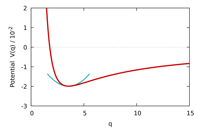
Figure 1: Potential $V(q)$, Eq. (18), of the Hamiltonian picture describing a one-dimensional soliton in the framework of a single Gaussian variational approach (red line). The minimum represents the stable ground state of the soliton and the oscillation frequency for small excitations can be obtained from the harmonic approximation (blue line).

From the equations of motion (15), one cannot easily see that the Gaussian approach is able to reproduce the soliton ground state. However, regarding the simplest approximation of a single soliton described by a single Gaussian wave function (${N_{\text{g}}}=1$), this is easily visible. For this purpose, we define the generalized coordinate $q=\sqrt{\left\langle x^{2}\right\rangle}=1/(2\sqrt{\text{Re}\,\alpha_{1}})$ and its conjugate momentum $p={\text{Im}\,\alpha_{1}}/{\sqrt{\text{Re}\,\alpha_{1}}}$. In this special case, the dynamical equations (15) and the energy functional (13) can be evaluated analytically and they are equivalent to Hamilton’s equations corresponding to the Hamiltonian

$$H(p,q)=T(p)+V(q)=p^{2}\;+\;\frac{1}{4q^{2}}-\frac{1}{4\sqrt{\pi}q}\,,$$ (18)

which defines a potential $V(q)$. As shown in Fig. 1, this potential exhibits a minimum (located at $q_{\textup{min}}=2\sqrt{\pi}$) which corresponds to the soliton’s ground state. The form of the potential $V(q)$ also shows that the soliton is stable with respect to small excitations, and a harmonic approximation of the potential at its minimum yields the collective oscillation frequency of the atomic cloud. In case of a description with a larger number of Gaussians, such a global Hamiltonian description is no longer possible, however this qualitative picture remains valid.

3 Results

3.1 Stationary solutions

We begin by discussing the stationary ground state of a single soliton. Due to the translational invariance of the system, it is appropriate to treat the system in its center of mass frame. In this case, the soliton’s center is located at $x=0$ and this also holds for all the coupled Gaussian wave functions, meaning that we can set $\beta_{n}=0$ throughout in this case. Stationary solutions within the variational approach are given if all the time-derivatives in Eq. (15) are zero [except the oscillating phase in Eq. (15c)]. The resulting equations then form a nonlinear system of equations for the variational parameters which we solve analytically for a single Gaussian ($N_{g}=1$) and numerically otherwise after providing appropriate initial values.

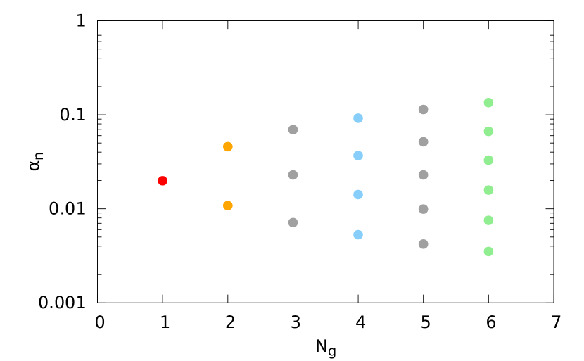
Figure 2: Variational parameters $\alpha_{n}$ for the stationary ground state of a single soliton described by different numbers ${N_{\text{g}}}$ of coupled Gaussians wave functions. For the ground state, all the width parameters are real and result in a purely real wave function as expected from the analytical solution (4). (The parameters $\gamma_{n}$ which determine the weight of each Gaussian are not shown here, and the colors of the dots for ${N_{\text{g}}}=1,2,4,6$ correspond to the line colors in Fig. 3.)

As the result of this root search, Fig. 2 shows the values of the variational width parameters $\alpha_{n}$ in dependence of the number ${N_{\text{g}}}$ of coupled Gaussian wave functions. The width parameters $\alpha_{n}$ of the trial wave function are all real in this case yielding a purely real ground state wave function as it is expected from the analytical solution (4). In addition to the width parameters, the root search also provides the values of the parameters $\gamma_{n}$ which determine the weight of each Gaussian (not shown). Using a single Gaussian $({N_{\text{g}}}=1)$, the value of $\alpha_{n}=1/(16\pi)$ is the best fit to the non-Gaussian soliton wave function (4). Adding a second, coupled Gaussian (${N_{\text{g}}}=2$), the tendency of the single contributions is that one of them corresponds to a larger width and the other to a smaller width. This trend continues with increasing number ${N_{\text{g}}}$ of Gaussians, i. e. the smallest (largest) width parameter becomes smaller (larger) and the others cover the intermediate regime.

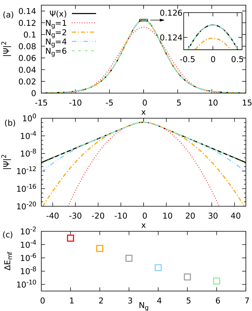
Figure 3: Comparison of the approximated wave functions within the variational approach (colored nonsolid lines) and the analytical solution (4) (black solid line). Panel (a) shows the wave function on a linear axis, illustrating the general behavior. In panel (b) a logarithmic scale is used in order to demonstrate the heavy-tail approximation behavior. Panel (c) shows the difference between the mean-field energy and the analytical ground state energy [$\Delta E_{\text{mf}}=E_{\text{mf}}+1/48$ according to Eq. (6)]. An additional Gaussian in the trial wave function improves the ground state energy by roughly one to two orders of magnitude.

In Fig. 3, we show the soliton wave functions which correspond to the width parameters from Fig. 2. The colored solid lines present the results of the variational approach and the dashed black line is the analytic result (4). As it becomes obvious in Fig. 3(a), a single Gaussian (${N_{\text{g}}}=1$; red line) qualitatively reproduces the correct soliton wave function, while it quantitatively fails to reproduce the higher density at the center of the soliton. A number of ${N_{\text{g}}}=2$ Gaussians (orange line) already improves the wave function significantly over the whole spacial range; the density peak compared with the pure Gaussian form is reproduced better and also the tendency of a more rapid decrease of the density away from the center is visible. For even higher number of Gaussians (${N_{\text{g}}}=4$; blue line and ${N_{\text{g}}}=6$; green line), the true wave function is approximated better and better and a difference to the variational approach is no longer visible within the linewidth of the plot [see the inset in Fig. 3(a)].

As we demonstrate in Fig. 3(b), this behavior not only holds at the center of the soliton but also for its tail: The pure Gaussian variational approach (${N_{\text{g}}}=1$) clearly fails to reproduce the heavy-tail density distribution of the soliton. This is clearly expected since the Gaussian trial wave function decays like $\exp(-x^{2})$ while the true soliton (4) only decays like $\exp(-x)$ for $x\to\infty$. Far away from the soliton’s center, the difference between the true and the trial wave function is, therefore, several orders of magnitude. Increasing the number of Gaussian, the tail-approximation soon becomes better with improvements of several orders of magnitude for each step of ${N_{\text{g}}}$. Finally, only ${N_{\text{g}}}=6$ coupled Gaussians are sufficient to reproduce the correct tail behavior over a very broad range.

The improvement of the wave function’s approximation with increasing number of coupled Gaussians is also reflected in the value of the mean-field energy which one obtains from the variational approach. To show this, we present in Fig. 3(c) the difference between the ground state energy within the variational approach and the value (6) of the analytical solution, $\Delta E_{\text{mf}}=E_{\text{mf}}+1/48$. For a single Gaussian, this difference is $\Delta E_{\text{mf}}=9.39\times 10^{-4}$, but it decreases by about one to two orders of magnitude with each additional Gaussian. For ${N_{\text{g}}}=6$ coupled Gaussian, the ground state energy is approximated very well with an error only of the order of $10^{-10}$. This, again, proves that the variational approach even with a low number of Gaussians is highly appropriate in order to approximate the soliton wave function.

3.2 Dynamics and collisions

As we have seen in Sec. 3.1 the variational approach converges rapidly to the analytical stationary bright soliton solution for increasing number of Gaussians. In this section, we address the question to what extent the variational approach is capable of describing the dynamics of the system. Therefore, we investigate the dynamics of collisions between several solitons in the following.

3.2.1 Collisions of two solitons

As a simple case, we first consider two colliding solitons. For this case, we use one and two Gaussians per soliton, and describe the collision in its center-of-mass frame. Under the assumption that the colliding solitons consist of the same number of particles, they both have the same momentum and the same distance to the origin of the center-of-mass frame,

$$x_{1}=-x_{2}\equiv x_{0}\,,$$ (19a)

$$p_{2}=-p_{1}\equiv p\,.$$ (19b)

For the initial soliton wave function, we take in the variational approach Eq. (14) with an appropriate set of variational parameters and for the grid calculations, we discretize the wave function of each individual soliton according to

$$\psi(x,t=0)=\sqrt{\frac{1}{8}}\,\frac{\mathrm{e}^{\textup{i}p(x-x_{0})+\textup{i}\varphi}}{\cosh[(x-x_{0})/4]}\,,$$ (20)

where $x_{0}$ is the central position of the soliton, and $p,\varphi$ are the initial momentum and phase, respectively. Configurations of several solitons can also be initialized by Eq. (20) if their overlap is negligible. The global phase of the solitons is a free parameter and not measurable. Only their relative phase matters which we take into account by setting the phase of the first soliton to zero, while introducing a phase shift $\Delta\varphi$ between the two solitons,

$$\varphi_{1} =0\,,$$ (21a)

$$\varphi_{2} =\Delta\varphi\,.$$ (21b)

By an appropriate choice of $\Delta\varphi$ the wave functions can be set, inter alia, symmetric ($\Delta\varphi=0$) or antisymmetric ($\Delta\varphi=\pi$). Note that the initial separation of the solitons needs to be chosen large enough so that the overlap of the solitons is negligible at the beginning. With these choices, the only remaining physical parameters in the soliton collisions are their phase difference $\Delta\varphi$ and their initial momentum $p$. In the numerical simulations, the number of Gaussians ${N_{\text{g}}}$ is a further computational input parameter.

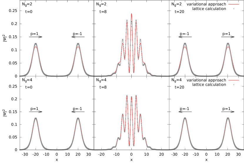
Figure 4: Collision of two solitons with initial momentum $|p|=1$ and phase difference $\Delta\varphi=0$. The comparison is shown between the results obtained with the variational approach (red lines) with ${N_{\text{g}}}=2$ (top row; one Gaussian per soliton) and ${N_{\text{g}}}=4$ (bottom row; two Gaussians per soliton) and the numerically exact dynamics (gray dots). The wave functions are plotted before ($t=0$), during ($t=8$), and after ($t=20$) the collision.

High-energy collisions

In Fig. 4, we consider the high-energy collision of two fast moving solitons, where we define ’fast’ with respect to the kinetic energy of the soliton in its center-of-mass frame, where it is $\langle p^{2}\rangle=\left\langle\psi|-\partial_{x}^{2}|\psi\right\rangle={1}/{48}$ with $\psi$ in Eq. (4). From this, we take

$$\bar{p}=\sqrt{\frac{1}{48}}\approx 0.144$$ (22)

as a reference for the magnitude of the soliton momentum and to classify a high- and low-energy regime of the dynamics. We compare the results obtained from the variational approach (red lines) and from numerically exact grid calculations (gray dots). For the initial momentum we set $p=1$ which is significantly larger than $\bar{p}$ in Eq. (22). The phase difference between the solitons is set to $\Delta\varphi=0$ which implies that the wave function is symmetric.

In the top row of Fig. 4 only a single Gaussian per soliton is used (red line; ${N_{\text{g}}}=2$ altogether). At $t=0$ both solitons are well separated in space so that their overlap can be neglected and they approach each other with the same momentum $p=1$, respectively. As we have already discussed in the stationary case, the simple variational approach qualitatively reproduces the exact soliton solution, but small quantitative differences are present. At time $t=8$ the solitons strongly overlap and interfere, resulting in several density peaks. It is clearly visible that both the variational approach as well as the numerically exact solution show the same behavior. After the collision ($t=20$; third column) the solitons move away from each other in the same state of motion as before the collision. Between the variational approach and the application of an approximative time-evolution operator, no differences in the shape and height of the solitons before and after the collision are visible, which shows that the latter is an appropriate method to integrate the dynamics.

We note that the computational effort to obtain these results shows significant differences between both approaches: The variational approach is about 75 times faster than the lattice calculation while still maintaining nearly the same quantitative behavior.

In the bottom row of Fig. 4, the same situation is shown using ${N_{\text{g}}}=4$ coupled Gaussians (two Gaussians per soliton). The improvement in the variational approach is evident. The collision dynamics in the variational framework and the numerically exact solution can no longer be distinguished although the variational approach is still five times faster than the lattice calculation. Even at the time of high spacial overlap, the variational approach perfectly reproduces the soliton wave functions. It is furthermore remarkable that, although there are ${N_{\text{g}}}=4$ Gaussian wave functions involved in the simulation process, they form two well-separated solitons also after their collision.

By increasing the initial momentum of the colliding solitons (not shown) the amount of peaks during the overlapping regime increases. Changing the phase difference between the solitons to a value different than $\Delta\varphi=0$ or $\Delta\varphi=\pi$ also the symmetry in the collision dynamics gets lost. However, the variational approach remains capable of describing the behavior correctly. . Fabcic2008a .

Low-energy collisions

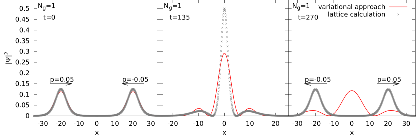
Figure 5: Collision of two solitons with initial momentum $|p|=0.05$ and phase difference $\Delta\varphi=0$. The dynamics for the variational approach (red line) was calculated for ${N_{\text{g}}}=2$ Gaussians (one Gaussian per soliton) and is compared with the results of the lattice calculations (gray dots).

We have seen that the variational approach is capable of describing the dynamics of the solitons correctly in the high-energy regime. Next we consider collisions where the momentum of the solitons is lower than their rest momentum $\bar{p}$. The collision of two solitons with a momentum of $p=0.05\ll\bar{p}$ is shown in Fig. 5. The phase difference between the solitons is set to $\Delta\varphi=0$ and the variational approach uses ${N_{\text{g}}}=2$ Gaussians (one Gaussian per soliton).

Since we are plotting the modulus squared of the wave function, there is no difference visible at $t=0$ between Figs. 4 and 5. At $t=135$, during the collision, the solitons overlap strongly and the wave function’s amplitude within the variational approach is significantly smaller than expected from the grid calculations. However, the general shape of the interfering solitons, i. e. the main peak at $x=0$ and two side maxima at $x\approx\pm 10$, is clearly reproduced by the variational approach. Significant differences between the two descriptions become obvious at $t=270$. Here, the grid calculation shows two well-separated, departing solitons. The solitons show the same behavior as they did during collusions with high momentum. By contrast, within the variational approach the wave packet has not yet separated into different solitons (red line). Instead, they have partially merged. It takes the solitons described by the variational approach another time span of $\Delta t=230$ to separate. After they have separated the solitons oscillate and their shape is not invariant any more (not shown in the figure). Note that during the whole simulation, the total energy as well as the norm of the wave function is conserved.

We have carefully checked that the observed merging effect also occurs when increassing the number of coupled Gaussians, so that it is not an artifact of an insufficient choice of the trial wave function. However, from the fact that the merge only occurs in the low-energy regime, we conclude that it is rather a numerical effect due to the closeness of the parameters in variational space. It is a well-known phenomenon in coupled Gaussian approaches that singularities in the dynamical equations (12) occur if two (nearly) identical Gaussians contribute to the total wave function. This is clearly the case for low-energy collisions where both position and velocity of the soliton are almost identical during the collision.

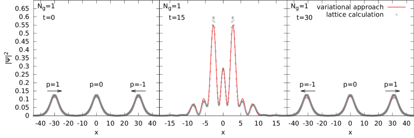
Figure 6: Collision of three solitons in the center-of-mass frame. Shown is the modulus squared of the wave function obtained from the variational approach with ${N_{\text{g}}}=6$ (red lines; two Gaussians per soliton) and the numerically exact dynamics (gray dots). The two moving solitons have the same momentum $p=\pm 1.5$ and there is no phase difference between them ($\Delta\varphi=0$).

3.2.2 Collision between several solitons

We have seen, that the variational approach produces excellent results for the collision of two solitons at high momentum. Next we consider the dynamics of three solitons where two moving solitons approach a soliton at rest. The moving solitons have the same momentum and accordingly hit the third soliton at the same time. We place the resting soliton in the center of coordinates so that we are again in the center-of-mass frame. Furthermore, the phase difference between the moving solitons is set to zero, so that the wave function is symmetric. In Fig. 6 the collision of three solitons is shown with the moving solitons initially having a momentum of $p=\pm 1.5$. The variational approach for ${N_{\text{g}}}=6$ (two Gaussians per soliton) is compared with the results of lattice calculations.

Before the collision (left frame) barely any difference between the variational approach and the lattice calculation is visible. This changes slightly during the collision (center frame). While the variational approach reproduces the shape of the lattice calculations very well in the surroundings of the two maxima, the maxima themselves slightly differ from the lattice calculations. The two moving solitons penetrate the one at rest and all three solitons are in the same state of movement as before (right frame). The small differences during the collision do not affect the behavior after it. As in the first frame, no differences between the variational approach and the lattice calculations are visible on the linear scale. This shows that the variational approach is capable of producing excellent agreement even for several soliton interactions.

Our simulations show that the Gaussian variational approach correctly describes collisions of even more solitons (not presented in this paper). For investigations of the corresponding dynamics for odd wave functions as well as animations, we refer the reader to Ref. ilg .

4 Conclusion

In this paper, we have investigated solitons in the one-dimensional GPE within an extended variational approach using coupled Gaussian wave functions. We have demonstrated that the variational approach perfectly reproduces the ground state of the soliton concerning the shape of the wave function as well as the ground state energy. This observation is especially remarkable because the soliton wave function differs from the pure Gaussian form with regard to its heavy-tail decay and the increased density at its center. The time-dependent variational approach applied in this paper also well describes the soliton dynamics in the high-energy regime. Already a small number of trial wave functions are sufficient to reproduce the time-dependent density distribution to a very high accuracy. By contrast, in the low-energy regime differences between the numerical and the variational approach can be observed which we expect to result from numerical issues due to the almost identical contribution of different wave functions during the low-energy collisions.

We note that the methods described in this paper are directly applicable to higher-dimensional systems with more complicated interactions Eichler1 ; Eichler2 and that our results agree with previous studies in similar cases using perturbation theory Michinel1999 . Our future work will also take into account the low-energy regime of slowly moving solitons in more detail involving Gaussian constraints in the dynamical equations Fabcic2008a .

References

- (1) R. Eichler, D. Zajec, P. Köberle, J. Main, G. Wunner, Phys. Rev. A 86, 053611 (2012)
- (2) R. Eichler, J. Main, G. Wunner, Phys. Rev. A 83, 053604 (2011)
- (3) I. Tikhonenkov, B.A. Malomed, A. Vardi, Phys. Rev. Lett. 100, 090406 (2008)
- (4) L. Khaykovich, F. Schreck, G. Ferrari, T. Bourdel, L.D.C. J. Cubizolles, Y. Castin, Science 296, 1290 (2002)
- (5) K.E. Strecker, G.B. Partridge, A.G. Truscott, R.G. Hulet, Nature 417, 150 (2002)
- (6) A. Paredes, H. Michinel, Physics of the Dark Universe 12, 50 (2016)
- (7) D. Anderson, M. Lisak, Phys. Rev. A 32, 2270 (1985)
- (8) M. Syafwan, H. Susanto, S.M. Cox, B.A. Malomed, J. Phys. A: Math. Theor. 45, 075207 (2012)
- (9) G. Wunner, H. Catarius, T. Fabčič, P. Köberle, J. Main, T. Schwidder, AIP Conf. Proc. 1076, 282 (2008)
- (10) C.J. Pethick, H. Smith, Bose-Einstein Condensation in Dilute Gases (Cambridge, 2008)
- (11) E.P. Gross, Il Nuovo Cimento 20, 454 (1961)
- (12) L.P. Pitaevskii, Soviet Physics JETP 13, 451 (1961)
- (13) F. Dalfovo, S. Giorgini, L. P. Pitaevskii, S. Stringari, Rev. Mod. Phys. 71, 463 (1999)
- (14) M. Ueda, Fundamentals and new frontiers of Bose-Einstein condensation (World Scientific Publishing Co. Pte. Ltd., Singapore, 2012)
- (15) C. Huepe, L.S. Tuckerman, S. Métens, M.E. Brachet, Phys. Rev. A 68, 023609 (2003)
- (16) V.M. Pérez-García, H. Michinel, J.I. Cirac, M. Lewenstein, P. Zoller, Phys. Rev. Lett. 77, 5320 (1996)
- (17) V.M. Pérez-García, H. Michinel, J.I. Cirac, M. Lewenstein, P. Zoller, Phys. Rev. A 56, 1424 (1997)
- (18) S. Yi, L. You, Phys. Rev. A 61, 041604 (2000)
- (19) S. Yi, L. You, Phys. Rev. A 63, 053607 (2001)
- (20) N.G. Parker, C. Ticknor, A.M. Martin, D.H.J. O’Dell, Phys. Rev. A 79, 013617 (2009)
- (21) P. Muruganandam, S.K. Adhikari, Laser Phys. 22, 813 (2012)
- (22) M. Kreibich, J. Main, G. Wunner, Phys. Rev. A 86, 013608 (2012)
- (23) M. Kreibich, J. Main, G. Wunner, J. Phys. B: At. Mol. Opt. Phys. 46, 045302 (2013)
- (24) S. Rau, J. Main, G. Wunner, Phys. Rev. A 82, 023610 (2010)
- (25) S. Rau, J. Main, H. Cartarius, P. Köberle, G. Wunner, Phys. Rev. A 82, 023611 (2010)
- (26) S. Rau, J. Main, P. Köberle, G. Wunner, Phys. Rev. A 81, 031605 (2010)
- (27) C. Huepe, S. Métens, G. Dewel, P. Borckmans, M.E. Brachet, Phys. Rev. Lett. 82, 1616 (1999)
- (28) A. Junginger, J. Main, G. Wunner, Phys. Rev. A 82, 023602 (2010)
- (29) A. Junginger, M. Dorwarth, J. Main, G. Wunner, J. Phys. A: Math. Theor. 45, 155202 (2012)
- (30) A. Junginger, J. Main, G. Wunner, T. Bartsch, Phys. Rev. A 86, 023632 (2012)
- (31) A. Junginger, M. Kreibich, J. Main, G. Wunner, Phys. Rev. A 88, 043617 (2013)
- (32) W.H. Press, ed., Numerical recipes: the art of scientific computing, 3rd edn. (Cambridge University Press, Cambridge [u.a.], 2007), ISBN 978-0-521-88068-8
- (33) J. Frenkel, Clarendon Press, Oxford (1934)
- (34) A.D. McLachlan, Molecular Physics, 8, 39 (1964)
- (35) T. Fabčič, J. Main, G. Wunner, J. Chem. Phys. 128, 044116 (2008)
- (36) T. Ilg, Bachelor thesis, Universität Stuttgart (2015), doi:10.18419/opus-8778
- (37) H. Michinel, V.M. Pérez-García, R. de la Fuente, Phys. Rev. A 60, 1513 (1999)