Scale invariant cosmology III: dynamical models and comparisons with observations

Abstract

Aims. We want to examine the properties of the scale invariant cosmological models, also making the specific hypothesis of the scale invariance of the empty space at large scales.

Methods. Numerical integrations of the cosmological equations for different values of the curvature parameter $k$ and of the density parameter $\Omega_{\mathrm{m}}$ are performed. We compare the dynamical properties of the models to the observations at different epochs.

Results. The main numerical data and graphical representations are given for models computed with different curvatures and density-parameters. The models with non-zero density start explosively with first a braking phase followed by a continuously accelerating expansion. The comparison of the models with the recent observations from supernovae SN Ia, BAO and CMB data from Planck 2015 shows that the scale invariant model with $k=0$ and $\Omega_{\mathrm{m}}=0.30$ very well fits the observations in the usual $\Omega_{\mathrm{m}}$ vs. $\Omega_{\Lambda}$ plane and consistently accounts for the accelerating expansion or dark energy.

The expansion history is compared to observations in the plot $H(z)$ vs. redshift $z$, the parameters $q_{0}$ is also examined, as well the recent data about the redshift $z_{\mathrm{trans}}$ of the transition between braking and acceleration. These dynamical tests are fully satisfied by the scale invariant models. The past evolution of matter and radiation density is studied, it shows small differences with respect to the standard case.

Conclusions. These first comparisons are encouraging further investigations on scale invariant cosmology with the assumption of scale invariance of the empty space at large scales.

1 Introduction

In the two previous papers of this series, we have derived the equations of a scale invariant cosmology and studied their properties. Two tentative, but fundamental, hypotheses are at the basis of these works. The first is that we may apply a general equation of the gravitational field, which in addition to the general covariance of General Relativity also possesses the property of scale invariance. Developments along this line were already performed in the past by Eddington (1923); Dirac (1973); Canuto et al. (1977). The second hypothesis is that the empty space, for exemple in the sense it is used in the Minkowski metric, should be scale invariant at macroscopic and large scales. It means that if, at such scales, we extend or contract the empty space, its properties are still the same. This hypothesis, which as far we know is new in this context, allows us to establish some differential equations connecting the scale factor $\lambda(x^{\mu})$ and the Einstein cosmological constant $\Lambda_{\mathrm{E}}$, this leads to relation (1). It also brings constraints on the scale factor and useful simplifications in the scale invariant equations.

The two above hypotheses lead to far-reaching consequences in physics and cosmology. The basic equations of cosmology are modified, showing an acceleration of the expansion after a certain initial period, the duration of which depends on the mean density of the Universe. Another major consequence of the scale invariance is that the laws of conservation of matter-energy show some dependence on the cosmic time. This dependence is very weak for models with a non-zero matter density, but at the conceptual level this is not a minor effect.

We do think it is worth to undertake the present exploration for two main reasons. One is that the recent cosmological results suggest that a totally unknown form of matter-energy, the dark energy, dominates the energy content of the Universe. This is a major problem. The other main reason is that scale invariance is not a kind of adjusted trick to make things work. But it is a basic physical change, that responds to the fundamental wish (Dirac 1973) that the equations expressing basic laws should be invariant under the widest group of transformations.

In this work, we construct the corresponding cosmological models, examine their dynamical properties and make close comparisons with observations. If there is no disagreement, this may be considered as encouraging, studies and comparisons will have to be pursued. If we find some serious disagreement, we may turn to the conclusion that at least one, or maybe the two fundamental hypotheses we have made do not correspond to the reality of Nature.

In Section 2, we express the equations of cosmology in an integrable form. In Section 3, we find and discuss the numerical solutions of the scale invariant models for the flat case with $k=0$, while the cases with the curvature parameter $k=\pm 1$ are analyzed in Section 4. Section 5 is devoted to the comparisons of models and observations, in particular the density parameters and the Hubble constant at present. In Section 6, we perform some dynamical tests at other epochs concerning the Hubble parameter $H(z)$ vs. $z$, the value of the deceleration parameter $q_{0}$ and the transition from braking to acceleration. In Section 7, the evolution of the matter and radiation densities, as well as the temperature over the ages are derived. Section 8 contains the conclusions.

2 Scale invariant cosmological models

Scale invariance is the invariance to a transformation of the line element like $ds^{\prime}\,=\,\lambda(x^{\mu})\,ds$, where $ds^{\prime}\,{}^{2}=g^{\prime}_{\mu\nu}\,dx^{\mu}\,dx^{\nu}$ is the line element in the framework of General Relativity, while $ds^{2}=g_{\mu\nu}\,dx^{\mu}\,dx^{\nu}$ is the line element in a more general framework where scale invariance is a property. The scale factor $\lambda$ only depends on the cosmic time in agreement with the Cosmological Principle. The scale invariance of the empty space at large scales implies a solution for $\lambda$ of the form

$$\lambda\,=\,\sqrt{\frac{3}{\Lambda_{\mathrm{E}}}}\,\frac{1}{c\,t}\,.$$ (1)

If we take $\lambda$ to be unity at the present cosmic time $t_{0}$, we get $\lambda\,=\,t_{0}/t$ and thus $\dot{\lambda}/\lambda=-1/t$. The constraint on the choice of the origin of $t$ will come from the chosen cosmological models. Origins at time $t_{\mathrm{in}}$ larger than 0 considerably reduce the amplitude of the variations of the scale factor $\lambda$ over the ages.

The basic equations of the scale invariant cosmology, that we derived from the above two fundamental hypotheses are according to Paper II,

$$\frac{8\,\pi G\varrho}{3}=\frac{k}{R^{2}}+\frac{\dot{R}^{2}}{R^{2}}+2\,\frac{\dot{R}\dot{\lambda}}{R\lambda}\,\;,$$ (2)

and

$$-8\,\pi Gp=\frac{k}{R^{2}}+2\frac{\ddot{R}}{R}+\frac{\dot{R^{2}}}{R^{2}}+4\frac{\dot{R}\dot{\lambda}}{R\lambda}\,\;.$$ (3)

The combination of these two equations leads to

$$-\frac{4\,\pi G}{3}\,(3p+\varrho)=\frac{\ddot{R}}{R}+\frac{\dot{R}\dot{\lambda}}{R\lambda}\,\,.$$ (4)

The gravitational constant $G$ is a true constant, $k$ is the curvature parameter ($0$ and $\pm 1$), $p$ and $\varrho$ are the pressure and density in the scale invariant system. In these equations, we have also explicitly accounted for the scale invariance of the empty space at large scales. Compared to the standard equations of Friedman models, the above ones only differ by the presence of a term in $\dot{R}\,\dot{\lambda}/(R\,\lambda)$, which represents an acceleration opposed to gravitation, since $\dot{\lambda}/\lambda$ is negative, as seen above.

The solutions of these equations depend on the equation of state of the medium we are considering. For an equation of state of the form

$$P\,=\,w\,\varrho\,,\quad(\mathrm{with\;}c^{2}=1)\,,$$ (5)

where $w$ is a constant, the first two equations lead to a first integral

$$\varrho\,R^{3(w+1)}\,\lambda^{(3w+1)}\,=const.$$ (6)

as shown in Paper II. For the case $w=0$ of ordinary matter of density $\varrho_{\mathrm{m}}$, exerting no pressure, we get $\varrho_{\mathrm{m}}\,\lambda\,R^{3}=const.$ If $\lambda(t)$ is a constant, one gets the usual equations of cosmologies for the expansion term $R(t)$. In Section 7, we also consider the phase of the Universe evolution where radiation is dominating.

We are first searching the solution of the cosmological equations for the case of ordinary matter with density $\varrho_{\mathrm{m}}$ and $w=0$. We start from (2) and multiply it by $R^{3}\lambda$ so that we may use the above first integral of the equation of state,

$$\frac{8\,\pi G\varrho_{\mathrm{m}}R^{3}\lambda}{3}=k\,R\lambda+\dot{R}^{2}R\lambda+2\,\dot{R}R^{2}\dot{\lambda}\,$$ (7)

The first member is a constant. With $\lambda=t_{0}/t$ and choosing the timescale such that at present $t_{0}=1$, we have

$$\dot{R}^{2}R\,t-2\,\dot{R}\,R^{2}+k\,R\,t-C\,t^{2}=0\,,$$ (8)

with

$$C=\frac{8\,\pi G\varrho_{\mathrm{m}}\,R^{3}\lambda}{3}\,.$$ (9)

Eq. (8) is a differential equation of order 1 and degree 2. The time $t$ is expressed in units of the present time $t_{0}$ taken equal to 1, at which we also assume $R_{0}=1$. The origin, the Big-Bang if any one, occurs when $R(t)=0$ at an initial time $t_{\mathrm{in}}$ which is not necessarily 0. Indeed, the cosmological models below will show that it is only in the case of an empty Universe (cf. Paper II), that the origin appears to lie at $t_{\mathrm{in}}=0$. We notice that if we have a solution $R$ vs. $t$, then $(x\,R)$ vs. $(x\,t)$ is also a solution, thus the solutions are also scale invariant, as expected from our initial assumptions. To integrate this equation, we need to have numerical values of $C$, corresponding to different values of the density in the model Universe. The way of treating the problem depends on the curvature parameter $k$.

3 Cosmological models with a flat space ($k=0$)

The case of the Euclidean space is evidently the most interesting one in view of the confirmed results of the space missions investigating the Cosmic Microwave Background (CMB) radiation with Boomerang (de Bernardis et al. 2000), WMAP (Bennett et al. 2003) and the Planck Collaboration et al. (2015). Expression (8) becomes

$$\dot{R}^{2}R\,t-2\,\dot{R}\,R^{2}-C\,t^{2}=0\,,$$ (10)

In $t_{0}=1$ and $R_{0}=1$, with the Hubble constant at the present time $H_{0}=\dot{R_{0}}/R_{0}$, the above relation leads to

$$H^{2}_{0}-2\,H_{0}=C\,.$$ (11)

This allows us to express $H_{0}$ as a function of $C$ with

$$H_{0}\,=\,1\pm\sqrt{1+C},$$ (12)

where we take the sign + since $H_{0}$ is always positive.

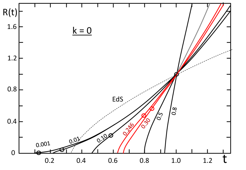
Figure 1: Some solutions of R(t) for the models with $k=0$ and $\Omega^{*}_{\mathrm{m}}=1$. The curves are labeled by the values of $\Omega_{\mathrm{m}}$, the usual density parameter defined by (14) and considered at the present time $t_{0}$. The Einstein-de Sitter model (EdS) is indicated by a dotted line. The small circles on the curves show the transition point between braking $(q>0)$ and acceleration $(q<0)$, for $\Omega_{\mathrm{m}}=0.80$, this point is at $R=2.52$. The two red curves indicate models corresponding to the observational values of $\Omega_{\mathrm{m}}=0.246$ (Frieman et al. 2008) and of $\Omega_{\mathrm{m}}=0.30$ given by the Planck Collaboration et al. (2015).

We now want to relate $C$ to the density parameters. For $k=0$, the critical matter density $\varrho^{*}_{\mathrm{c}}$ at time $t$ is obtained from (2) and the corresponding density parameter $\Omega^{*}_{\mathrm{m}}$ is defined by

$$\varrho^{*}_{\mathrm{c}}=\frac{3\,H^{2}}{8\pi G}\left(1-\frac{2}{t\,H}\right)\quad\mathrm{and}\;\quad\Omega^{*}_{\mathrm{m}}=\frac{\varrho_{\mathrm{m}}}{\varrho^{*}_{\mathrm{c}}}\,,$$ (13)

as studied in paper II. A remark about the notations: we put a * to the critical density and $\Omega$-parameter defined by (13) to distinguish them from the usual definitions of these parameters, which are

$$\varrho_{\mathrm{c}}=\frac{3\,H^{2}}{8\pi G}\,\;\;\quad\mathrm{and}\quad\Omega_{\mathrm{m}}=\frac{\varrho_{\mathrm{m}}}{\varrho_{\mathrm{c}}}\,.$$ (14)

We have the following relation between these two $\Omega$-parameters

$$\Omega_{\mathrm{m}}\,=\,\Omega^{*}_{\mathrm{m}}\left(1-\frac{2}{t\,H}\right)\,.$$ (15)

The term $\Omega_{\mathrm{m}}$ satisfies at all times the fundamental relation,

$$\Omega_{\mathrm{m}}\,+\,\Omega_{\mathrm{k}}\,+\Omega_{\lambda}=\,1\,\quad\mathrm{with}\quad\Omega_{\lambda}=\frac{2}{H\,t}\,,$$ (16)

and $\Omega_{\mathrm{k}}=-\frac{k}{H^{2}\,R^{2}}$, which is zero here. For $k=0$, we have $\Omega^{*}_{\mathrm{m}}=1$ at all times, according to (15) and (16). We have seen in Paper II that except for of $\Omega^{*}_{\mathrm{m}}=1$ and $\Omega_{\mathrm{k}}=0$ in the case where $k=0$, the various $\Omega$-parameters vary with time in scale invariant models. These parameters are generally considered at the present time (as is also the case in the $\Lambda$CDM models). This will be the practice generally adopted here, unless explicitly specified.

It is convenient to express $C$ (which determines the solution) as a function of parameter $\Omega_{\mathrm{m}}$. From (16), we have $\Omega_{\mathrm{m}}=1-\frac{2}{H_{0}}$ at the present time $t_{0}=1$, thus

$$H_{0}\,=\,\frac{2}{1-\Omega_{\mathrm{m}}}\,.$$ (17)

This expression gives $H_{0}$ (in unit of $t_{0}$) directly from $\Omega_{\mathrm{m}}$. We may also now obtain $C$ as a function of $\Omega_{\mathrm{m}}$ at time $t_{0}$ with the help of (11),

$$C=\frac{4}{(1-\Omega_{\mathrm{m}})^{2}}-\frac{4}{(1-\Omega_{\mathrm{m}})}=\frac{4\,\Omega_{\mathrm{m}}}{(1-\Omega_{\mathrm{m}})^{2}}\,,$$ (18)

a relation which allows us to integrate (10) for a chosen value of the density parameter $\Omega_{\mathrm{m}}$ at present.

Table 1: Cosmological parameters of some models with $k=0$ and different $\Omega_{\mathrm{m}}<1$, $\Omega_{\mathrm{m}}$ being the usual density parameter at present time $t_{0}$. Note that $\Omega^{*}_{\mathrm{m}}=1$ for all these models. $H_{0}(t_{0})$ is the values of the Hubble constant taking $t_{0}=1$, $t_{\mathrm{in}}$ is the time when $R(t)=0$, $\tau=t_{0}-t_{\mathrm{in}}$ is the age of the Universe in units where $t_{0}=1$, $\tau$(Gyr) is the age of the Universe in Gyr for the considered model assuming that the age of the model with $\Omega_{\mathrm{m}}=0.30$ is 13.8 Gyr, $H_{0}(\tau)$ is the Hubble constant in the unit of $\tau$, $t$(q=0) and $R$(q=0) are the values of $t$ and $R$ at the inflexion point, “$H_{0}$ obs“ is the value of the Hubble constant in km s^-1 Mpc^-1 for an age of the Universe equal to 13.8 Gyr (Frieman et al. 2008).

$\Omega_{\mathrm{m}}(t_{0})$	$C$	$H_{0}(t_{0})$	$t_{\mathrm{in}}$	$q_{0}$	$\tau$	$\tau$(Gyr)	$H_{0}(\tau)$	$t$(q=0)	$R$(q=0)	$\Omega_{\lambda}$	$H_{0}$ obs
0.001	0.0040	2.0020	0.0999	- 0.499	0.9001	37.6	1.802	0.126	0.010	0.999	127.7
0.010	0.0408	2.0202	0.2154	-0.490	0.7846	32.7	1.585	0.271	0.047	0.990	112.3
0.100	0.4938	2.2222	0.4641	- 0.400	0.5359	22.4	1.191	0.585	0.231	0.900	84.4
0.180	1.0708	2.4390	0.5645	- 0.320	0.4355	18.2	1.062	0.711	0.364	0.820	75.3
0.246	1.7308	2.6525	0.6265	- 0.254	0.3735	15.6	0.991	0.789	0.474	0.754	70.2
0.300	2.4490	2.8571	0.6694	-0.200	0.3306	13.8	.945	0.843	0.568	0.700	67.0
0.400	4.4444	3.3333	0.7367	-0.100	0.2633	11.0	0.878	0.928	0.763	0.600	62.2
0.500	8.0000	4.0000	0.7936	0.000	0.2064	8.6	0.826	1.000	1.000	0.500	58.5
0.800	80	10	0.9282	0.300	0.0718	3.0	0.718	1.170	2.520	0.200	50.9
0.990	39600	200	0.9967	0.490	.00335	0.14	0.669	1.256	21.40	0.010	47.4

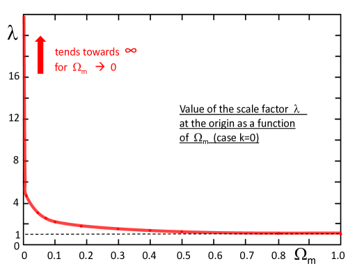
Figure 2: Values of the scale factor $\lambda$ at the origin $R(t)=0$ for models with $k=0$ and different density parameters $\Omega_{\mathrm{m}}$ at $t_{0}$. This curve shows that for increasing densities, the amplitude of the variations of the scale factors $\lambda$ is very much reduced.

While in the Friedman models, there is a unique value of the density $\varrho_{\mathrm{c}}$ corresponding to a flat space with $k=0$, the scale invariant cosmology permits a variety of the density parameter $\Omega_{\mathrm{m}}$ (14) at present for the flat space with $k=0$. This is a most interesting property, especially in view of the results of the CMB which support a flat Universe (de Bernardis et al. 2000; Bennett et al. 2003; Planck Collaboration et al. 2015). However, we have seen in Paper II that for $k=0$ the parameter $\Omega_{\mathrm{m}}$ is necessarily smaller than 1, since $\Omega_{\lambda}>0$ and (16) must be satisfied. Expression (18) shows that for $\Omega_{\mathrm{m}}$ ranging from $0\rightarrow 1$, $C$ covers the range from $0$ to infinity.

To integrate (10) numerically, we choose a present value for $\Omega_{\mathrm{m}}$, which determines $C$ according to (18) and we proceed to the integration backwards and forwards in time starting from the present chosen values $t_{0}=1$ and $R_{0}=1$. The integration provides $R(t)$, its derivatives and the related parameter $H$ and $q$. Fig. 1 shows some curves of $R(t)$ for different $\Omega_{\mathrm{m}}<1$, all these curves have $k=0$ and $\Omega^{*}_{\mathrm{m}}=1$. Table 1 provides some model data. The value of $H_{0}$ is given in a scale where $t_{0}=1$ (column 3), it is also given (column 8) in a scale where the time unit is the age of the Universe $\tau=t_{0}-t_{\mathrm{in}}$, while the last column gives the the value of $H_{0}$ in the current units [km s^-1 Mpc^-1]. To obtain $H_{0}$ in these units, we need to have an estimate of th age of the Universe. Frieman et al. (2008) give an estimate of 13.9 $\pm 0.6$ Gyr in a so-called consensus model and 13.8 $\pm 0.2$ Gyr in a fiducial model. Freedman & Madore (2010) provide an age estimate of 13.7 $\pm 0.5$ Gyr based on three different methods. The last column of the Table gives the value of $H_{0}$ expressed in usual units [km s^-1 Mpc^-1] for an adopted age $\tau$ of 13.8 Gyr. This value of the age of the Universe is also used in column 7 for obtaining the ages in Gyr.

In practice to get $H_{0}$ in [km s^-1 Mpc^-1], we proceed in the following way. The inverse of the age of 13.8 Gyr is $2.2683\cdot 10^{-18}$ s^-1, which in the units currently used for the Hubble constant is equal to 70.86 [km s^-1 Mpc^-1]. Thus, this is the value of $H_{0}$ that exactly corresponds to $H_{0}(\tau)=1.000$ in column 8 of Table 1. On the basis of this correspondence, we now multiply all values of $H_{0}(\tau)$ of column 8 by 70.86 [km s^-1 Mpc^-1] to get the values of $H_{0}$ in the last column. We see that $H_{0}=67$ [km s^-1 Mpc^-1] is the Hubble constant predicted for $\Omega_{\mathrm{m}}=0.30$ in agreement with Planck Collaboration et al. (2015). The fact that a good agreement is obtained for $\Omega_{\mathrm{m}}=0.30$ indicates that the expansion rate is correctly predicted by the scale invariant models in a consistent way with the age of the Universe.

From Table 1 and Fig. 1, we note the following properties of the scale invariant models with $k=0$ :

1. After an initial phase of braking, there is an acceleration of the expansion, which goes on all the way.

2. The differences of the expansion functions $R(t)$ with that of the classical Einstein-de Sitter model (thin broken line in Fig. 1) are large.

3. No curve $R(t)$ starts with an horizontal tangent, except the case of zero density which goes like $R(t)\sim t^{2}$ (Paper II).

4. All models with matter start explosively with very high values of $H={\dot{R}}/R$ and a positive value of $q$, indicating braking.

5. The higher the input density parameter $\Omega_{\mathrm{m}}$, the longer the initial braking phase. The locations of the inflexion points where $q$ changes sign are indicated for the models of different $\Omega_{\mathrm{m}}$ by a small open circle in Fig. 1, see also Table 1.

6. The lower the density, the longer the present age $\tau=t_{0}-t_{\mathrm{in}}$ of the models. This is also true for the ages given in Gyr.

7. The properties of the scale factor $\lambda$ deserve some comments. First, we recall that the behavior of $\lambda(t)$ derives from the assumption of the scale invariance of the empty space at macroscopic and large scales. For a totally empty space with $\varrho_{\mathrm{m}}=0$, the factor $\lambda$ would vary between $\infty$ at the origin, to 1 at present and to zero in an infinite future, as shown by the empty model in Paper II. Fig. 2 shows that as soon as matter becomes present the amplitude of the $\lambda$-variations falls dramatically. For example, for a present $\Omega_{\mathrm{m}}=0.30$, $\lambda$ varies only from 1.4938 to 1.0 between the origin and the present. Thus, the presence of about 1 H-atom by cubic meter on the average is sufficient to shift the initial $\lambda$ value from infinity to about 1.5. For $\Omega_{\mathrm{m}}$ tending towards unity, the scale factor $\lambda$ tends towards a constant equal to 1. Thus, the domain of $\lambda$-values is consistently determined by the matter content or in other words by the departures from the scale invariant empty space.

   

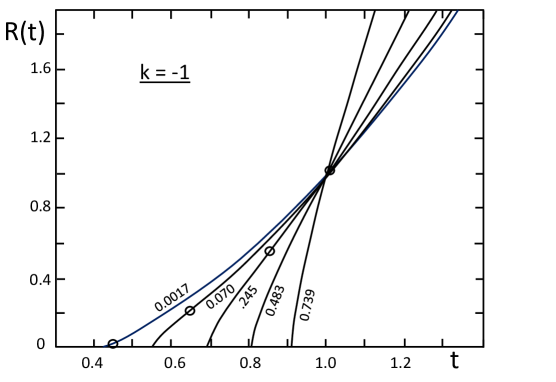
   Figure 3: Some solutions of $R(t)$ fro the models with $k=-1$. The curves are labeled by the values of $\Omega_{\mathrm{m}}$ at $t_{0}$, the usual density parameter defined by (14). The corresponding values of $\Omega^{*}_{\mathrm{m}}$ used to define $C$ are 0.001, 0.315, 0.70, 0.90, 0.98 from left to right.

8. The expressions of $q$ are different for the scale invariant and the $\Lambda$CDM models. For the flat scale invariant models, $q$ is given at all times by

   $$q=\frac{1}{2}-\Omega_{\lambda}\,,$$ (19)

   while for the flat $\Lambda$CDM models, it is

   $$q\,=\,\frac{1}{2}\Omega_{\mathrm{m}}-\Omega_{\Lambda}\,.$$ (20)

   The transition from braking to acceleration occurs, for the flat scale invariant case, when one has the equality $\Omega_{\mathrm{m}}=\Omega_{\lambda}=1/2$ at the transition, while in the $\Lambda$CDM model, it occurs when $\Omega_{\Lambda}=(1/2)\,\Omega_{\mathrm{m}}$, which gives a transition for $\Omega_{\mathrm{m}}=2/3$.

9. For the flat models with $\Omega_{\mathrm{m}}=0.30$, the values of the deceleration parameter $q_{0}$ at the present time are $q_{0}=-0.20$ for the scale invariant model and $q_{0}=-0.55$ for the $\Lambda$CDM model. The present acceleration is slightly stronger in the $\Lambda$CDM than in the corresponding scale invariant model.

10. We note the different behaviors of $H_{0}$ in unit of $t_{0}=1$ and in unit of $\tau$, the present age of the Universe. The Hubble constant $H_{0}$ expressed as a function of the age $\tau$ is smaller for higher densities, the same trend is noted for $H_{0}$ expressed in usual units [km s^-1 Mpc^-1]. The particular value $H_{0}=1/\tau$ is obtained for $\Omega_{\mathrm{m}}\simeq 0.24$ and $\Omega_{\lambda}\simeq 0.76$ for $k=0$.

11. As shown by Table 1, for the present $\Omega_{\mathrm{m}}=0.99$, $C$ is equal to 39600 and the model starting at $t_{\mathrm{in}}=0.99664$ nearly has a vertical expansion $R(t)$. This suggests that for $\Omega_{\mathrm{m}}=1$ the model inflates explosively all the way since the orgin. Whether this has some implications at the origin is an open question.

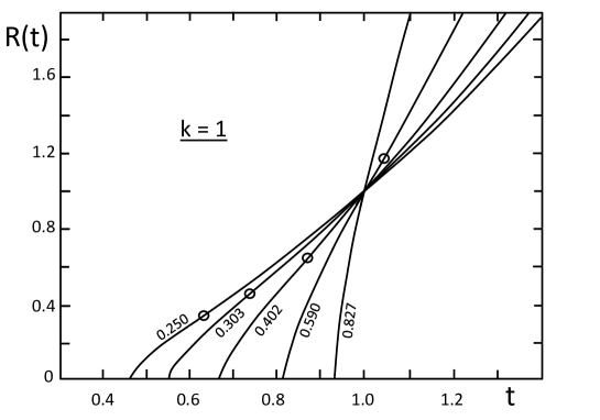
Figure 4: Some solutions of $R(t)$ for $k=+1$. The corresponding values of the usual density parameter $\Omega_{\mathrm{m}}$ at $t_{0}$ are indicated. The values of $\Omega^{*}_{\mathrm{m}}$ used to define the $C$-values are 1000, 3.0 , 1.5, 1.10, 1.01.

Below in Table (3), we provide the details of the relation $R(t)$ vs. time $t/t_{0}$, for the density parameter $\Omega_{\mathrm{m}}=0.30$, well supported by the Planck Collaboration et al. (2015). In this table, we also give the redshifts, the corresponding ages, Hubble parameters and scale factors.

Table 2: Cosmological parameters of some models with $k=-1$ and $k=+1$ for different values of the density parameter $\Omega^{*}_{\mathrm{m}}$ at time $t_{0}$. The usual density parameter at $t_{0}$ is $\Omega_{\mathrm{m}}$ in column 8. See also the remarks for Table 1.

$\Omega^{*}_{\mathrm{m}}$	$C$	$H_{0}(t_{0})$	$t_{\mathrm{in}}$	$q_{0}$	$\tau$	$H_{0}(\tau)$	$\Omega_{\mathrm{m}}$	$t$(q=0)	$R$(q=0)	$\Omega_{\lambda}$	$\Omega_{\mathrm{k}}$	$H_{0}$ obs
	k=-1
0.001	0.0010	2.4146	.4157	-.414	.5843	1.411	.0002	0.424	0.009	.828	0.172	100.0
0.100	0.1111	2.4530	.4701	-.398	.5299	1.300	.019	0.531	0.104	.815	0.166	92.1
0.315	0.4599	2.5684	.5467	-.355	.4533	1.164	.070	0.646	0.224	.779	0.152	82.5
0.500	1.0000	2.7320	.6095	-.299	.3905	1.067	.134	0.734	0.342	.732	0.134	75.6
0.700	2.3333	3.0817	.6887	-.202	.3113	0.959	.246	0.843	0.536	.649	0.105	68.0
0.900	9.0000	4.3166	.8091	0.010	.1909	0.824	.483	1.006	1.028	.463	0.054	58.4
0.98	49	8.1414	.9090	0.247	.0910	0.741	.739	1.142	2.076	.246	0.015	52.5
0.999	999	32.639	.9791	0.438	.0209	0.682	.938	1.233	6.158	.061	0.001	48.3
	k=1
1.001	1001	32.639	.9791	0.439	.0209	0.682	.940	1.234	6.180	.061	-.001	48.3
1.010	101	11.050	.9356	0.323	.0644	0.712	.827	1.182	2.764	.181	-.008	50.4
1.100	11	4.3166	.8157	0.064	.1843	0.796	.590	1.042	1.179	.463	-.054	56.4
1.5	3	2.7321	.6679	-.164	.3321	0.907	.402	0.872	0.657	.732	-.134	64.3
2.0	2	2.4142	.6021	-.243	.3979	0.961	.343	0.797	0.534	.828	-.172	68.1
3.0	1.5	2.2247	.5475	-.298	.4525	1.007	.303	0.736	0.455	.899	-.202	71.3
10.0	1.1111	2.0541	.4819	-.355	.5181	1.064	.263	0.662	0.379	.974	-.237	75.4
1000	1.0001	2.0005	.4564	-.375	.5436	1.088	.250	0.634	0.354	1.00	-.250	77.0

4 The elliptic and hyperbolic scale invariant models

Although the non-Euclidean models are not supported by the observations of the CMB radiation (Planck Collaboration et al. 2015), we briefly present the main properties of these models. We first have to relate the constant $C$ to the density parameters. Expressing $C$ with (8) and (13), we get at time $t_{0}$

$$C=\frac{8\,\pi\,G\varrho_{\mathrm{m}}}{3}=\Omega^{*}_{\mathrm{m}}\,H^{2}_{0}\,\left(1-\frac{2}{t_{0}H_{0}}\right)\,,$$ (21)

and with (15)

$$\mathrm{and}\quad C\,=\,\Omega_{\mathrm{m}}\,H^{2}_{0}\,.$$ (22)

We see that the real density $\varrho_{\mathrm{m}}$ at the present time behaves like $C$ and thus as $\Omega_{\mathrm{m}}\,H^{2}_{0}$. From the basic equation (2) and the definition (13) of the critical density $\varrho^{*}_{\mathrm{c}}$, we also have the following relation between the geometrical parameter $k$ and $\Omega^{*}_{\mathrm{m}}$ at the present time,

$$\frac{k}{R^{2}_{0}}=H^{2}_{0}\left[(\Omega^{*}_{\mathrm{m}}-1)\left(1-\frac{2}{t_{0}H_{0}}\right)\right]\,,$$ (23)

which was relation (40) of Paper II. It allows us to eliminate $[1-2/(t_{0}\,H_{0})]$ from (21) and obtain

$$C\,=\,\frac{k\,\Omega^{*}_{\mathrm{m}}}{\Omega^{*}_{\mathrm{m}}-1}\,,\quad\mathrm{with}\;\;k=\pm 1\,.$$ (24)

A model is defined by its $\Omega^{*}_{\mathrm{m}}$-value at the present time. For integrating equation (8), we first choose an arbitrary value of $\Omega^{*}_{\mathrm{m}}$ for the considered $k$ and then use (24) to obtain the corresponding $C$–value. The integration of (8) from the present $t_{0}=1$ and $R_{0}=1$ is performed forwards and backwards to obtain $R(t)$ and its first and second derivatives. The value of $H_{0}=(\dot{R}/R)_{0}$ at the present time gives us the $\Omega_{\mathrm{m}}$-value corresponding to the chosen $\Omega^{*}_{\mathrm{m}}$, according to relation (15).

Here, for non zero curvature models, $\Omega_{\mathrm{m}}\neq(1-\Omega_{\lambda})$ at all times and we do not have $\Omega^{*}_{\mathrm{m}}$ equal to 1 as for $k=0$. $\Omega_{\mathrm{m}}$, $\Omega_{\mathrm{k}}$ and $\Omega_{\lambda}$, as well as $\Omega^{*}_{\mathrm{m}}$ vary with time in these models. We have seen in Sect. 4.1 of Paper II, that for $k=-1$, the variety of scale invariant models is necessarily restricted to those with $\Omega_{\mathrm{m}}<1$. For $k=1$, we found that if the condition $(\Omega_{\mathrm{k}}+\Omega_{\lambda})>0$ is satisfied, the variety of models is also restricted to those with $\Omega_{\mathrm{m}}<1$. From Table 2, we see that this condition is satisfied, this is why both sets of models with $k=\pm 1$ have the usual density parameter $\Omega_{\mathrm{m}}<1$.

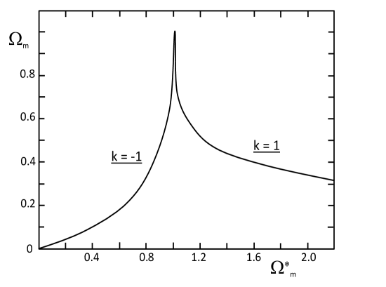
Figure 5: Relation between the two density parameters defined by (13) and (14) at time $t_{0}$. $\Omega_{\mathrm{m}}$ is the usual density parameter at present. For large values of $\Omega^{*}_{\mathrm{m}}$, the values of of $\Omega_{\mathrm{m}}$ tend towards an asymptotic limit of 0.25.

Figs. 3 and 4 illustrate some solutions for $k=\pm 1$ and Table 2 gives some model parameters for different values of $\Omega_{\mathrm{m}}$. From these figures, we see that the three families of $R(t)$ curves for $k=0$ and $k=\pm 1$ are on the whole not so different from each other. The curves for $k=\pm 1$ also show the same succession with first a braking and then an acceleration phase. For lower $\Omega_{\mathrm{m}}$, the initial expansion is less steep and starts earlier, while for $\Omega_{\mathrm{m}}$ approaching 1 the expansion tends to become explosive, as already seen for $k=0$. The relative similarity of the three families of curves indicates that the curvature term $k$ has a limited effect compared to the density (expressed by $C$ in the equations) and to the acceleration resulting from scale invariance. Unlike the Friedman models, the same density parameters $\Omega_{\mathrm{m}}$ may exist for different curvatures.

As for models with $k=0$, the models with $k=\pm 1$ may have all possible values of $C$, and thus of $\varrho_{\mathrm{m}}$, from 0 to infinity. However, they all have the usual density parameter $\Omega_{\mathrm{m}}$ smaller than 1.0, as mentioned above. For $k=-1$, the two density parameters $\Omega_{\mathrm{m}}$ and $\Omega^{*}_{\mathrm{m}}$ cover the range from 0 to 1, which is not particular. However, for $k=+1$, the behavior of the parameters is peculiar, as illustrated by Table 2. When $C$ increases from 1 to infinity, $\varrho$ increases from a minimum value to infinity. At the same time, $\Omega^{*}_{\mathrm{m}}$ decreases from infinity to 1.0, while $\Omega_{\mathrm{m}}$ goes from a limit of 0.25 to 1.0.

Fig. 5 illustrates the relation between the two density parameters at $t_{0}$, $\Omega_{\mathrm{m}}=\Omega^{*}_{\mathrm{m}}[1-2/(t_{0}\,H_{0})]$. For $k=-1$, $\Omega_{\mathrm{m}}$ grows first much slower than $\Omega^{*}_{\mathrm{m}}$ due to the subtraction of the term $2/(t_{0}\,H_{0})$. Then as $H_{0}$ becomes very large, $\Omega_{\mathrm{m}}$ grows fast. For $k=1$, as $\Omega^{*}_{\mathrm{m}}$ increases we have the opposite for the usual density parameter, this results from the fact that the term $[1-2/(t_{0}\,H_{0})]$ becomes very small. As an example from Table 2, for $\Omega^{*}_{\mathrm{m}}=1000$, $H_{0}=2.00050$, so that the term $[1-2/(t_{0}\,H_{0})]=0.00025$ and $\Omega_{\mathrm{m}}=0.25$. In all comparisons with observations, we will evidently use the $\Omega_{\mathrm{m}}$-parameter.

5 Comparisons of models and observations: the density parameters and the Hubble constant at present

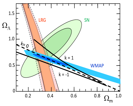
Figure 6: The constraints on $\Omega_{\Lambda}$ vs. the present $\Omega_{\mathrm{m}}$ from the observational data collected by Reid et al. (2010), with the constraints from WMAP5, from the Union SN sample and from the halo density field of luminous red galaxies of the SDSS DR7 as analyzed by Reid et al. (2010). We have superposed the results of the scale invariant models for $\Omega_{\lambda}$ and $\Omega_{\mathrm{m}}$ (at $t_{0}$) from Tables 1 and 2 for the different curvature parameters $k$.

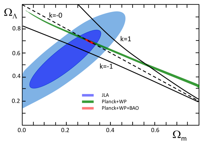
Figure 7: The $\Omega_{\Lambda}$ vs. the usual $\Omega_{\mathrm{m}}$ from the observational data collected by Betoule et al. (2014), cf. their Fig. 15. The SN sample from JLA (blue) is superposed with the Planck temperature and WMAP polarization measurements (green). The most stringent constraint (red) accounts for the BAO results. We have superposed the scale invariant model results for $\Omega_{\lambda}$ and $\Omega_{\mathrm{m}}$ from Tables 1 and 2 for the different curvature parameters.

Comparisons with observations are essential to invalidate or validate theories. In this section, we make comparisons for several important properties, in particular the density parameters and the expansion rate $H_{0}$.

5.1 The $\Omega$–parameters

Since the discovery of the acceleration of the expansion, a number of constraints on the $\Omega$–parameters have been found and analyzed in recent major works. The studies of the CMB with Boomerang (de Bernardis et al. 2000), WMAP (Bennett et al. 2003) and the Planck Collaboration et al. (2015) support more and more the flatness $k=0$ of the Universe. For example, the last Planck results (Planck Collaboration et al. 2015) give a value $\Omega_{\mathrm{k}}=0.00\pm 0.005$ at a 95% confidence limit. Over recent years, the various surveys globally converge towards similar results within always more stringent limits.

Frieman et al. (2008) found average values of $\Omega_{\mathrm{m}}=0.246\pm 0.028$ and $\Omega_{\Lambda}=0.757\pm 0.021$, their reference study was based on the magnitude-redshift data for supernovae, the CMB radiation measured by WMAP, the age constraints and the baryon acoustic oscillations (BAO). In this technique, one considers that the initial oscillations in the CMB, with a lengthscale defined by the sound velocity in the plasma, influence the clustering of galaxies and provide a reference length scale (150 Mpc), which is used to measure the cosmic distances and probe the acceleration of expansion. The analysis of the BAO from a sample of 893’319 galaxies in the Sloan Digital Sky Survey (SDSS) Data Release 7 (DR7) by Percival et al. (2010) leads to a slightly higher density ($\Omega_{\mathrm{m}}=0.286\pm 0.018$). Reid et al. (2010) examine the constraints from the clustering of luminous red galaxies in the SDSS DR7. The power spectrum of the halo density field of galaxies is sensitive to the dark matter density $\Omega_{\Lambda}$. Combining their data with WMAP 5 years results, they find $\Omega_{\mathrm{m}}=0.289\pm 0.019$, ($\Omega_{\Lambda}$ is here the complement to an $\Omega$-sum of 1.011$\pm 0.009$).

Clusters of galaxies provide another interesting constraint on the density parameters (Allen et al. 2011). Let $f_{\mathrm{gas}}$ be the ratio of the mass in the form of X-ray emitting gas to the total mass in clusters. This ratio in the largest concentrations of mass in the Universe is generally assumed constant and about equal to the baryon fraction. The assumption of a constant $f_{\mathrm{gas}}$ with redshift $z$ places constraints on the cosmological models. Combining these constraint with those of the CMB and supernovae leads to $\Omega_{\mathrm{m}}=0.275\pm 0.015$ and $\Omega_{\Lambda}=0.725\pm 0.016$. A recent study by Betoule et al. (2014) of the cosmological parameters with the project Joint Light-curve Analysis (JLA) combines the supernova results of two major surveys the SDSS and SNLS (SN Legacy Survey) together with the CMB data from Planck and WMAP, including also the constraints from BAO. This study gives very stringent conditions as illustrated by Fig. 7 and favors a value $\Omega_{\mathrm{m}}=0.295\pm 0.034$ .

Fig. 6 based on the results by Reid et al. (2010) and Fig. 7 based on the recent and very constraining results by Betoule et al. (2014) show the comparison of the observed density parameters $\Omega_{\mathrm{m}}$ and $\Omega_{\Lambda}$ with the results of our models. In the scale invariant models, $\Omega_{\lambda}$ represents the contribution of the effects of scale invariance to the energy-density. The flat model with $k=0$ and $\Omega_{\mathrm{m}}\approx 0.30$ remarkably well fits the various constraints. The two sets of models with non-zero curvature do not agree with observations, particularly the models with $k=1$.

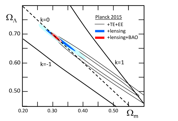
Figure 8: Data from Fig. 26 in Planck Collaboration et al. (2015): the black contours are from the various Planck spectra. The account of the lensing effect on temperature and polarization tightens the permitted domain (blue contours). The inclusion of both lensing and BAO constraints dramatically restrains the permitted domain (red contours). The thick black lines show the scale invariant model results as in Fig. 7.

The successive releases of CMB data from Boomerang, WMAP and Planck more and more constrain the density parameters. The Planck data particularly when combined with the BAO tightens very much the permitted interval for the $\Omega$-values. The Planck results (Planck Collaboration et al. 2015) support $\Omega_{\mathrm{m}}=0.308\pm 0.012$ in a flat model Universe. Fig. 8 compares these last results with the various models. We notice the strongly constrained red zone and its perfect agreement with the $k=0$ scale invariant models for the above value of $\Omega_{\mathrm{m}}$.

This confirms that a scale invariant model correctly account for the observed matter density and acceleration of the expansion, or in other words for the amount of the supposed dark matter. Thus, as far as the density parameters are concerned, the scale invariant cosmology shows agreement with observations. These results are encouraging to pursue the exploration of the consequences of the scale invariant cosmology.

5.2 The Hubble constant $H_{0}$ in relation with the $\Omega$-parameters

Another important test concerns the value of the Hubble constant at the present time $H_{0}$. The models internally provide the Hubble constant $H_{0}(\tau)$ as a function of the present age $\tau$ of the Universe (e.g. column 8 in Table 1). As seen above to get the value of $H_{0}$ in [km s^-1 Mpc^-1] from the models, we need both the present expansion rate $H_{0}(\tau)$ given by the models and an estimate of the present age of the Universe. In Tables 1 and 2, we have adopted an age of 13.8 Gyr consistent with the best present estimates and to derive the $H_{0}$-values corresponding to different parameters we proceed as explained in Sect. 3.

There has always been scatter in the results for $H_{0}$, this is still the case at present, although it is now much decreasing. Frieman et al. (2008) give a value $H_{0}=72\pm 5$ in [km s^-1 Mpc^-1], $73\pm 4$ is obtained by Freedman & Madore (2010), $68.2\pm 2.2$ by Percival et al. (2010), $69.4\pm 1.6$ by Reid et al. (2010), $70.2\pm 1.4$ by Allen et al. (2011), $67.8\pm 0.9$ by the Planck Collaboration et al. (2015).

The models in Table 1 for $k=0$ show the dependence of $H_{0}$ on the matter density. $H_{0}$ expressed in current units consistently decreases for an increasing matter density, since braking is more efficient. For values between $\Omega_{\mathrm{m}}=0.246$ and 0.308 corresponding to the values given by Frieman et al. (2008) and the Planck Collaboration et al. (2015), we get values of $H_{0}$ between 70.2 and 66.5 [km s^-1 Mpc^-1], a range very consistent with the observed one. If we would have adopted an age of 13.7 Gyr, these values would have been 67.0 and 70.7 and for an age of 13.9 Gyr, 66.0 and 69.7 respectively, values which would not change the conclusions.

Fig. 9 present the constraints on the $H_{0}$ values vs. the density parameter $\Omega_{\mathrm{m}}$ derived from the CMB, SN and clustering of LRG within the CDM models with free curvature and a constant $w$-parameter (Reid et al. 2010). Such a comparison is testing whether the present expansion rate $\dot{R}(t_{0})/R(t_{0})$ predicted by the models for the observed matter density $\Omega_{\mathrm{m}}$ is consistent with observations.

We see that the curve defined by the $k=0$ models nicely fits the central red zone, best constrained by the WMAP5 data together and the results from the clustering. The scale invariant models with $k=-1$ are not so much different from those with $k=0$, while the models with $k=1$ do not agree with the observational constraints. We may also do the comparison with the recent Planck data. For a matter density of $\Omega_{\mathrm{m}}=0.308\pm 0.012$, a value of $H_{0}=67.8\pm 0.9$ [km s^-1 Mpc^-1] is obtained in the $\Lambda$CDM model by the Planck collaboration. The scale invariant model with $k=0$ gives for the above density 66.5 $\pm 0.7$. Thus, we note that the agreement for the constraints set by $H_{0}$ vs. matter density is quite good.

Fig. 10 compares models and data from the Planck Collaboration et al. (2015) in the $\Omega_{\mathrm{k}}$ vs. $H_{0}$ plot. We verify that the models with $k=0$ perfectly cross the region defined by the Planck and BAO constraints, for a value $H_{0}$ very well corresponding to the Planck results. In this plot, the models with $k=\pm 1$ strongly diverge from observations.

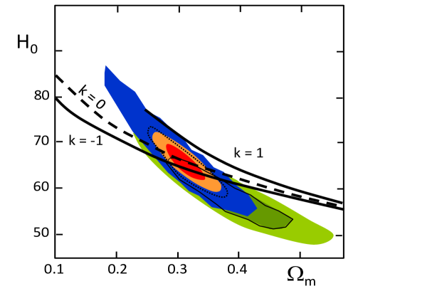
Figure 9: Observational data from Fig. 10 by Reid et al. (2010). The green contours represents the constraints from WMAP+SN, the blue from WMAP5+luminous red galaxies (LRG), the orange and red from WMAP5+SN+LRG in the $\Lambda$CDM models with free curvature and constant $w$-parameter for the equation of state. The scale invariant models of Table 1 and 2 with different curvature are over-plotted (black lines).

On the whole, the scale invariant cosmological models give in Table 1 a value of the Hubble constant $H_{0}$ in agreement with observation for $\Omega_{\mathrm{m}}=0.30$. The plots of $H_{0}$ vs. the density parameters $\Omega_{\mathrm{m}}$ and $\Omega_{\mathrm{k}}$ show an excellent agreement for a scale invariant model with $k=0$ and $\Omega_{\mathrm{m}}\approx 0.30$.

The tests we have made above concern the model properties at the present time. We have performed comparisons of the predictions of the scale invariant models with the recent observational constraints from the SN Ia, the BAO oscillations and CMB data concerning the energy-density parameters $\Omega_{\mathrm{m}}$, $\Omega_{\mathrm{k}}$ and $\Omega_{\Lambda}$, we have also examined the present expansion rate $H_{0}$ and its relation to the energy-density parameters. We now turn to some tests concerning different epochs in the evolution of the Universe.

6 Observational dynamical tests at other epochs

A major prediction of the cosmological models, including the scale invariant models, concerns the expansion history $R(t)$ of the Universe. The results depend on the basic equations with the conservation laws implied by the model equations. The tests we now perform concern past epochs in the history of the Universe. Several observational tests on the past dynamics of the Universe were successfully developed over the last decades. We may mention among others:

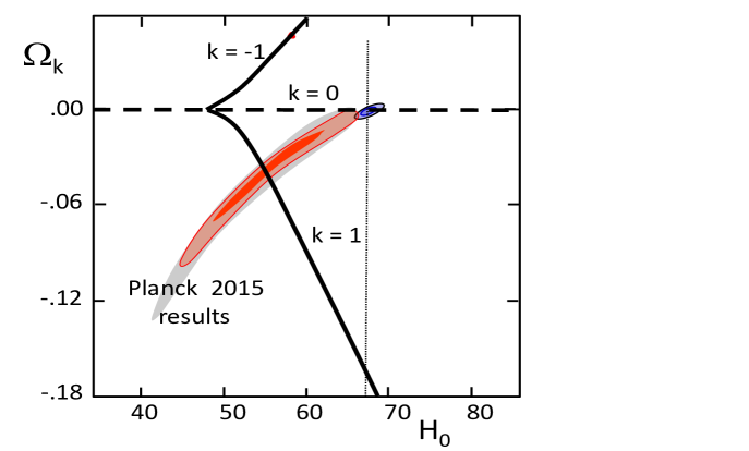
Figure 10: Data from Fig. 26 in Planck Collaboration et al. (2015), the gray zone only uses the TT spectra and polarization data, the red zone applies all spectra and polarization results, while the blue accounts in addition for the BAO constraints. The scale invariant models with different curvature $k$ are shown by thick black lines.

- The Hubble or magnitude-redshit (m-z) diagram based on distant supernovae of type Ia used as standard candles (Riess et al. 1998; Perlmutter et al. 1999).

- The preferred length-scale given by BAO provides a standard of length at large distances. The BAO may be observed in large galaxy and quasar surveys (Eisenstein et al. 2005).

- In the case of a very large survey, the preferred scale from BAO and large clusters may be studied in both the radial and tangential directions under the assumption that the observed objects are isotropic. This method first devised by Alcock & Paczynski (1979) allows one to test cosmological models, giving for example indications on both the angular distance and on the expansion rate $H(z)$ at the considered redshift, see also Blake et al. (2012); Busca et al. (2013).

- The method of ”cosmic chronometers” is based on the simple relation

$$H(z)=-\frac{1}{1+z}\,\frac{dz}{dt}\,,$$ (25)

obtained from $R_{0}/R=1+z$ and the definition of $H=\dot{R}/R$. The critical ratio $dz/dt$ is estimated from of a sample of passive galaxies (with ideally no active star formation) of different redshifts and age estimates (Jimenez & Loeb 2002; Simon et al. 2005; Melia & McClintock 2015; Moresco 2015).

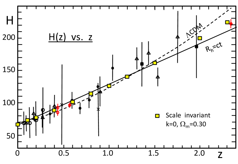
Figure 11: The $H(z)$ vs. redshift plot, with $H$ in km s^-1 Mpc^-1. The observations are the model-independent data collected by Melia & McClintock (2015). The black square are from Moresco (2015), the open circles from Zhang et al. (2014), the black circles from Moresco et al. (2012), the crosses by Stern et al. (2010), the open triangles from Simon et al. (2005). Three other recent model independent and high precision data are added as red points.The filled red point at z=2.34 is from the BAO data of the BOSS DR11 quasars by Delubac et al. (2015), the filled red point at z=0.57 is from the BAO given by clustering of galaxies in the BOSS from SDSS-III by Anderson et al. (2014), the two open and connected red points at z=0.43 represent one sample from an analysis by Moresco et al. (2016) of data from BOSS DR9 interpreted with two different sets of models of spectral evolution. The curves for the $\Lambda$CDM and $R_{h}=c\,t$ models are by Melia & McClintock (2015). The yellow squares indicate the predictions of the scale invariant model for $k=0$ and $\Omega_{\mathrm{m}}=0.30$.

6.1 The expansion history of the Universe

The determination of the expansion rate $H(z)$ vs. redshift represents a direct and constraining test on the expansion function $R(t)$ over the ages. In order to perform valid tests of the cosmological models, it is essential that the observational data are independent on the cosmological models, otherwise the results may be biased towards the used model. The method of the cosmic chronometer appears as a powerful one, since there is no assumption depending on a particular cosmological model, as emphasized by several authors, namely Simon et al. (2005); Stern et al. (2010); Melia & McClintock (2015); Moresco (2015); Moresco et al. (2016). In several cases, as pointed out by Melia & McClintock (2015), ”cosmological observations” based solely on BAO may have some dependence on the tested cosmology. We note, however, that the method of cosmic chronometers, although independent on the cosmological models, depends on the models of spectral evolution of galaxies, which are mainly based on the theory of stellar evoluton. This illustrates the well known fact that all cosmological tests have their weak and strong points.

Table 3 shows many properties of the scale invariant model with $k=0$ and $\Omega_{\mathrm{m}}=0.30$ as functions of redshift $z$. Column 7 gives the Hubble values $H(z)$ for different redshifts. These values of $H(z)$ are derived in the same way as for Table 1. To perform comparisons between models and observations, we use the data by Simon et al. (2005); Stern et al. (2010); Moresco et al. (2012); Zhang et al. (2014); Moresco (2015) as collected by Melia & McClintock (2015), completed by other recent high precision and model independent data (shown in red colour) by Anderson et al. (2014); Delubac et al. (2015); Moresco et al. (2016). Fig. 11 presents these data with different symbols according to the authors. The two connected open red circles at $z=0.43$ concern the same BAO at $z=0.43$, but where the ages are based on two different models of evolving passive galaxies (Moresco et al. 2016). We see that, at least here, the differences due to different models of stellar populations are rather limited. In this figure, we have also reported the $\Lambda$CDM model and a model where $R(t)$ linearly increases with time like the horizon $R_{h}=c\,t$ (Melia & McClintock 2015). According to these authors, this last model is better supported by different observations as suggested by several statistical tests they performed, a claim challenged by Moresco et al. (2016). Without entering this particular debate, we remark the significant differences between these two models at high $z$. In this context, we mention that Delubac et al. (2015) find a 2.5 $\sigma$ difference of the BAO at $z=2.34$ with the predictions of a flat $\Lambda$CDM model with the best-fit Planck parameters.

Interestingly enough, the scale invariant $k=0$ and $\Omega_{\mathrm{m}}=0.30$ model is intermediate between the $\Lambda$CDM and $R_{h}=c\,t$ models and it matches well the observations of the expansion history $H(z)$ vs. $z$ from cosmic chronometers. In particular, we notice the good agreement with the high precision data by Delubac et al. (2015).

6.2 The values of $q_{0}$ in the $\Lambda$CDM and scale invariant models

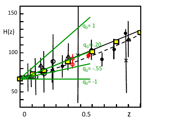
Figure 12: The lower left part of Fig. 11 with the lines indicating the slope $(dH/dz)_{0}$ for 4 different $q_{0}$-values. The value $q_{0}=-0.55$ corresponds to the flat $\Lambda$CDM, while $q_{0}=-0.20$ for the flat scale invariant model. For both models, a value $\Omega_{\mathrm{m}}=0.30$ is assumed.

The so-called deceleration parameter $q_{0}$ is testing the second derivative of $R(t)$ at $t_{0}$, thus it depends on the change of the expansion rate $H$ over the recent time, i.e. on the values of $H(z)$ over small redshifts $z$. As seen in Sect. 3, the $\Lambda$CDM and the scale invariant models predict different values of the deceleration parameter $q_{0}$. For $k=0$ and $\Omega_{\mathrm{m}}=0.30$, these are respectively -0.55 and -0.20, both corresponding to an acceleration, slightly stronger for the $\Lambda$CDM model. The parameter $q$ expresses a second derivative of $R(t)$ and is thus related to $dH/dz$, which we have studied in Fig. 11. We have

$$q=-\frac{\ddot{R}R}{\dot{R}^{2}}=-\frac{dH}{dt}\frac{R^{2}}{\dot{R}^{2}}-1=-\frac{dH}{dz}\frac{dz}{dt}\frac{1}{H^{2}}-1\,.$$ (26)

In the limit $z\rightarrow 0$, we have $-dz/dt=H_{0}$, thus we get

$$\left(\frac{dH}{dz}\right)_{0}=\,(q_{0}+1)H_{0}\,,$$ (27)

which relates $q_{0}$ and the derivative $(dH/dz)_{0}$ at the present time.

Fig. 12 shows the slopes $(dH/dz)_{0}$ for four different $q_{0}$-values, $q_{0}=1,-0.20,-0.55,-1.0$. These slopes have to be considered in the zone near the origin $z=0$, in view of the approximations we have made. The differences between the various slopes are significant. For a strongly decelerating Universe with $q_{0}=1$, we consistently see that the expansion factor $H$ was much larger in the past, thus the steeper slope in the figure. Conversely, for a moderately accelerating Universe the difference between past and present values is smaller. We remark that both the $\Lambda$CDM and scale invariant models for $\Omega_{\mathrm{m}}=0.30$ are within the scatter of the observations, so that it would be meaningless to speculate which one is the best. At this stage, we may conclude that the scale invariant model shows no disagreement with observations. Maybe higher precision data may allow a separation in the future.

6.3 The transition from braking to acceleration

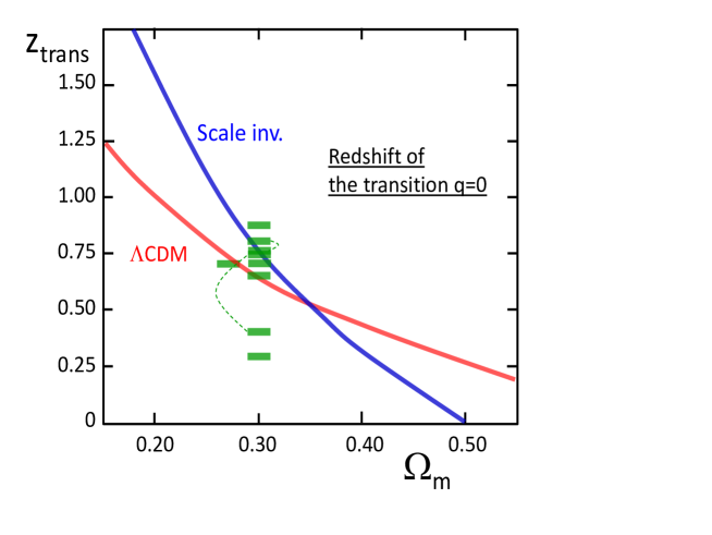
Figure 13: Relation between the redshift of the transition from the braking to the acceleration of expansion vs. the matter density $\Omega_{\mathrm{m}}$ for the flat $\Lambda$CDM and scale invariant models. The observational values discussed in the text are shown by small green rectangles.

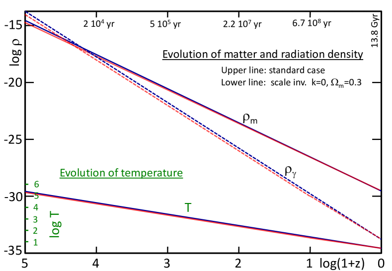
Figure 14: Evolution of matter density, radiation density and temperature as a function of redshift $z$. For each of the three quantities $\rho_{\mathrm{m}}$, $\rho_{\gamma}$ and $T$, the upper blue line corresponds to the standard case with the classical conservation laws, while the lower red line corresponds to the scale invariant solutions. For temperature, the two lines are very close to each other and cannot be distinguished in the Figure. On the upper side of the frame, the corresponding ages $t(z)-t_{\mathrm{in}}$ given by the flat scale invariant model with $\Omega_{\mathrm{m}}=0.30$ are indicated.

We have seen in Sect. 3 the conditions for the occurrence of the transition from braking to acceleration which produces an inflexion point in the expansion $R(t)$. For the scale invariant model with $k=0$, $q=0$ occurs when $\Omega_{\lambda}=\Omega_{\mathrm{m}}=\frac{1}{2}$. For $\Omega_{\mathrm{m}}=0.30$, the transition occurs at $R/R_{0}=0.568$ (cf. Table 1) corresponding to a transition redshift $z_{\mathrm{trans}}=0.76$. In the $\Lambda$CDM model, the transition lies at (Sutherland & Rothnie 2015),

$$1+z_{\mathrm{trans}}=\left(\frac{2\,\Omega_{\Lambda}}{\Omega_{\mathrm{m}}}\right)^{1/3}\,,$$ (28)

so that for the same $\Omega_{\mathrm{m}}$, one has $z_{\mathrm{trans}}=0.67$, i.e. slightly later in the expansion. Fig. 13 shows as a function of $\Omega_{\mathrm{m}}$ the values of the redshift $z_{\mathrm{trans}}$ at which the transitions are located for both the $\Lambda$CDM and the scale invariant models. $z_{\mathrm{trans}}$ varies faster with matter density for the scale invariant than for the $\Lambda$CDM case. However, the two curves are crossing at about a matter density $\Omega_{\mathrm{m}}\approx 0.35$ so that they are still rather close to each other at $\Omega_{\mathrm{m}}=0.30$. The distinction of the two cases may be possible in the future with accurate data, for now it is still uncertain.

Since a decade, several authors have tried to estimate the value of $z_{\mathrm{trans}}$. This is a difficult task, since it concerns the second derivative of $R(t)$, implying the study of the change of $H(z)$ with redshift $z$. In addition, the estimates are often not model independent and this may introduce a bias in the comparisons. The study by Shapiro & Turner (2006) suggested that the transition $z_{\mathrm{trans}}$ lies at $\approx 0.3$ for $\Omega_{\mathrm{m}}=0.30$, a value of the matter-density adopted in most studies below. Melchiorri et al. (2007) found a much higher value, then generally also supported by the followers. Depending on different assumptions concerning the equation of state, these authors obtained a value of $z_{\mathrm{trans}}$ between $0.76\pm 0.10$ and 0.81$\pm 0.12$, implying that the transition occurred 6.7 Gyr ago (resp. 6.9 Gyr). The two values are connected by a thin broken line in Fig. 13. Ishida et al. (2008) from data on supernovae, on the CMB and BAO, found a value $z_{\mathrm{trans}}=0.88\;(+.12,-.10)$. Blake et al. (2012) gave $z_{\mathrm{trans}}\approx 0.7$ for $\Omega_{\mathrm{m}}=0.27$ A recent analysis by Sutherland & Rothnie (2015) indicates that the SN data are better for the estimate of the acceleration over recent epochs, while BAO measurements may more constrain the value of $z_{\mathrm{trans}}$. They suggest $z_{\mathrm{trans}}\sim 0.7$. Rani et al. (2015) apply a model independent approach with different parameterizations, which all support a value $z_{\mathrm{trans}}<1.0$, with a likely value around 0.7. Vitenti & Penna-Lima (2015) generate by Monte-Carlo methods mock catalogs and compare them to observations to determine the transition. Their best fit supports a transition redshift $z_{\mathrm{trans}}\approx 0.65$. Moresco et al. (2016) find a value $z_{\mathrm{trans}}=0.4\pm 0.1$ for one of the models of spectral evolution they use, while for another model they get $z_{\mathrm{trans}}=0.75\pm 0.15$. The two results are connected by a thin broken line in Fig. 13.

We see that most of the estimates support a transition near $z_{\mathrm{trans}}=0.75$, except two. One was the first work on the topic (Shapiro & Turner 2006), the other by Moresco et al. (2016) depends on the adopted model for spectral evolution chosen. On the whole, the observations are in good agreement with the flat scale invariant models with $k=0$. However, the differences at $\Omega_{\mathrm{m}}=0.30$ between the $\Lambda$CDM and the scale invariant model in Fig. 13 are small and not sufficient to discriminate between the two models.

Moreover, we note that the transition in the models from braking to acceleration is not a sharp and strong one (e.g. Fig. 1), the two phases being separated by a non negligible transition phase where $R(t)$ is almost linear. This contributes to make the observational determination of $z_{\mathrm{trans}}$ a difficult challenge.

7 Past evolution of matter density, radiation density and temperature

We want to start examining the past evolution of the matter and radiation densities, as well as of the temperature $T$ in the scale invariant model to see what may be the changes in the past history of the Universe predicted by the scale invariant models. We may wonder about the changes, especially more than the conservation law (6) contains a $\lambda$-term which leads to differences with respect to the standard case. According to (6), the matter and radiation densities $\varrho_{\mathrm{m}}$ and $\varrho_{\gamma}$ with respectively $w=0$ and $w=1/3$ obey the relations,

$$\varrho_{\mathrm{m}}\,R^{3}\,\lambda=\mathrm{const}\quad\quad\mathrm{and}\quad\varrho_{\gamma}\,R^{4}\,\lambda^{2}=\mathrm{const^{\prime}}\,.$$ (29)

Since $\varrho_{\gamma}$ behaves like $T^{4}$, the temperature of cosmic microwave background is determined by

$$T\,R\,\lambda^{\frac{1}{2}}\,=\,\mathrm{const^{\prime\prime}}\,.$$ (30)

Fig. 14 shows the past evolution of these quantities versus redshift with the scale $\log(1+z)$. For the present value, we take $\log\varrho_{\mathrm{m}}=-29.585$ corresponding to $\Omega_{\mathrm{m}}=0.30$ and $H_{0}=67.8$ km s^-1 Mpc^-1, as given by the Planck Collaboration (see Sect. 5.2). For the present temperature, we take $T_{0}=2.726$ (Fixsen 2009). This leads to a radiation density $\log\varrho_{\gamma}=-33.768$. The values of the $\lambda$-parameter are obtained from Table 3 in the Appendix. A few values of the cosmic time are given on the upper line of the frame for the reference model. The above expressions (29) and (30) show that as $\lambda$ was bigger in the past (unlike $R(t)$), the values of $\varrho_{\mathrm{m}}$, $\varrho_{\gamma}$ and $T$ for the scale invariant cosmology were lower than those given by the standard case.

Amazingly, the differences between the scale invariant and the standard case are very small. The reasons are the following ones. As illustrated by Fig. 1, $R(t)$ decreases very rapidly (thus making a large increase of redshift $z$) for a small change of $t/t_{0}$ (and thus of $\lambda$, see Table 3). Also, we have seen in Fig. 2 that the domain of the variations of the $\lambda$-parameter is limited to values between 1.0 (now) and about 1.5 at the Big-Bang for $\Omega_{\mathrm{m}}=0.30$. For a density parameter $\Omega_{\mathrm{m}}$ closer to 1.0, the differences between the curves in Fig. 14 would even be smaller. On the whole, the evolution of matter and radiation densities is very similar, although not strictly identical, to the result of the standard case given by the classical conservation laws. A calendar giving times $t$ as a function of redshift is given by Table 3 for the reference scale invariant model.

The crossing of the two curves $\varrho_{\mathrm{m}}$ and $\varrho_{\gamma}$ indicating the transition from the matter dominated era to the radiation era occurs at

$$\log(1+z)_{\mathrm{cross}}=4.183,\,\frac{R}{R_{0}}_{\mathrm{cross}}=6.5615\;10^{-5},\frac{t}{t_{0}}_{\mathrm{cross}}=.6694288\,.$$ (31)

The difference in the redshifts of the crossing for the standard case of evolution and the scale invariant model with $\Omega_{\mathrm{m}}=0.30$ is very small as illustrated by Fig. 14. As the origin $R(t_{\mathrm{in}})=0$ lies at ${t_{\mathrm{in}}}_{/}t_{0}=0.6694285$, the age of the crossing is about $4\cdot 10^{3}$ yr.

During the radiation era, the dominant equation of state is different from that in the present matter era, thus the cosmological equations and their solutions are different. The exploration of the radiation era is beyond the scope of the present work, especially more than at some very early stage, the assumption of scale invariance of the empty space should break down. Nevertheless, we may wonder whether the origin $t_{\mathrm{in}}$ of the Universe, predicted for this era, occurs at about the time that we have derived in Sect. 3. If this not the case, we would have to change the origin $t_{\mathrm{in}}$ that we have used above. To check this point, we must integrate equation (2) with the appropriate conservation law. Equation (2) becomes for $k=0$ and with $\varrho_{\gamma}\,R^{4}\,\lambda^{2}=\mathrm{const}$,

$$\frac{8\,\pi G\varrho\,R^{4}\lambda^{2}}{3}=\dot{R}^{2}R^{2}\lambda^{2}+2\,\dot{R}R^{3}\dot{\lambda}\lambda\,.$$ (32)

Calling $C_{\mathrm{rad}}$ the first member of the above equation, we get expressing $\lambda$ with (1)

$$\dot{R}^{2}R^{2}\,t-2\,\dot{R}\,R^{3}-C_{\mathrm{rad}}\,t^{3}=0\,,$$ (33)

which can be compared to the equation (10) of the matter dominated era. We have to express the constant $C_{\mathrm{rad}}$. At the crossing point, we have identical values of $R(t)$, $\lambda(t)$ and by definition we also have the equality $\varrho_{\mathrm{m}}=\varrho_{\gamma}$, this implies

$$C_{\mathrm{rad}}\,=\,C\ \ R_{\mathrm{cross}}\,\lambda_{\mathrm{cross}}\,,$$ (34)

where $C$ is the value used in (10). Numerically, with the value of $C=2.44898$ for the reference model, we get $C_{\mathrm{rad}}=2.40040\cdot 10^{-4}$. We may thus proceed to the integration during the radiation era. We check here that the origin we may determine from (33) brings no significant change in the age scale we have adopted above. The integration of (33) leads to a value of $t_{\mathrm{in}}/t_{0}$ that differs by less than the last digit of that obtained for the crossing time. Thus, for the present purpose, we may keep the same origin at that found previously, see Tables 1 and 3.

There is, however an interesting difference. Relation (33) imposes an extremely fast initial expansion during the radiation era. The initial rate $\dot{R}$ tends towards infinity at the origin, this even more applies to the Hubble term $H$ near the origin. This suggests that the scale invariant models containing matter experience a Big-Bang. However, at the level of quantum physics in the most early stages, the assumption of the scale invariance of the empty space likely breaks down and a more appropriate physics would be needed to treat this event.

8 Conclusions

There are strong physical motivations to enlarge the group of invariances sub-tending the theory of gravitation and cosmology. In this context, the specific hypothesis we have made about the scale invariance of the empty space at large scales seems to open a window on possible interesting new cosmological models. The various comparisons of models and observations we have made so far on the dynamical properties of the scale invariant cosmology are positive and thus encouraging for the continuation of the investigations. If true, the hypotheses we made have many other implications in astrophysics. Thus, these cosmological models evidently need to be further thoroughly checked with many other possible astrophysical tests.

In view of further tests, a point about methodology needs to be strongly emphasized: to be valid, a test must be internally coherent and make no use of properties or inferences from the framework of other cosmological models, a point which is not always evident.

Acknowledgments: I want to express my best thanks to the physicist D. Gachet and Prof. G. Meynet for their continuous encouragements.

Appendix A Details of the scale invariant model with $k=0$ and $\Omega_{\mathrm{m}}=0.30$

Table 3: Data of the reference scale invariant model with $k=0$ and $\Omega_{\mathrm{m}}=0.30$.

$z$	$R/R_{0}$	$t/t_{0}$	$\tau/t_{0}$	age	$H(t_{0})$	$H(z)$	$\lambda$
				(yr)		km s-1 Mpc-1
0.00	1	1	.3306	13.8 E+09	2.857	67.0	1.000
0.05	.9524	.9833	.3139	13.1 E+09	2.972	69.7	1.017
0.10	.9091	.9679	.2985	12.5 E+09	3.088	72.4	1.033
0.20	.8333	.9407	.2713	11.3 E+09	3.324	77.9	1.063
0.40	.7143	.8974	.2280	9.5 E+09	3.810	89.4	1.114
0.60	.6250	.8644	.1950	8.1 E+09	4.321	101.3	1.157
0.80	.5556	.8387	.1693	7.1 E+09	4.852	113.8	1.192
1.00	.5000	.8181	.1487	6.2 E+09	5.408	126.8	1.222
1.20	.4545	.8013	.1319	5.5 E+09	5.987	140.4	1.248
1.50	.4000	.7814	.1120	4.7 E+09	6.895	161.7	1.280
2.00	.3333	.7575	.0881	3.7 E+09	8.522	199.9	1.320
3.00	.2500	.7290	.0596	2.5 E+09	12.16	285.1	1.372
4.00	.2000	.7131	.0437	1.8 E+09	16.24	381	1.402
6.00	.1429	.69642	.0270	1.1 E+09	25.67	602	1.4359
9.00	.1000	.68550	.0161	6.7 E+08	42.46	996	1. 4588
99	.0100	.66995	5.3 E-04	2.2 E+07	1.28 E+03	3.0 E+04	1.4926
999	.0010	.66944	1.2 E-05	4.8 E+05	4.08 E+04	9.6 E+05	1.4938
9999	.0001	.66943	5.0 E-07	2.1 E+04	1.27 E+06	3.0 E+07	1.4938

In Table 3, we give same basic data for the reference model with $k=0$ and $\Omega_{\mathrm{m}}=0.30$ as a function of the redshift $z$. Column 2 gives the solution $R(t)$ of Eq. (10) for different values of the time $t/t_{0}$ (column 3). Column 4 contains the age $\tau=t-t_{\mathrm{in}}$. The present age in year is given in column 5 for a present value of 13.8 Gyr. Column 6 gives the Hubble parameter $H(t_{0})$ in the scale $t_{0}=1$, while the Hubble parameter $H(z)$ in km s^-1 Mpc^-1 is given in column 7 for the same assumption about the age of the Universe of 13.8 Gyr as in Table 1. In column 8, the scale factor $\lambda$ is given with $\lambda=1$ at present.

References

- Alcock & Paczynski (1979) Alcock, C. & Paczynski, B. 1979, Nature, 281, 358
- Allen et al. (2011) Allen, S. W., Evrard, A. E., & Mantz, A. B. 2011, ARA&A, 49, 409
- Anderson et al. (2014) Anderson, L., Aubourg, É., Bailey, S., et al. 2014, MNRAS, 441, 24
- Bennett et al. (2003) Bennett, C. L., Halpern, M., Hinshaw, G., et al. 2003, ApJS, 148, 1
- Betoule et al. (2014) Betoule, M., Kessler, R., Guy, J., et al. 2014, A&A, 568, A22
- Blake et al. (2012) Blake, C., Brough, S., Colless, M., et al. 2012, MNRAS, 425, 405
- Busca et al. (2013) Busca, N. G., Delubac, T., Rich, J., et al. 2013, A&A, 552, A96
- Canuto et al. (1977) Canuto, V., Adams, P. J., Hsieh, S.-H., & Tsiang, E. 1977, Phys. Rev. D, 16, 1643
- de Bernardis et al. (2000) de Bernardis, P., Ade, P. A. R., Bock, J. J., et al. 2000, Nature, 404, 955
- Delubac et al. (2015) Delubac, T., Bautista, J. E., Busca, N. G., et al. 2015, A&A, 574, A59
- Dirac (1973) Dirac, P. A. M. 1973, Proceedings of the Royal Society of London Series A, 333, 403
- Eddington (1923) Eddington, A. S. 1923, The mathematical theory of relativity
- Eisenstein et al. (2005) Eisenstein, D. J., Zehavi, I., Hogg, D. W., et al. 2005, ApJ, 633, 560
- Fixsen (2009) Fixsen, D. J. 2009, ApJ, 707, 916
- Freedman & Madore (2010) Freedman, W. L. & Madore, B. F. 2010, ARA&A, 48, 673
- Frieman et al. (2008) Frieman, J. A., Turner, M. S., & Huterer, D. 2008, ARA&A, 46, 385
- Ishida et al. (2008) Ishida, É. E. O., Reis, R. R. R., Toribio, A. V., & Waga, I. 2008, Astroparticle Physics, 28, 547
- Jimenez & Loeb (2002) Jimenez, R. & Loeb, A. 2002, ApJ, 573, 37
- Melchiorri et al. (2007) Melchiorri, A., Pagano, L., & Pandolfi, S. 2007, Phys. Rev. D, 76, 041301
- Melia & McClintock (2015) Melia, F. & McClintock, T. M. 2015, AJ, 150, 119
- Moresco (2015) Moresco, M. 2015, MNRAS, 450, L16
- Moresco et al. (2012) Moresco, M., Cimatti, A., Jimenez, R., et al. 2012, J. Cosmology Astropart. Phys., 8, 006
- Moresco et al. (2016) Moresco, M., Pozzetti, L., Cimatti, A., et al. 2016, ArXiv e-prints
- Percival et al. (2010) Percival, W. J., Reid, B. A., Eisenstein, D. J., et al. 2010, MNRAS, 401, 2148
- Perlmutter et al. (1999) Perlmutter, S., Aldering, G., Goldhaber, G., et al. 1999, ApJ, 517, 565
- Planck Collaboration et al. (2015) Planck Collaboration, Ade, P. A. R., Aghanim, N., et al. 2015, ArXiv e-prints
- Rani et al. (2015) Rani, N., Jain, D., Mahajan, S., Mukherjee, A., & Pires, N. 2015, J. Cosmology Astropart. Phys., 12, 045
- Reid et al. (2010) Reid, B. A., Percival, W. J., Eisenstein, D. J., et al. 2010, MNRAS, 404, 60
- Riess et al. (1998) Riess, A. G., Filippenko, A. V., Challis, P., et al. 1998, AJ, 116, 1009
- Shapiro & Turner (2006) Shapiro, C. & Turner, M. S. 2006, ApJ, 649, 563
- Simon et al. (2005) Simon, J., Verde, L., & Jimenez, R. 2005, Phys. Rev. D, 71, 123001
- Stern et al. (2010) Stern, D., Jimenez, R., Verde, L., Kamionkowski, M., & Stanford, S. A. 2010, J. Cosmology Astropart. Phys., 2, 008
- Sutherland & Rothnie (2015) Sutherland, W. & Rothnie, P. 2015, MNRAS, 446, 3863
- Vitenti & Penna-Lima (2015) Vitenti, S. D. P. & Penna-Lima, M. 2015, J. Cosmology Astropart. Phys., 9, 045
- Zhang et al. (2014) Zhang, C., Zhang, H., Yuan, S., et al. 2014, Research in Astronomy and Astrophysics, 14, 1221