EMPLOYING HELICITY AMPLITUDES FOR RESUMMATION IN SCET

Abstract

Helicity amplitudes are the fundamental ingredients of many QCD calculations for multi-leg processes. We describe how these can seamlessly be combined with resummation in Soft-Collinear Effective Theory (SCET), by constructing a helicity operator basis for which the Wilson coefficients are directly given in terms of color-ordered helicity amplitudes. This basis is crossing symmetric and has simple transformation properties under discrete symmetries.

1 Introduction

Precise predictions for Standard Model backgrounds are important to uncover new physics at the LHC. We focus on processes with hadronic jets, which receive large QCD corrections. There has been tremendous progress in calculating these corrections in fixed-order perturbation theory, using the spinor helicity formalism, color ordering techniques and unitarity based methods. Currently, NLO predictions are available for processes with a large number of jets and their computation has been largely automatized [1]. Jet measurements often introduce a sensitivity to QCD effects at a scale $p$ well below the partonic center-of-mass energy $Q$. Here $p$ corresponds to e.g. the typical jet invariant mass or a veto on additional jets. The hierachy between $p$ and $Q$ leads to large logarithms $\alpha_{s}^{n}\ln^{m}(p/Q)$ ($m\leq 2n$) in the cross section, that require resummation.

Soft-Collinear Effective Theory (SCET) [2] is an effective theory of QCD that enables resummation. It treats collinear and soft radiation (see Fig. 1) as dynamical degrees of freedom,

$${\mathcal{L}}_{\rm SCET}=\sum_{n}{\mathcal{L}}_{n}+{\mathcal{L}}_{\rm soft}+{\mathcal{L}}_{\rm hard}\,,$$ (1)

with ${\mathcal{L}}_{n}$ the Lagrangian for collinear radiation in the light-like $n$ direction. The hard scattering is integrated out, due to the large virtuality of the momentum exchange, giving rise to ${\mathcal{L}}_{\rm hard}=\sum_{i}C_{i}O_{i}$. Describing the spin content of operators $O_{i}$ with Dirac structures becomes cumbersome for complicated final states. We discuss a helicity operator basis which makes it easy to construct a complete basis and facilitates the matching from QCD onto SCET [3].

In SCET resummation is achieved by decoupling the collinear and soft degrees of freedom in the Lagrangian [Bauer:2001yt], leading to the following (schematic) factorized cross section

$$\mathrm{d}\sigma=\int\!\mathrm{d}\Phi(\{q_{i}\})\,M(\{q_{i}\})\sum_{\kappa,\lambda}\vec{C}_{\lambda_{1}\cdot\cdot(\cdot\cdot\lambda_{n})}^{\dagger}(\{q_{i}\})\widehat{S}_{\kappa}\vec{C}_{\lambda_{1}\cdot\cdot(\cdot\cdot\lambda_{n})}(\{q_{i}\})\otimes\Bigl{[}B_{\kappa_{a}}B_{\kappa_{b}}\prod_{J}J_{\kappa_{J}}\Bigr{]}\,,$$ (2)

where the underlying Born process is $\kappa_{a}(q_{a})\,\kappa_{b}(q_{b})\to\kappa_{1}(q_{1})\kappa_{2}(q_{2})\cdots$. $\mathrm{d}\Phi$ denotes the phase space integral and $M$ encodes the measurement on the hard kinematics. The restriction on collinear and soft radiation is encoded by the beam functions $B$, jet functions $J$ and soft function $S$. The matching coefficient $\vec{C}_{\lambda_{1}\cdot\cdot(\cdot\cdot\lambda_{n})}$ depends on the helicities $\lambda_{i}$ of the colliding partons and is a vector in color space. It cannot be combined with its conjugate, because the soft function sitting between them is a color matrix. As we will see in Eq. 13, for our operator basis these Wilson coefficients are directly given in terms of color-ordered helicity amplitudes.

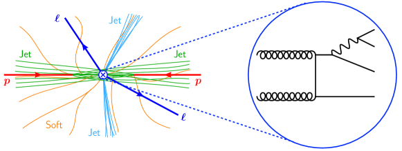
Figure 1: Schematic LHC collision. The collinear (green and blue) and soft radiation (orange) are described dynamically in SCET. The hard scattering (zoomed in on the right) is encoded in matching coefficients.

2 Helicity operators

We start by constructing quarks and gluon fields with definite helicity and then use this to construct our helicity operator basis. We will need the (conjugate) spinor with helicity $\pm$

$$|p\pm\rangle=\frac{1\pm\gamma_{5}}{2}\,u(p)\,,\qquad\langle p\pm|=\mathrm{sgn}(p^{0})\,\bar{u}(p)\,\frac{1\mp\gamma_{5}}{2}\,,$$ (3)

and the polarization vector for an (outgoing) gluon with momentum $p$ (with reference vector $k$)

$$\varepsilon_{+}^{\mu}(p,k)=\frac{\langle p\!+\!|\gamma^{\mu}|k+\rangle}{\sqrt{2}\langle k\!-\!|p+\rangle}\,,\quad\varepsilon_{-}^{\mu}(p,k)=-\frac{\langle p\!-\!|\gamma^{\mu}|k-\rangle}{\sqrt{2}\langle k\!+\!|p-\rangle}\,.$$ (4)

The smallest building blocks of operators are the quark and gluon fields $\chi_{n,\omega}$ and ${\mathcal{B}}_{n,\omega\perp}^{\mu}$, where $n=(1,\hat{n})$ denotes the collinear direction and $\omega=(1,-\hat{n})\cdot p$ is the large component of its momentum $p$. These fields are invariant under collinear gauge transformations through the inclusion of Wilson lines. We define a gluon field of definite helicity by

$${\mathcal{B}}^{a}_{i\pm}=-\varepsilon_{\mp\mu}(n_{i},\bar{n}_{i})\,{\mathcal{B}}^{a\mu}_{n_{i},\omega_{i}\perp_{i}}\,.$$ (5)

This definition is chosen such that that at tree level,

$$\bigl{\langle}g_{\lambda}^{a}(p)\bigr{|}{\mathcal{B}}_{i\lambda^{\prime}}^{a^{\prime}}\bigr{|}0\bigr{\rangle}=\delta_{\lambda,\lambda^{\prime}}\,\delta^{aa^{\prime}}\,\tilde{\delta}(\tilde{p}_{i}-p)\,,\qquad\bigl{\langle}0\bigr{|}{\mathcal{B}}_{i\lambda^{\prime}}^{a^{\prime}}\bigr{|}g_{\lambda}^{a}(p)\bigr{\rangle}=(1-\delta_{\lambda,\lambda^{\prime}})\,\delta^{aa^{\prime}}\,\tilde{\delta}(\tilde{p}_{i}+p)\,,$$ (6)

where the delta function $\tilde{\delta}$ only fixes the large momentum component $\tilde{p}_{i}=\omega_{i}n_{i}/2$. Exploiting that fermions come in pairs, we define fermion vectors currents of definite helicity

$$J_{ij+}^{{\bar{\alpha}}\beta}=\frac{\sqrt{2}\,\varepsilon_{-}^{\mu}(n_{i},n_{j})}{\sqrt{\phantom{2}\!\!\omega_{i}\,\omega_{j}}}\,\frac{\bar{\chi}^{\bar{\alpha}}_{i+}\,\gamma_{\mu}\chi^{\beta}_{j+}}{\langle n_{i}n_{j}\rangle}\,,\qquad J_{ij-}^{{\bar{\alpha}}\beta}=-\,\frac{\sqrt{2}\,\varepsilon_{+}^{\mu}(n_{i},n_{j})}{\sqrt{\phantom{2}\!\!\omega_{i}\,\omega_{j}}}\,\frac{\bar{\chi}^{\bar{\alpha}}_{i-}\,\gamma_{\mu}\chi^{\beta}_{j-}}{[n_{i}n_{j}]}\,,$$ (7)

which have similarly simple tree-level matrix elements.

It is now straightforward to write down the basis for a specific process. For example, for $ggq\bar{q}H$ the helicity basis consists of a total of six independent operators,

$$O_{++(\pm)}^{ab\,{\bar{\alpha}}\beta}=\frac{1}{2}\,{\mathcal{B}}_{1+}^{a}\,{\mathcal{B}}_{2+}^{b}\,J_{34\pm}^{{\bar{\alpha}}\beta}\,H_{5}\,,\quad O_{+-(\pm)}^{ab\,{\bar{\alpha}}\beta}={\mathcal{B}}_{1+}^{a}\,{\mathcal{B}}_{2-}^{b}\,J_{34\pm}^{{\bar{\alpha}}\beta}\,H_{5}\,,\quad O_{--(\pm)}^{ab\,{\bar{\alpha}}\beta}=\frac{1}{2}{\mathcal{B}}_{1-}^{a}\,{\mathcal{B}}_{2-}^{b}\,J_{34\pm}^{{\bar{\alpha}}\beta}\,H_{5}\,.$$ (8)

The symmetry factors in front of the operators account for identical fields. They ensure the validity of Eq. 11, leading to a simple matching equation.

For specific processes, it is convenient to decompose the color structure of the Wilson coefficients using a color basis $T_{k}^{a_{1}\cdots\alpha_{n}}$, where $k$ runs over the allowed color structures. This yields

$$C_{+\cdot\cdot(\cdot\cdot-)}^{a_{1}\cdots\alpha_{n}}=\sum_{k}C_{+\cdot\cdot(\cdot\cdot-)}^{k}T_{k}^{a_{1}\cdots\alpha_{n}}\equiv\bar{T}^{a_{1}\cdots\alpha_{n}}\vec{C}_{+\cdot\cdot(\cdot\cdot-)}\,.$$ (9)

For the $ggq\bar{q}H$ process a suitable color basis is given by

$$\bar{T}^{ab\alpha{\bar{\beta}}}=\Bigl{(}(T^{a}T^{b})_{\alpha{\bar{\beta}}}\,,\,(T^{b}T^{a})_{\alpha{\bar{\beta}}}\,,\,\textrm{tr}[T^{a}T^{b}]\,\delta_{\alpha{\bar{\beta}}}\Bigr{)}\,.$$ (10)

3 Matching

For our helicity operator basis, the tree-level matrix element of ${\mathcal{L}}_{\mathrm{hard}}$ is equal to the Wilson coefficient for the corresponding configuration of external particles,

$$\bigl{\langle}g_{1}g_{2}\cdots q_{n-1}\bar{q}_{n}\bigr{|}{\mathcal{L}}_{\mathrm{hard}}\bigr{|}0\bigr{\rangle}^{\mathrm{tree}}=C_{+\cdot\cdot(\cdot\cdot-)}^{a_{1}a_{2}\cdots\alpha_{n-1}{\bar{\alpha}}_{n}}(\tilde{p}_{1},\tilde{p}_{2},\ldots,\tilde{p}_{n-1},\tilde{p}_{n})\,,$$ (11)

where $g_{i}\equiv g_{\lambda_{i}}^{a_{i}}(p_{i})$ stands for a gluon with helicity $\lambda_{i}$, momentum $p_{i}$, color $a_{i}$, and analogously for (anti)quarks. This implies the tree-level matching equation

$$C_{+\cdot\cdot(\cdot\cdot-)}^{a_{1}\cdots{\bar{\alpha}}_{n}}(\tilde{p}_{1},\ldots,\tilde{p}_{n})=-\mathrm{i}{\mathcal{A}}^{\mathrm{tree}}(g_{1}\cdots\bar{q}_{n})\,,$$ (12)

where ${\mathcal{A}}^{\mathrm{tree}}$ is the tree-level QCD helicity amplitude.

In dimensional regularization, all loop corrections to the matrix element in Eq. 11 are scaleless and vanish. These corrections consist of UV poles, which get renormalized, and IR poles, which cancel in the matching because SCET is an effective theory of QCD. This implies,

$$C_{+\cdot\cdot(\cdot\cdot-)}^{a_{1}\cdots{\bar{\alpha}}_{n}}(\tilde{p}_{1},\ldots,\tilde{p}_{n})=-\mathrm{i}{\mathcal{A}}_{\mathrm{fin}}(g_{1}\cdots\bar{q}_{n})\equiv\frac{-\mathrm{i}\,\bar{T}^{a_{1}\cdots\bar{\alpha}_{n}}\widehat{Z}_{C}^{-1}\vec{\cal A}_{\rm ren}(g_{1}\cdots\bar{q}_{n})}{Z_{\xi}^{n_{q}/2}Z_{A}^{n_{g}/2}}\,.$$ (13)

Here $Z_{\xi}$, and $Z_{A}$ are the wave function renormalization of the quark and gluon field. $\widehat{Z}_{C}$ is the renormalization factor of the Wilson coefficient, which is a matrix in color space. At one-loop order ${\mathcal{A}}_{\mathrm{fin}}$ is simply the IR-finite part of the renormalized QCD helicity amplitude.

As an explicit example, we consider $ggq\bar{q}H$, for which the helicity operator basis was given in Eq. 8. The color decomposition of the QCD helicity amplitudes into partial amplitudes is

$${\mathcal{A}}\bigl{(}g_{1}g_{2}\,q_{3}{\bar{q}}_{4}H_{5}\bigr{)}=\mathrm{i}\!\!\sum_{\sigma\in S_{2}}\bigl{[}T^{a_{\sigma(1)}}T^{a_{\sigma(2)}}\bigr{]}_{\alpha_{3}{\bar{\alpha}}_{4}}A(\sigma(1),\sigma(2);3_{q},4_{\bar{q}};5_{H})\!+\mathrm{i}\,\textrm{tr}[T^{a_{1}}T^{a_{2}}]\,\delta_{\alpha_{3}{\bar{\alpha}}_{4}}B(1,2;3_{q},4_{\bar{q}};5_{H}).$$ (14)

Using the color basis in Eq. 10, we can read off the Wilson coefficients. E.g.

$$\vec{C}_{+-(+)}(\tilde{p}_{1},\tilde{p}_{2};\tilde{p}_{3},\tilde{p}_{4};\tilde{p}_{5})=\left(\!\!\!\begin{tabular}[]{c}$A_{\mathrm{fin}}(1^{+},2^{-};3_{q}^{+},4_{\bar{q}}^{-};5_{H})$\\ $A_{\mathrm{fin}}(2^{-},1^{+};3_{q}^{+},4_{\bar{q}}^{-};5_{H})$\\ $B_{\mathrm{fin}}(1^{+},2^{-};3_{q}^{+},4_{\bar{q}}^{-};5_{H})$\\ \end{tabular}\!\!\!\right)\,.$$ (15)

Charge conjugation invariance halves the number of independent Wilson coefficients.

4 Properties

Our operator basis is automatically crossing symmetric, because the gluon fields ${\mathcal{B}}_{i\pm}$ can absorb or emit a gluon, and the quark current $J_{ij\pm}$ can destroy or produce a quark-antiquark pair, or destroy and create a quark or antiquark.

The helicity operator basis has simple behavior under discrete symmetries. For example,

$$\mathrm{C}\,{\mathcal{B}}^{a}_{i\pm}\,T^{a}_{\alpha{\bar{\beta}}}\,\mathrm{C}=-{\mathcal{B}}^{a}_{i\pm}T^{a}_{\beta{\bar{\alpha}}}\,,\quad\mathrm{C}\,J^{{\bar{\alpha}}\beta}_{ij\pm}\,\mathrm{C}=-J^{{\bar{\beta}}\alpha}_{ji\mp}\,,$$ (16)

Charge conjugation and parity invariance reduce the number of independent Wilson coefficients.

Since the polarizations of gluons can be treated in $d$ rather than 4 dimensions, it is natural to ask whether our helicity operator basis is complete. Operators with $\epsilon$-dimensional polarizations do arise in the matching for states with physical polarizations. They are also not generated by the renormalization group evolution: The only communication between collinear sectors is through soft radiation, which does not carry spin and therefore cannot change helicity.

5 Conclusions and outlook

We have described a helicity operator basis, that makes it straightforward to write down the complete basis for a hard scattering process. It also facilitates the matching from fixed-order calculations onto SCET, since the matching coefficients are directly given in terms of the color-ordered helicity amplitudes. We demonstrated its ease by obtaining the Wilson coefficients for $pp\to H+0,1,2$ jets, $pp\to W/Z/\gamma+0,1,2$ jets, and $pp\to 2,3$ jets at (next-to-)leading order [3].

The spin of the operators does not play a crucial role at leading power, as the helicities are simply summed over in Eq. 2. This is not true for color, since soft gluons can exchange color. However, at subleading power also the spin structure is essential, since soft gluons can then also transfer spin. Our helicity approach was key in constructing a basis of subleading operators [4].

Spin information also needs to be kept track of when matching between different SCET theories. For example, to describe two nearby hard jets one matches through an intermediate SCET where the two nearby jets are not separately resolved [5]. To keep track of this spin information in the matching, helicity fields proved particularly useful [6].

References

References

[1]
Z. Bern, et al.
Phys. Rev. D, 88:014025, 2013.
R. K. Ellis, et al.
JHEP, 01:012, 2009.
S. Badger, et al
Phys. Rev. D, 89:034019, 2014.
V. Hirschi, et al.
JHEP, 05:044, 2011.
G. Cullen, et al.
Eur. Phys. J., C72:1889, 2012.
F. Cascioli, et al.
Phys. Rev. Lett., 108:111601, 2012.
[2]
C. W. Bauer, et al.
Phys. Rev. D, 63:014006, 2000.
C. W. Bauer, et al.
Phys. Rev. D, 63:114020, 2001.
C. W. Bauer and I. W. Stewart.
Phys. Lett. B, 516:134–142, 2001.
C. W. Bauer, et al.
Phys. Rev. D, 65:054022, 2002.
[3]
I. Moult, I. W. Stewart, F. J. Tackmann, and W. J. Waalewijn.
Phys. Rev. D, 93:094003, 2016.
[4]
Daniel W. Kolodrubetz, Ian Moult, and Iain W. Stewart.
arXiv:1601.02607.
[5]
C. W. Bauer, et al.
Phys. Rev. D, 85:074006, 2012.
[6]
Piotr Pietrulewicz, Frank J. Tackmann, and Wouter J. Waalewijn.
arXiv:1601.05088.