A globally convergent method for a 3-D inverse medium problem for the generalized Helmholtz equation

Abstract

A 3-D inverse medium problem in the frequency domain is considered. Another name for this problem is Coefficient Inverse Problem. The goal is to reconstruct spatially distributed dielectric constants from scattering data. Potential applications are in detection and identification of explosive-like targets. A single incident plane wave and multiple frequencies are used. A new numerical method is proposed. A theorem is proved, which claims that a small neigborhood of the exact solution of that problem is reached by this method without any advanced knowledge of that neighborhood. We call this property of that numerical method “global convergence”. Results of numerical experiments for the case of the backscattering data are presented.

Key Words: global convergence, coefficient inverse problem, frequency domain

2010 Mathematics Subject Classification: 35R30.

1 Introduction

Potential applications of the Inverse Medium Problem of this paper are in detection and identification of explosive-like targets using measurements of electromagnetic data. In the case of time dependent experimental data, this application was addressed in [2, 14, 19, 28, 29]. In the current paper, so as in [2, 14, 19, 28, 29], we calculate dielectric constants of targets for the case of the frequency dependent data. Of course, estimates of dielectric constants alone cannot differentiate between explosives and the clutter. On the other hand, the radar community is relying now only on the intensity of radar images [19]. Thus, we hope that the additional information about dielectric constants might lead in the future to the development of algorithms, which would better differentiate between explosives and the clutter.

An Inverse Medium Problem is the problem of determining one of coefficients of a PDE from boundary measurements. Another name for it is Coefficient Inverse Problem (CIP) or Inverse Scattering Problem. We are interested in a CIP for a generalized Helmholtz equation with the data resulting from a single measurement event. In other words, the boundary data are generated by a single direction of the incident plane wave and boundary measurements are conducted on an interval of frequencies. Thus, we use the minimal number of measurements for a CIP in the frequency domain. We call a numerical method for a CIP globally convergent if a theorem is proved, which claims that this method delivers at least one point in a sufficiently small neighborhood of the exact solution without any advanced knowledge of this neighborhood.

Currently there exist two types of globally convergent numerical methods for CIPs with single measurement data. The method of the first type was completely verified on electromagnetic experimental data, see, e.g. [2, 14, 19, 28, 29]. As to the method of the second type, it was initiated in [15] with a recently renewed interest [3, 16, 17]. In particular, in [16] numerical experiments are presented.

Methods of both types start from a CIP for a hyperbolic PDE. Next, the Laplace transform is applied with respect to time. It transforms the original hyperbolic PDE in the equation

$$\Delta w-s^{2}c\left(x\right)w=-\delta\left(x-x_{0}\right),x\in\mathbb{R}^{3},s>0$$ (1.1)

with the unknown coefficient $c\left(x\right)>0.$ Using the maximum principle, one can prove that $w>0$. Next, the function $\partial_{s}\left(\ln w/s^{2}\right)$ is considered and an integral differential PDE is obtained for this function. Integration is carried out from $s$ to $\infty.$ In the method of the first type, one truncates those integrals at a sufficiently large value $s:=\overline{s}.$ Next, one obtains a sequence of Dirichlet boundary value problems for elliptic PDEs. Solving those PDEs sequentially as well as updating residuals of those truncated integrals, one obtains points in a sufficiently small neighborhood of the exact solution without any advanced knowledge of that neighborhood. This corresponds to the above definition of the global convergence.

In the method of the second type, one does not truncate that integral. Rather, one uses Laugerre functions as well as Carleman Weight Function to construct a Tikhonov-like cost functional, which is strictly convex on any reasonable bounded set in a Sobolev space. This ensures the convergence of the gradient method to the unique minimum of that functional starting from any point of that bounded set. Convergence of minimizers to the exact solution when the level of the error in the data tends to zero is also guaranteed.

In this paper we develop a frequency domain analog of the globally convergent numerical method of the first type. The reason of this is that one can choose either of two types of measurements for the above application to detection and identification of explosives: either measurements of time dependent data, as in [2, 14, 28, 29], or measurements of frequency dependent data for a certain interval of frequencies.

One of the most difficult questions to address in this paper is that we need to work now with the complex valued analog of the function $w>0$ in (1.1). Let $\widetilde{w}$ be that analog. It is not immediately clear how to define $\mathop{\mathrm{I}m}\left(\log\widetilde{w}\right).$ To handle this difficulty, we modify our previous algorithm of [2, 14, 19, 28, 29], using the fact that $\partial\log\widetilde{w}=\partial\widetilde{w}/\widetilde{w}.$ So, we use only derivatives of $\log\widetilde{w}$. Moreover, the use of those derivatives leads us to a new scheme of the numerical method, as compared with the one of [2, 14, 19, 28, 29]. The second difficult question to address here, as compared with [2, 14, 28, 29], is that, unlike (1.1), the maximum principle does not work for the generalized Helmholtz equation.

Globally convergent numerical methods for CIPs for the case of the data resulting from multiple measurements were developed in [10, 11]. We also refer to the survey [1] for numerical methods for CIPs in the frequency domain with multiple frequencies and to, e.g. [21, 22, 23, 24, 25] for some other inverse scattering problems in the frequency domain.

In Section 2 we formulate forward and inverse problems which we consider. In Section 3 we consider the asymptotic behavior of the solution of the forward problem when the frequency tends to infinity. In Section 4 we use the Lippmann-Schwinger equation to establish some properties of the solution of the forward problem. In Section 5 we describe our numerical method. In Section 6 we establish existence and uniqueness theorem of a certain auxiliary boundary value problem. Section 7 is devoted to the convergence analysis. Numerical implementation of our method and numerical experiments are described in Section 8. We briefly summarize our results in Section 9.

2 The statement of the inverse scattering problem in the frequency domain

Let $B\left(R\right)=\left\{\left|x\right|<R\right\}\subset\mathbb{R}^{3}$ be the ball of the radius $R$ centered at $0$. Let $\Omega_{1}\Subset\Omega\Subset B\left(R\right)$ be two domains with boundaries $\partial\Omega$ and $\partial\Omega_{1}$ and let the domain $\Omega$ be convex. Both boundaries belong to the class $C^{2+\alpha}$ for some $\alpha\in(0,1).$ Here and below $C^{m+\alpha}$ are Hölder spaces of complex valued functions, where $m\geq 0$ is an integer. For any domain $Q\subseteq\mathbb{R}^{3}$ with the $C^{m+\alpha}$ boundary $\partial Q$ the norm in $C^{m+\alpha}\left(\overline{Q}\right)$ of a complex valued function $v$ is defined in the natural manner as $\left\|v\right\|_{C^{m+\alpha}\left(\overline{Q}\right)}=\left\|\mathop{\mathrm{R}e}v\right\|_{C^{m+\alpha}\left(\overline{Q}\right)}+\left\|\mathop{\mathrm{I}m}v\right\|_{C^{m+\alpha}\left(\overline{Q}\right)}.$ If a function $v\in C^{m+\alpha}\left(\mathbb{R}^{3}\right),$ then we denote $\left\|v\right\|_{m+\alpha}=\left\|v\right\|_{C^{m+\alpha}\left(\mathbb{R}^{3}\right)}.$ We denote norms in the spaces $C^{m+\alpha}\left(\overline{\Omega}\right)$ as $\left|v\right|_{m+\alpha},\forall v\in C^{m+\alpha}\left(\overline{\Omega}\right).$ If two functions $f,g\in C^{\alpha}\left(\overline{\Omega}\right),$ then obviously $\left|fg\right|_{\alpha}\leq\left|f\right|_{\alpha}\left|g\right|_{\alpha}.$ For any complex valued function $f\in C^{m+\alpha}\left(\overline{\Omega}\right),$ we define

$$\left|\nabla f\right|_{m+\alpha}=\mathop{\displaystyle\sum}\limits_{j=1}^{3}\left|f_{x_{j}}\right|_{m+\alpha}.$$

Assume that the spatially distributed dielectric constant $c(x),x\in\mathbb{R}^{3}$ satisfies the following conditions:

$$c(x)\in C^{15}(\mathbb{R}^{3}),\quad c(x)=1+\beta(x),$$ (2.1)

$$\beta(x)\geq 0,\text{ }\beta(x)=0\quad\text{for }\>x\in\mathbb{R}^{3}\setminus\Omega_{1}.$$ (2.2)

The $C^{15}-$smoothness of the function $c\left(x\right)$ was used in [18] for the proof of an analog of Lemma 3.1 (Section 3). We consider the following generalized Helmholtz equation

$$\Delta u+k^{2}c(x)u=0,\quad x\in\mathbb{R}^{3},$$ (2.3)

where $u\left(x,k\right)$ is the complex valued wave field and $k>0$ is the frequency. Let the incident plane wave $u_{0}\left(x,k\right)=\exp\left(-ikx_{3}\right)$ propagates along the positive direction of the $x_{3}-$axis. The total wave field

$$u\left(x,k\right)=u_{0}\left(x,k\right)+u_{\mathrm{sc}}\left(x,k\right),$$ (2.4)

is the solution of equation (2.3), which satisfies the radiation condition at the infinity,

$$\frac{\partial u_{\mathrm{sc}}}{\partial r}+iku_{\mathrm{sc}}=o(r^{-1}),\>\>r=|x|\rightarrow\infty.$$ (2.5)

Here $u_{\mathrm{sc}}(x,k)$ denotes the scattering wave. It is well known that the problem (2.3)-(2.5) has unique solution $u\left(x,k\right)\in C^{2+\alpha}\left(\mathbb{R}^{3}\right),$ see Theorems 8.3 and 8.7 in [6] as well as Section 4. Furthermore, Theorem 6.17 of [7] implies that the function $u\left(x,k\right)\in C^{16+\alpha}\left(\mathbb{R}^{3}\right).$ We consider the following inverse problem:

Problem 2.1 (Coefficient Inverse Problem (CIP)).

Let $\underline{k}$ and $\overline{k}$ be two constants such that $0<\underline{k}<\overline{k}.$ Assume that the function $g\left(x,k\right)$ is known, where

$$g\left(x,k\right)=u\left(x,k\right),\text{ \ }x\in\partial\Omega,k\in\left[\underline{k},\overline{k}\right].$$ (2.6)

Determine the function $\beta\left(x\right)$ for $x\in\Omega.$

Since $c(x)=1$ in $\mathbb{R}^{3}\setminus\Omega$, the function $u_{sc}(x,k)$ solves the following problem outside of the domain $\Omega$

$$\begin{array}[]{rcll}\Delta u_{\mathrm{sc}}+k^{2}u_{\mathrm{sc}}&=&0&\mbox{in }\mathbb{R}^{3}\setminus\overline{\Omega},\\ u_{\mathrm{sc}}&=&g-u_{0}&\mbox{on }\partial\Omega,\\ \partial_{r}u_{\mathrm{sc}}+iku_{\mathrm{sc}}&=&o(r^{-1})&\mbox{as }r\rightarrow\infty.\end{array}$$ (2.7)

The problem (2.7) has unique solution $u_{\mathrm{sc}}\in C^{2}\left(\mathbb{R}^{3}\setminus\overline{\Omega}\right)\cap C\left(\mathbb{R}^{3}\setminus\Omega\right)$, see Lemma 3.8 and Theorem 3.9 in [6]. Also, since we have established above that $u\left(x,k\right)\in C^{2+\alpha}\left(\mathbb{R}^{3}\right),$ then $u_{\mathrm{sc}}\in C^{2+\alpha}\left(\mathbb{R}^{3}\setminus\Omega\right).$ Hence, the knowledge of the function $u_{\mathrm{sc}}(x,k)$ outside of the domain $\Omega$ yields the additional boundary data $g_{1}\left(x,k\right),$ where

$$g_{1}(x,k)=\partial_{n}u(x,k),\quad x\in\partial\Omega,k\in[\underline{k},\overline{k}].$$ (2.8)

Even though we assume that the boundary measurements in (2.6) are conducted on the entire boundary $\partial\Omega,$ this is done for the analytical purpose only. In our computations we assume that we have only backscattering data, which better suits our above mentioned target application to imaging and identification of mine-like targets. We complement the backscattering data on the rest of the boundary $\partial\Omega$ by suitable values, see Section 8.

Since we use here only a single direction of the propagation of the incident plane wave $u_{0}\left(x,k\right),$ this is a problem with single measurement data. All currently known uniqueness theorems for $n-$dimensional CIPs, $n\geq 2,$ with single measurement data are proven using the method of [5]. This method is based on Carleman estimates. Many publications of different authors have discussed this method. Since the current work is not a survey of the technique of [5], we refer here only to a few such publications [2, 9, 12, 13, 31, 33]. In particular, [13] and [33] are surveys of that method. However, the technique of [5] works only if zero in the right hand side of (2.3) is replaced by such a function $f\in C\left(\overline{\Omega}\right),$ which does vanish in $\overline{\Omega}.$ Thus, since we study a numerical method here rather than the question of uniqueness, we assume uniqueness of our CIP.

We model the propagation of the electric wave field in $\mathbb{R}^{3}$ by the solution of the problem (2.3)-(2.5). This modeling was numerically justified in [4]. It was demonstrated numerically in [4] that this modeling can replace the modeling via the full Maxwell’s system, provided that only a single component of the electric field is incident upon the medium. Then this component dominates two others and its propagation is well governed by the time domain analog of equation (2.3). This conclusion was verified via accurate imaging using electromagnetic experimental data in, e.g. Chapter 5 of [2] and [14, 19, 28, 29].

3 The asymptotic behavior of the function $u\left(x,k\right)$ as $k$ tends to infinity

To establish this asymptotic behavior, we use geodesic lines generated by the function $c(x).$ Hence, we consider these lines in this section. The discussion of this section is a modification of the corresponding discussion of [18]. The Riemannian metric generated by the function $c(x)$ is

$$d\tau=\sqrt{c\left(x\right)}\left|dx\right|,|dx|=\sqrt{(dx_{1})^{2}+(dx_{2})^{2}+(dx_{3})^{2}}.$$

Consider the plane $P=\left\{x_{3}=-R\right\}.$ Then $P\cap\overline{\Omega}=\varnothing.$ Consider unit vectors $e_{1}=\left(1,0,0\right)$, $e_{2}=\left(0,1,0\right),e_{3}=\left(0,0,1\right).$ An arbitrary point $\xi_{0}\in P$ can be represented as

$$\xi_{0}=\xi_{0}(\eta_{1},\eta_{2})=\eta_{1}e_{1}+\eta_{2}e_{2}-Re_{3},\quad(\eta_{1},\eta_{2})\in\mathbb{R}^{2}.$$ (3.1)

Let the function $\tau(x)$ be the solution of the following Cauchy problem for the eikonal equation:

$$\left\{\begin{array}[]{c}\left(\nabla\tau(x)\right)^{2}=c(x),\\ \tau(x)=x_{3}\text{ for }x_{3}\leq-R.\end{array}\right.$$ (3.2)

It is well known that $|\tau(x)|$ is the Riemannian distance between the point $x$ and the plane $P$. Physically, $|\tau(x)|$ is the travel time between the point $x$ and the plane $P$. To find the function $\tau(x)$ for $x_{3}>-R,$ it is necessary to solve the problem (3.2). It is well known that to solve this problem, one needs to solve a system of ordinary differential equations. These equations also define geodesic lines of the Riemannian metric. They are (see, e.g. [26]):

$$\frac{d\xi}{ds}=\frac{p}{c(\xi)},\quad\frac{dp}{ds}=\frac{1}{2}\nabla\left(\ln c(\xi)\right),\quad\frac{d\tau}{ds}=1,$$ (3.3)

where $s$ is a parameter and $p=\nabla\tau(\xi)$. Consider an arbitrary point $\xi_{0}(\eta_{1},\eta_{2})\in P$ and the solution of the equations (3.3) with the Cauchy data

$$\xi|_{s=0}=\xi_{0}(\eta_{1},\eta_{2}),\quad p|_{s=0}=\sqrt{c(\xi_{0}(\eta_{1},\eta_{2}))}e_{3},\quad\tau|_{s=0}=0,$$ (3.4)

The solution of the problem (3.3), (3.4) defines the geodesic line which passes through the point $\xi_{0}(\eta_{1},\eta_{2})$ in the direction $e_{3}$. Hence, this line intersects the plane $P$ orthogonally. For $s>0$ this solution determines the geodesic line $\xi=r_{1}(s,\eta_{1},\eta_{2})$ and the vector $p=r_{2}(s,\eta_{1},\eta_{2}).$ This vector lays in the tangent direction to that geodesic line. It is well known from the theory of Ordinary Differential Equations that if the function $c(x)\in C^{m}(\mathbb{R}^{3})$, $m\geq 2$, then $r_{1}$ and $r_{2}$ are $C^{m-1}-$smooth functions.

By (3.1) and (3.4)

$$\frac{\partial\xi}{\partial\eta_{1}}\Big{|}_{s=0}=e_{1},\quad\frac{\partial\xi}{\partial\eta_{2}}\Big{|}_{s=0}=e_{2}.$$ (3.5)

Noting that $c(\xi_{0}(\eta_{1},\eta_{2}))=1,$ we obtain from (3.4)

$$\frac{d\xi}{ds}\Big{|}_{s=0}=\frac{\sqrt{c(\xi_{0}(\eta_{1},\eta_{2}))}}{c(\xi_{0}(\eta_{1},\eta_{2}))}e_{3}=e_{3}.$$

Hence,

$$\left|\frac{\partial(\xi_{1},\xi_{2},\xi_{3})}{\partial(s,\eta_{1},\eta_{2})}\right|_{s=0}=1\neq 0.$$ (3.6)

By (3.6) the equality $x=r_{1}(s,\eta_{1},\eta_{2})$ can be uniquely solved with respect to $s,\eta_{1},\eta_{2}$ for those points $x$ which are sufficiently close to the plane $P$, as $s=s(x),\eta_{1}=\eta_{1}(x),\eta_{2}=\eta_{2}(x).$ Hence, the equation

$$\xi=r_{1}(s,\eta_{1}(x),\eta_{2}(x))=\widehat{r}_{1}(s,x),\>s\in\left[0,s(x)\right]$$

defines the geodesic line $\Gamma(x)$ that passes through points $x$ and $\xi_{0}(\eta_{1}(x),\eta_{2}(x)):=\xi_{0}(x)$ and intersects the plane $P$ orthogonally. Extend the curve $\Gamma(x)$ for $x_{3}<-R$ as the straight line by the equation $\xi=\xi_{0}(x)+se_{3}$, $s<0$. The Riemannian distance between points $x$ and $\xi_{0}(x)$ is $s(x)=\tau(x)$. Note that $\widehat{r}_{j}(s,x)=r_{j}(s,\eta_{1}(x),\eta_{2}(x)),j=1,2$ are $C^{m-1}-$smooth functions of their arguments. Since $\widehat{r}_{2}(s,x)=\nabla_{x}\tau(x)$, then $\tau(x)$ is the $C^{m}-$smooth function. In our case $\tau(x)$ is $C^{15}-$smooth function of $x$ for those points $x$ which are sufficiently close to the plane $P$.

We have constructed above the family of geodesic lines $\Gamma(x)$ only “locally”, i.e. only for those points $x$ which are located sufficiently close to the plane $P.$ However, we need to consider these lines “globally”. Hence, everywhere below we rely on the following Assumption:

Assumption 3.1. We assume that above constructed geodesic lines satisfy the regularity condition in $\mathbb{R}^{3}$. In other words, for each point $x\in\mathbb{R}^{3}$ there exists a single geodesic line $\Gamma\left(x\right)$ connecting $x$ with the plane $P$ such that $\Gamma\left(x\right)$  intersects $P$ orthogonally and the function $\tau(x)\in C^{15}(\mathbb{R}^{3})$.

A sufficient condition for the regularity of geodesic lines was derived in [27],

$$\sum_{i,j=1}^{3}\frac{\partial^{2}\ln c(x)}{\partial x_{i}\partial x_{j}}\xi_{i}\xi_{j}\geq 0,\>\forall x,\xi\in\mathbb{R}^{3}.$$

Define the function $A(x)$ as

$$A(x)=\left\{\begin{array}[]{rl}\exp\left(-\frac{1}{2}\int\limits_{\Gamma(x)}c^{-1}(\xi)\Delta_{\xi}\tau(\xi)d\sigma\right),&x_{3}>-R,\\ 1,&x_{3}\leq-R.\end{array}\right.$$ (3.7)

The reason of the second line of (3.7) is the second line of (3.2) as well as the fact that $\Gamma(x)$ is the straight line for $x_{3}\leq-R.$ Lemma 3.1 was proved in [18], see Theorem 1 and the formula (4.25) in this reference. In the proof of Theorem 1 of [18], the $C^{15}-$smoothness of the function $c(x)$ was essentially used.

Lemma 3.1. Assume that conditions (2.1) and (2.2) are satisfied. Also, let Assumption 3.1 be in place. Then the following asymptotic behavior of the solution $u\left(x,k\right)$ of the problem (2.3)-(2.5) holds:

$$u\left(x,k\right)=A(x)e^{-ik\tau\left(x\right)}\left(1+O\left(1/k\right)\right),k\rightarrow\infty,x\in\Omega.$$ (3.8)

Here $\left|O\left(1/k\right)\right|\leq B_{1}/k,\forall x\in\overline{\Omega},$ where the constant $B_{1}=B_{1}\left(\Omega,c\right)>0$ depends only on listed parameters.

Hence, it follows from this lemma and (3.7) that there exists a number $k_{0}\left(\Omega,c\right)>0$ depending only on listed parameters such that

$$\left|O\left(1/k\right)\right|<1/2,\forall k\geq k_{0}\left(\Omega,c\right),\forall x\in\overline{\Omega}.$$ (3.9)

$$u\left(x,k\right)\neq 0,\forall x\in\overline{\Omega},\forall k\geq k_{0}\left(\Omega,c\right).$$ (3.10)

4 Using the Lippmann-Schwinger equation

In this section we use the Lippmann-Schwinger equation to derive some important facts, which we need both for our algorithm and for the convergence analysis. We are essentially using here results of Chapter 8 of the book of Colton and Kress [6]. In accordance with the regularization theory, we need to assume that there exists unique exact solution $c^{\ast}$ of our CIP for the noiseless data $g^{\ast}\left(x,k\right)$ in (2.6) [2, 30]. Everywhere below the superscript “$\ast$” denotes functions generated by $c^{\ast}.$

Denote

$$\Phi\left(x,y\right)=\frac{\exp\left(-i\overline{k}\left|x-y\right|\right)}{4\pi\left|x-y\right|},x\neq y.$$

In this section the function $\beta\in C^{\alpha}\left(\overline{\Omega}\right)$ and satisfies condition (2.2). The Lippmann-Schwinger equation for the function $u\left(x\right):=u\left(x,\overline{k}\right)$ is

$$u\left(x\right)=\exp\left(-i\overline{k}x_{3}\right)+\overline{k}^{2}\mathop{\displaystyle\int}\limits_{\Omega}\Phi\left(x,y\right)\beta(y)u\left(y\right)dy.$$ (4.1)

If the function $u\left(x\right)$ satisfies equation (4.1) for $x\in\Omega,$ then we can extend it for $x\in\mathbb{R}^{3}\diagdown\Omega$ via substitution these points $x$ in the right hand side of (4.1). Hence, to solve (4.1), it is sufficient to find the function $u\left(x\right)$ only for points $x\in\Omega.$ Consider the linear operator $K_{\beta}$ defined as

$$\left(K_{\beta}u\right)\left(x\right)=\overline{k}^{2}\mathop{\displaystyle\int}\limits_{{\Omega}}\Phi\left(x,y\right)\beta(y)u\left(y\right)dy.$$ (4.2)

It follows from Theorem 8.1 of [6] that

$$K_{\beta}:C^{\alpha}\left(\overline{\Omega}\right)\rightarrow C^{2+\alpha}\left(\mathbb{R}^{3}\right)\text{ and }\left\|K_{\beta}u\right\|_{2+\alpha}\leq B_{2}|\beta|_{\alpha}\left|u\right|_{\alpha}.$$ (4.3)

Here and below $B_{2}=B_{2}\left(\beta,\overline{k},\Omega_{1},\Omega\right)>0$ denotes different constants which depend only on listed parameters. Therefore, the operator $K_{\beta}$ maps $C^{\alpha}\left(\overline{\Omega}\right)$ in $C^{\alpha}\left(\overline{\Omega}\right)$ as a compact operator, $K_{\beta}:C^{\alpha}\left(\overline{\Omega}\right)\rightarrow C^{\alpha}\left(\overline{\Omega}\right)$. Hence, the Fredholm theory is applicable to equation (4.1). Lemmata 4.1 and 4.2 follow from Theorem 8.3 and Theorem 8.7 of [6] respectively.

Lemma 4.1. The function $u\in C^{2+\alpha}\left(\mathbb{R}^{3}\right)$ is a solution of the problem (2.3)-(2.5) if and only if it is a solution of equation (4.1).

Lemma 4.2. There exists unique solution $u\in C^{2+\alpha}\left(\mathbb{R}^{3}\right)$ of the problem (2.3)-(2.5). Consequently (Lemma 4.1) there exists unique solution $u\in C^{2+\alpha}\left(\mathbb{R}^{3}\right)$ of the problem (4.1) and these two solutions coincide. Furthermore, by the Fredholm theory $\left|u\right|_{\alpha}\leq B_{2}\left|\exp\left(-i\overline{k}x_{3}\right)\right|_{\alpha}.$ Also, with a different constant $B_{2}$, $\left|u\right|_{2+\alpha}\leq B_{2}\left|\exp\left(-i\overline{k}x_{3}\right)\right|_{2+\alpha}.$ 

Proof. We need to prove only the last estimate. By (4.3)

$$\left|K_{\beta}u\right|_{2+\alpha}\leq B_{2}|\beta|_{\alpha}\left|u\right|_{\alpha}\leq B_{2}\left|\exp\left(-i\overline{k}x_{3}\right)\right|_{\alpha}\leq B_{2}\left|\exp\left(-i\overline{k}x_{3}\right)\right|_{2+\alpha}.$$ (4.4)

On the other hand, by (4.1)

$$\left|u\right|_{2+\alpha}\leq\left|\exp\left(-i\overline{k}x_{3}\right)\right|_{2+\alpha}+\left|K_{\beta}u\right|_{2+\alpha}.$$ (4.5)

Thus, the desired estimate follows from (4.4) and (4.5).  $\square$

Lemma 4.3 follows from Lemmata 4.1, 4.2 and results of Chapter 9 of the book of Vainberg [32].

Lemma 4.3. For all $x\in\overline{\Omega},k>0$ the function $u\left(x,k\right)$ is infinitely many times differentiable with respect to $k$. Furthermore, $\partial_{k}^{n}u\in C^{2+\alpha}\left(\overline{\Omega}\right)$ and

$$\lim_{\omega\rightarrow 0,\omega\in\mathbb{R}}\left|\partial_{k}^{n}u\left(x,k+\omega\right)-\partial_{k}^{n}u\left(x,k\right)\right|_{2+\alpha}=0,\emph{\ }n=0,1,...\emph{\ }$$

Let the function $\chi\in C^{2}\left(\mathbb{R}^{3}\right)$ be such that

$$\chi\left(x\right)=\left\{\begin{array}[]{c}1,\text{ if }x\in\Omega_{1},\\ \text{between }0\text{ and }1,\text{ if }x\in\Omega\diagdown\Omega_{1},\\ 0,\text{ if }x\in\mathbb{R}^{3}\diagdown\Omega_{1}.\end{array}\right.$$ (4.6)

The existence of such functions is well known from the Real Analysis course. Consider a complex valued function $\rho\left(x\right)\in C^{\alpha}\left(\overline{\Omega}\right).$ Let $\widehat{\rho}\left(x\right)=\chi\left(x\right)\rho\left(x\right).$ Then

$$\widehat{\rho}\in C^{\alpha}\left(\mathbb{R}^{3}\right),\widehat{\rho}\left(x\right)=0\text{ in }\mathbb{R}^{3}\diagdown\Omega.$$ (4.7)

Theorem 4.1. Assume that the exact coefficient $c^{\ast}\left(x\right),$ satisfies conditions (2.1), (2.2). Let $\beta^{\ast}\left(x\right)=c^{\ast}\left(x\right)-1$. Let $u^{\ast}\left(x,\overline{k}\right)$ be the solution of the problem (2.3)-(2.5) in which $\beta\left(x\right)$ is replaced with $\beta^{\ast}\left(x\right).$ Consider equation (4.1), in which $\beta\left(x\right)$ is replaced with $\widehat{\rho}\left(x\right),$

$$u_{\rho}\left(x,\overline{k}\right)=\exp\left(-i\overline{k}x_{3}\right)+\overline{k}^{2}\mathop{\displaystyle\int}\limits_{\Omega}\Phi\left(x,y\right)\widehat{\rho}(y)u_{\rho}\left(y,\overline{k}\right)dy,x\in\Omega.$$ (4.8)

 Then there exists a sufficiently small number $\theta^{\ast}=\theta^{\ast}\left(\beta^{\ast},\overline{k},\chi,\Omega_{1},\Omega\right)\in\left(0,1\right)$ depending only on listed parameters such that if $\left|\rho-\beta^{\ast}\right|_{\alpha}\leq\theta$ and $\theta\in\left(0,\theta^{\ast}\right),$ then equation (4.8) has unique solution $u_{\rho}\in C^{\alpha}\left(\overline{\Omega}\right).$ Furthermore, the function $u_{\rho}\in C^{2+\alpha}\left(\mathbb{R}^{3}\right)$ and

$$\left|u_{\rho}\left(x,\overline{k}\right)-u^{\ast}\left(x,\overline{k}\right)\right|_{2+\alpha}\leq Z^{\ast}\theta,$$ (4.9)

 where the constant $Z^{\ast}=Z^{\ast}\left(\beta^{\ast},\overline{k},\chi,\Omega_{1},\Omega\right)>0$ depends only on listed parameters.

Proof. Below $Z^{\ast}$ denotes different positive constants depending on the above parameters. We have $\beta^{\ast}\left(x\right)=\chi\left(x\right)\beta^{\ast}\left(x\right)+\left(1-\chi\left(x\right)\right)\beta^{\ast}\left(x\right).$ Since by (2.2) the function $\beta^{\ast}\left(x\right)=0$ outside of the domain $\Omega_{1}$, then (4.6) implies that $\left(1-\chi\left(x\right)\right)\beta^{\ast}\left(x\right)\equiv 0.$ Hence, $\beta^{\ast}\left(x\right)=\chi\left(x\right)\beta^{\ast}\left(x\right).$ Hence, $\left(\widehat{\rho}-\beta^{\ast}\right)\left(x\right)=\chi\left(x\right)\left(\rho-\beta^{\ast}\right)\left(x\right).$ Hence, using notation (4.2), we rewrite equation (4.8) in the following equivalent form:

$$\left(I-K_{\beta^{\ast}}\right)u_{\rho}=\exp\left(-i\overline{k}x_{3}\right)+A_{\rho-\beta^{\ast}}\left(u_{\rho}\right),x\in\Omega,$$ (4.10)

$$A_{\rho-\beta^{\ast}}\left(u_{\rho}\right)\left(x\right)=\overline{k}^{2}\mathop{\displaystyle\int}\limits_{\Omega}\Phi\left(x,y\right)\chi\left(y\right)\left(\rho-\beta^{\ast}\right)(y)u_{\rho}\left(y,\overline{k}\right)dy,x\in\Omega.$$ (4.11)

The linear operator $A_{\rho-\beta^{\ast}}:C^{\alpha}\left(\overline{\Omega}\right)\rightarrow C^{\alpha}\left(\overline{\Omega}\right).$ We have for any function $p\in C^{\alpha}\left(\overline{\Omega}\right)$

$$\left|A_{\rho-\beta^{\ast}}\left(p\right)\right|_{\alpha}=\left|\overline{k}^{2}\mathop{\displaystyle\int}\limits_{\Omega}\Phi\left(x,y\right)\chi\left(y\right)\left(\rho-\beta^{\ast}\right)(y)p\left(y\right)dy\right|_{2+\alpha}\leq Z^{\ast}\theta|p|_{\alpha}.$$ (4.12)

Therefore,

$$\left\|A_{\rho-\beta^{\ast}}\right\|\leq Z^{\ast}\theta.$$ (4.13)

It follows from Lemma 4.2 and the Fredholm theory that the operator $\left(I-K_{\beta^{\ast}}\right)$ has a bounded inverse operator $T=\left(I-K_{\beta^{\ast}}\right)^{-1},T:C^{\alpha}\left(\overline{\Omega}\right)\rightarrow C^{\alpha}\left(\overline{\Omega}\right)$ and also

$$\left\|T\right\|\leq Z^{\ast}.$$ (4.14)

Hence, using (4.10), we obtain

$$u_{\rho}=T\left(\exp\left(-i\overline{k}x_{3}\right)\right)+\left(TA_{\rho-\beta^{\ast}}\right)\left(u_{\rho}\right).$$ (4.15)

It follows from (4.13) and (4.14) that there exists a sufficiently small number $\theta^{\ast}\in(0,1)$ depending on $\beta^{\ast}$, $\overline{k},$ $\chi,\Omega_{1},\Omega$ such that if $\theta\in\left(0,\theta^{\ast}\right)$ and $|\rho-\beta^{\ast}|_{\alpha}\leq\theta,$ then the operator $\left(TA_{\rho-\beta^{\ast}}\right):C^{\alpha}\left(\overline{\Omega}\right)\rightarrow C^{\alpha}\left(\overline{\Omega}\right)$ is contraction mapping. This implies uniqueness and existence of the solution $u_{\rho}\in C^{\alpha}\left(\overline{\Omega}\right)$ of equation (4.15), which is equivalent to equation (4.8). Also,

$$\left|u_{\rho}\right|_{\alpha}\leq Z^{\ast}\left|\exp\left(-i\overline{k}x_{3}\right)\right|_{\alpha},$$ (4.16)

with a different constant $Z^{\ast}.$ Furthermore, by (4.3) the function $u_{\rho}\in C^{2+\alpha}\left(\overline{\Omega}\right).$

We now prove estimate (4.9). Let $\widetilde{u}\left(x\right)=u^{\ast}\left(x,\overline{k}\right)-u_{\rho}\left(x,\overline{k}\right).$ Since $\left(I-K_{\beta^{\ast}}\right)u^{\ast}=\exp\left(-i\overline{k}x_{3}\right),$ we obtain the following analog of (4.10)

$$\left(I-K_{\beta^{\ast}}\right)\widetilde{u}=A_{\rho-\beta^{\ast}}\left(u_{{}_{\rho}}\right),x\in\Omega.$$ (4.17)

Hence, $\widetilde{u}=\left(TA_{\rho-\beta^{\ast}}\right)\left(u_{\rho}\right).$ Hence, (4.13) and (4.16) lead to

$$\left|\widetilde{u}\right|_{\alpha}\leq Z^{\ast}\theta.$$ (4.18)

Next, we rewrite (4.17) as

$$\widetilde{u}=K_{\beta^{\ast}}\widetilde{u}+A_{\rho-\beta^{\ast}}\left(u_{\rho}\right),\text{ }x\in\Omega.$$ (4.19)

By (4.3) and (4.11) the right hand side of equation (4.19) belongs to the space $C^{2+\alpha}\left(\overline{\Omega}\right).$ Hence, using (4.3), (4.12), (4.16) and (4.18), we obtain from (4.19) that $\left|\widetilde{u}\right|_{2+\alpha}\leq Z^{\ast}\theta.$ $\square$

5 Numerical method

5.1 Some auxiliary functions

Starting from this subsection and until section 8 $x\in\Omega,$ and we do not consider $x\in\mathbb{R}^{3}\diagdown\Omega.$ We define in this subsection the logarithm of the complex valued function $u(x,k)$, $x\in\Omega,k>0$. We note that, except of subsection 5.3, we use only derivatives of $\log u$ and do not use $\log u$ itself. Since $\partial\log u=\partial u/u,$ then this eliminates the uncertainty linked with $\mathop{\mathrm{I}m}\left(\log u\right).$ Below $\overline{k}>\underline{k}>k_{0}\left(\Omega,c\right)$ and we consider $k\in\left[\underline{k},\overline{k}\right].$ The number $k_{0}\left(\Omega,c\right)$ was defined in (3.9), (3.10). Hence, by (3.10) $u\left(x,k\right)\neq 0$ for $k\in\left[\underline{k},\overline{k}\right],x\in\overline{\Omega}.$ It is convenient to consider in this section only $C^{2+\alpha}-$smoothness of the function $u\left(x,k\right),$ i.e. $u\in C^{2+\alpha}\left(\overline{\Omega}\right)$.

By a simple calculation, $\mathrm{curl}\left(\nabla u(x,\overline{k})/u(x,\overline{k})\right)=0$ in $\mathbb{R}^{3}$. Since $\Omega$ is a convex domain, then there exists a function $V\left(x\right)$, such that

$$\nabla V\left(x\right)=\frac{\nabla u\left(x,\overline{k}\right)}{u\left(x,\overline{k}\right)},x\in\overline{\Omega}.$$ (5.1)

By (5.1)

$$e^{-V(x)}\left(u(x,\overline{k})\nabla V(x)-\nabla u(x,\overline{k})\right)=0,x\in\overline{\Omega},$$

which implies $\nabla(e^{-V(x)}u(x,\overline{k}))=0$. Thus, there exists a constant $C$ such that $u(x,\overline{k})=Ce^{V(x)},x\in\overline{\Omega}.$ Since the function $V(x)$ is uniquely determined up to an addition of a constant, we can choose $V(x)$ such that $C=1$. In summary, we can find a function $V$ such that

$$u(x,\overline{k})=e^{V(x)},\mbox{or }V(x)=\log(u(x,\overline{k})).$$ (5.2)

Since the function $u\in C^{2+\alpha}\left(\overline{\Omega}\right),$ then it follows from (5.1) that $\nabla V\in C^{1+\alpha}\left(\overline{\Omega}\right)$.

By Lemma 4.3 the derivative $\partial_{k}u\left(x,k\right)\in C^{2+\alpha}\left(\overline{\Omega}\right)$ exists and the continuity property (LABEL:10) is valid. Hence, we can define the function $v(x,k)$ for all $k\in\left[\underline{k},\overline{k}\right],x\in\overline{\Omega}$ as

$$v(x,k)=-\int_{k}^{\overline{k}}\frac{\partial_{k}u(x,\kappa)}{u(x,\kappa)}d\kappa+V(x),x\in\overline{\Omega}.$$ (5.3)

Differentiate (5.3) with respect to $k$. We obtain $\partial_{k}v(x,k)=\partial_{k}u(x,k)/u(x,k)$. Therefore,

$$e^{-v(x,k)}\left(u(x,k)\partial_{k}v(x,k)-\partial_{k}u(x,k)\right)=0,x\in\overline{\Omega},$$

which implies $\partial_{k}(e^{-v(x,k)}u(x,k))=0$ or $u(x,k)=C(x)e^{v(x,k)}$ for all $k\in\left[k_{0}\left(\Omega,c\right),\overline{k}\right],x\in\overline{\Omega}.$ In particular, taking $k=\overline{k}$ and using (5.2), we obtain $C\left(x\right)=1.$

Lemma 5.1.

For each $k\in\left[\underline{k},\overline{k}\right]$ the gradient $\nabla v\in C^{1+\alpha}\left(\overline{\Omega}\right).$ In addition for all $x\in\overline{\Omega}:$

1. $u(x,k)=e^{v(x,k)}$,

2. $\nabla v(x,k)=\nabla u(x,k)/u(x,k),$

3. $\partial_{k}v(x,k)=\displaystyle\frac{\partial_{k}u(x,k)}{u(x,k)}$,

4. $$\Delta v(x,k)+(\nabla v(x,k))^{2}=-k^{2}c(x).$$ (5.4)

Proof. The smoothness of $\nabla v$ follows from $\nabla V\in C^{1+\alpha}\left(\overline{\Omega}\right)$ and from (5.3). Item 1 was established above. The differentiation of the equality of item 1 leads to item 2. Item 3 follows from (5.3). Equation (5.4) follows from item 1 and (2.3). $\square$

Thus, $V\left(x\right)$ is our tail function. The exact tail function, which is generated by the exact coefficient $c^{\ast}\left(x\right),$ is $V^{\ast}\left(x\right)=\log u^{\ast}\left(x,\overline{k}\right).$

5.2 Integral differential equation

Consider the function $q\left(x,k\right)$ defined as

$$q(x,k)=\partial_{k}v(x,k)=\frac{\partial_{k}u(x,k)}{u(x,k)},\quad x\in\Omega,k\in\left(\underline{k},\overline{k}\right).$$ (5.5)

Here, we have used item 3 in Lemma 5.1 for the latter fact. By (5.3)

$$v(x,k)=-\int_{k}^{\overline{k}}q(x,\kappa)d\kappa+V(x),\quad x\in\Omega,k\in(\underline{k},\overline{k}).$$ (5.6)

Note that $V\left(x\right)=v\left(x,\overline{k}\right).$ We call $V\left(x\right)$ the “tail function”. We note that the number $\overline{k}$ plays the role of the regularization parameter of our numerical method. A convergence analysis of our method for $\overline{k}\rightarrow\infty$ is a very challenging problem and we do not yet know how to address it. The differentiation of (5.4) with respect to $k$ leads to

$$\Delta q(x,k)+2\nabla q(x,k)\nabla v(x,k)=-2kc(x)=2(\Delta v+(\nabla v)^{2})/k.$$

This,  and (5.6) imply that for all $k\in\left[\underline{k},\overline{k}\right]$

$$k\Delta q(x,k)+2k\nabla q(x,k)\nabla\left(-\int_{k}^{\overline{k}}q(x,\kappa)d\kappa+V(x)\right)$$ (5.7)

$$= 2\left(\Delta\left(-\int_{k}^{\overline{k}}q(x,\kappa)d\kappa+V(x)\right)+\left(\nabla\left(-\int_{k}^{\overline{k}}q(x,\kappa)d\kappa+V(x)\right)\right)^{2}\right).$$

By Lemma 5.1 as well as by (2.6) and (5.5), the function $q$ satisfies the Dirichlet boundary condition

$$q(x,k)=\frac{\partial_{k}g(x,k)}{g(x,k)}=:\psi(x,k)\quad\mbox{on }\partial\Omega,\psi\left(x,k\right)\in C^{2+\alpha}\left(\partial\Omega\right),\forall k\in\left[\underline{k},\overline{k}\right].$$ (5.8)

We have obtained a nonlinear integral differential equation (5.7) for the function $q\left(x,k\right)$ with the Dirichlet boundary condition (5.8). Both functions $q$ and $V$ in (5.7) are unknown. To solve our inverse problem, both these functions need to be approximated. Here is a brief description how do we do this. We start from finding a first approximation $V_{0}\left(x\right)$ for the tail function, see subsection 5.3. To approximate the function $q$, we iteratively solve the problem (5.7), (5.8) inside of the domain $\Omega.$ Given an approximation for $q$, we find the next approximation for the unknown coefficient $c,$ and then we solve the Lippman-Schwinger equation inside of the domain $\Omega$ with this updated coefficient $c$. Next, we find the new approximation for the gradient of the tail function $V$ via (5.1) as $\nabla V=\nabla u\left(x,\overline{k}\right)/u\left(x,\overline{k}\right)$ and similarly for the new approximation for $\Delta V=\mathop{\mathrm{d}iv}\left(\nabla V\right)$. So, this is an analog of the well known predictor-corrector procedure, where updates for $V$ are predictors and updates for $q$ and $c$ are correctors.

5.3 The first approximation $V_{0}\left(x\right)$ for the tail function

Consider the exact coefficient $c^{\ast}\left(x\right)$ and assume that conditions (2.1), (2.2) as well as Assumption 3.1 hold for $c^{\ast}\left(x\right)$. Then (3.8) holds for $c\left(x\right):=c^{\ast}\left(x\right).$ Assume that the number $\overline{k}$ is sufficiently large. For all $k\geq\overline{k}$ drop the term $O\left(1/k\right)$ in (3.8). Hence, we approximate the function $u^{\ast}\left(x,k\right)$ as

$$u^{\ast}\left(x,k\right)=A^{\ast}\left(x\right)e^{-ik\tau^{\ast}\left(x\right)},k\geq\overline{k}.$$ (5.9)

We set

$$\log u^{\ast}\left(x,k\right)=\ln A^{\ast}\left(x\right)-ik\tau^{\ast}\left(x\right)\text{ for }k\geq\overline{k}.$$

Hence,

$$\log u^{\ast}\left(x,k\right)=-ik\tau^{\ast}\left(x\right)\left(1+O\left(\frac{1}{k}\right)\right),k\rightarrow\infty.$$ (5.10)

Drop again the term $O\left(1/k\right)$ in (5.10). Next, set $k=\overline{k}.$ Hence, we approximate the exact tail function $V^{\ast}\left(x\right)$ for $k=\overline{k}$ as

$$V^{\ast}\left(x\right)=-i\overline{k}\tau^{\ast}\left(x\right).$$ (5.11)

Using (5.5) and (5.9), we obtain

$$q^{\ast}\left(x,\overline{k}\right)=-i\tau^{\ast}\left(x\right).$$ (5.12)

Set in equation (5.7) $k:=\overline{k},q\left(x,\overline{k}\right):=q^{\ast}\left(x,\overline{k}\right),V(x):=V^{\ast}(x).$ Next, substitute in the resulting equation formulae (5.11) and (5.12). Also, use (5.8) for $\psi:=\psi^{\ast}$. We obtain

$$\begin{array}[]{c}\Delta\tau^{\ast}=0\text{ in }\Omega,\\ \tau^{\ast}\mid_{\partial\Omega}=i\psi^{\ast}\left(x,\overline{k}\right).\end{array}$$ (5.13)

Thus, we have obtained the Dirichlet boundary value problem (5.13) for the Laplace equation with respect to the function $\tau^{\ast}\left(x\right)$. Recalling that $\partial\Omega\in C^{2+\alpha}$ and that the function $\psi^{\ast}\left(x,\overline{k}\right)\in C^{2+\alpha}\left(\partial\Omega\right)$ and applying the Schauder theorem [20], we obtain that there exists unique solution $\tau^{\ast}\in C^{2+\alpha}\left(\overline{\Omega}\right)$ of the problem (5.13).

In practice, however, we have the non-exact boundary data $\psi\left(x,k\right)$ rather than the exact data $\psi^{\ast}\left(x,k\right).$ Thus, we set the first approximation $V_{0}\left(x\right)$ for the tail function $V\left(x\right)$ as

$$V_{0}\left(x\right)=-i\overline{k}\tau\left(x\right),$$ (5.14)

where the function $\tau\left(x\right)$ is the $C^{2+\alpha}\left(\overline{\Omega}\right)-$solution of the following analog of is the solution of the problem (5.13):

$$\begin{array}[]{c}\Delta\tau=0\text{ in }\Omega,\\ \tau\mid_{\partial\Omega}=i\psi\left(x,\overline{k}\right).\end{array}$$ (5.15)

Theorem 5.1 estimates the difference between functions $V_{0}\left(x\right)$ and $V^{\ast}\left(x\right).$

Theorem 5.1. Assume that relations (5.11), (5.12), (5.14) and (5.15) are valid. Then there exists a constant $C=C\left(\Omega\right)>0$ depending only on the domain $\Omega$ such that

$$\left|V_{0}-V^{\ast}\right|_{2+\alpha}\leq C\overline{k}\left\|\psi\left(x,\overline{k}\right)-\psi^{\ast}\left(x,\overline{k}\right)\right\|_{C^{2+\alpha}\left(\partial\Omega\right)}.$$ (5.16)

Proof. Note that (5.13) follows from (5.7), (5.8), (5.11) and (5.12). Denote $\widetilde{\tau}\left(x\right)=\tau\left(x\right)-\tau^{\ast}\left(x\right).$ Then (5.13) and (5.15) imply that

$$\begin{array}[]{c}\Delta\widetilde{\tau}=0,x\in\Omega,\\ \widetilde{\tau}\mid_{\partial\Omega}=i\left(\psi-\psi^{\ast}\right)\left(x,\overline{k}\right).\end{array}$$

Hence, the Schauder theorem [20] leads to (5.16). $\square$

Remarks 5.1:

1. Theorem 5.1 means that the accuracy of the approximation of the exact tail function $V^{\ast}$ by the function $V_{0}$ depends only on the accuracy of the approximation of the exact boundary condition $\psi^{\ast}\left(x,\overline{k}\right)$ by the boundary condition $\psi\left(x,\overline{k}\right).$ Let $\delta>0$ be the level of the error in the boundary data at $k:=\overline{k}$, i.e. $\left\|\psi\left(x,\overline{k}\right)-\psi^{\ast}\left(x,\overline{k}\right)\right\|_{C^{2+\alpha}\left(\partial\Omega\right)}\leq\delta.$ Hence, if $\delta$ is sufficiently small, then, by (5.16), the norm $\left|V_{0}-V^{\ast}\right|_{2+\alpha}$ is also sufficiently small. In the regularization theory the error in the data $\delta$ is always assumed to be sufficiently small [2, 30]. Thus, we have obtained the tail function $V_{0}$ in a sufficiently small neighborhood of the exact tail function $V^{\ast}$. Furthermore, in doing so, we have not used any a priori knowledge about a sufficiently small neighborhood of the function $V^{\ast}.$ The smallness of that neighborhood depends only on the level of the error in the boundary data. The latter is exactly what is required in the regularization theory.

2. Thus, the global convergence property is achieved just at the start of our iterative process. It is achieved due to two factors. The first factor is the elimination of the unknown coefficient from equation (5.4) and obtaining the integral differential equation (5.7). The second factor is dropping the term $O\left(1/k\right)$ in (5.9) and (5.10).

3. Still, our numerical experience shows that we need to do more iterations to obtain better accuracy. These iterations are described in subsection 5.4.

4. We point out that we use the approximations (5.9), (5.11) and (5.12) of the exact tail function $V^{\ast}\left(x\right)$ only on the first iteration of our method: to obtain the first approximation $V_{0}\left(x\right)$ for the tail function. However, we do not use them on follow up iterations. On a deeper sense, these approximations are introduced because the problem of constructing globally convergent numerical methods for CIPs is well known to be a tremendously challenging one. Indeed, CIPs are both nonlinear and ill-posed. Thus, it makes sense to use such an approximation. Because of this approximation, one can also call our technique an approximately globally convergent numerical method, see section 1.1.2 in [2] as well as [19] for detailed discussions of the notion of the approximate global convergence.

5.4 The algorithm

Let $h>0$ be the partition step size of a uniform partition of the frequency interval $\left[\underline{k},\overline{k}\right]$,

$$\underline{k}=k_{N}<k_{N-1}<...<k_{1}<k_{0}=\overline{k},k_{j-1}-k_{j}=h.$$ (5.17)

Approximate the function $q\left(x,k\right)$ as a piecewise constant function with respect to $k\in\left[\underline{k},\overline{k}\right].$ Then (5.8) implies that the boundary condition $\psi\left(x,k\right),x\in\partial\Omega$ should also be approximated by a piecewise constant function with respect to $k\in\left[\underline{k},\overline{k}\right].$ Let

$$q\left(x,k\right)=q_{n}\left(x\right),\psi\left(x,k\right)=\psi_{n}\left(x\right),k\in\left[k_{n},k_{n-1}\right),n=1,...,N.$$ (5.18)

We set $q_{0}\left(x\right)\equiv 0.$ Denote

$$\overline{q_{n-1}}=\mathop{\displaystyle\sum}\limits_{j=0}^{n-1}q_{j}\left(x\right).$$ (5.19)

Hence, (5.6) becomes

$$v\left(x,k\right)=-\left(k_{n-1}-k\right)q_{n}\left(x\right)-h\overline{q_{n-1}}+V\left(x\right),k\in\left[k_{n},k_{n-1}\right).$$ (5.20)

Hence, the problem (5.7), (5.8) can be rewritten for $k\in\left[k_{n},k_{n-1}\right)$ as

$$\begin{array}[]{c}\left(2k_{n-1}-k\right)\Delta q_{n}-2k_{n-1}\left(k_{n-1}-k\right)\left(\nabla q_{n}\right)^{2}-2kh\nabla\overline{q_{n-1}}\nabla q_{n}\\ -4h\left(k_{n-1}-k\right)\nabla\overline{q_{n-1}}\nabla q_{n}-2\left(h\nabla\overline{q_{n-1}}\right)^{2}+2h\Delta\overline{q_{n-1}}\\ +2k\nabla q_{n}\nabla V+4\left(k_{n-1}-k\right)\nabla V\nabla q_{n}+4\nabla Vh\nabla\overline{q_{n-1}}=2\left(\Delta V+\left(\nabla V\right)^{2}\right),\\ q_{n}\mid_{\partial\Omega}=\psi_{n}\left(x\right).\end{array}$$ (5.21)

Assuming that the number $h$ is sufficiently small and that $h\overline{k}<<1,$ we now ignore those terms in (5.21), whose absolute values are $O\left(h\right)$ as $h\rightarrow 0$. We also assume in the convergence analysis that the number $\overline{k}-\underline{k}$ is sufficiently small. Hence, the number $\left|h\nabla\overline{q_{n-1}}\right|\leq\left(\overline{k}-\underline{k}\right)\max_{j}\sup_{x\in\Omega}\left|\nabla q_{j}\left(x\right)\right|$ is also small. However, we do not ignore $\left|h\nabla\overline{q_{n-1}}\right|.$ Still, we ignore in (5.21) the term $2\left(h\nabla\overline{q_{n-1}}\right)^{2}.$ Hence, we obtain from (5.21) for

$$\begin{array}[]{c}k_{n-1}\Delta q_{n}-2k\nabla q_{n}h\nabla\overline{q_{n-1}}+2k\nabla q_{n}\nabla V+2h\Delta\overline{q_{n-1}}\\ =2\left(\Delta V+\left(\nabla V\right)^{2}\right)-4\nabla Vh\nabla\overline{q_{n-1}},\text{ }x\in\Omega,k\in\left[k_{n},k_{n-1}\right),\\ q_{n}\mid_{\partial\Omega}=\psi_{n}\left(x\right).\end{array}$$ (5.22)

Even though the left hand side of equation (5.22) depends on $k$, it changes very little with respect to $k\in\left[k_{n},k_{n-1}\right)$ since the interval $\left[k_{n},k_{n-1}\right)$ is small. Still, to eliminate this $k-$dependence, we integrate both sides of equation (5.22) with respect to $k\in\left(k_{n},k_{n-1}\right)$ and then divide both sides of the resulting equation by $h$. We obtain

$$\begin{array}[]{c}\Delta q_{n}-A_{n}h\overline{\nabla q_{n-1}}\nabla q_{n}=\\ -A_{n}\nabla q_{n-1}\nabla V_{n-1}+2\left(\Delta V_{n-1}+\left(\nabla V_{n-1}\right)^{2}\right)/k_{n-1}\\ -4\nabla V_{n-1}h\nabla\overline{q_{n-1}}/k_{n-1}-2h\Delta\overline{q_{n-1}}/k_{n-1},\text{ }x\in\Omega,\\ q_{n}\mid_{\partial\Omega}=\psi_{n}\left(x\right),\end{array}$$ (5.23)

where $A_{n}=\left(1+k_{n}/k_{n-1}\right).$ Hence,

$$0<A_{n}<2.$$ (5.24)

We have replaced in (5.23) $V$ with $V_{n-1}$ since we will update tail functions in our iterative algorithm. In (5.23) the term $-A_{n}\nabla q_{n-1}\nabla V_{n-1}$ should actually be $-A_{n}\nabla q_{n}\nabla V_{n-1}.$ We have made this replacement for our convergence analysis. Indeed, for the exact solution $\nabla q_{n}^{\ast}=\nabla q_{n-1}^{\ast}+\left(\nabla q_{n}^{\ast}-\nabla q_{n-1}^{\ast}\right).$ By Lemma 4.3 $\left|\nabla q_{n}^{\ast}-\nabla q_{n-1}^{\ast}\right|=O\left(h\right),h\rightarrow 0$. The latter, the above dropped terms, whose absolute values are $O\left(h\right)$ as $h\rightarrow 0,$ as well as the approximations (5.18) are taken into account by the function $G_{n}^{\ast}\left(x\right)$ in (7.8) and (7.9) in our convergence analysis.

Algorithm 5.1 (Globally convergent algorithm).

2. Set $q_{0}\equiv 0,q_{1,0}=0,\nabla V_{1,0}=\nabla V_{0},$ where the vector $\nabla V_{0}$ is found as in Subsection 5.3.

3. For $n=1$ to $N$,

   2. Assume that $q_{n-1}$ and $\nabla V_{n-1}$ are found. Set $q_{n,0}=q_{n-1}$ and $\nabla V_{n,0}=\nabla V_{n-1}$.

   3. For $i=1$ to $m$ (for an integer $m\geq 1$)

      2. Assume that $q_{n,i-1}$ and $V_{n,i-1}$ are found. Find $q_{n,i}\in C^{2+\alpha}\left(\overline{\Omega}\right)$ as the solution of the Dirichlet boundary value problem:

         $$\begin{array}[]{c}\Delta q_{n,i}-A_{n}h\overline{\nabla q_{n-1}}\nabla q_{n,i}=\\ -A_{n}\nabla q_{n-1}\nabla V_{n,i-1}+2\left(\Delta V_{n,i-1}+\left(\nabla V_{n,i-1}\right)^{2}\right)/k_{n-1}\\ -4\nabla V_{n,i-1}h\overline{\nabla q_{n-1}}/k_{n-1}-2h\Delta\overline{q_{n-1}}/k_{n-1},\text{ }x\in\Omega,\\ q_{n,i}\mid_{\partial\Omega}=\psi_{n}\left(x\right).\end{array}$$ (5.25)

      3. Consider the vector function $\nabla v_{n,i}$,

         $$\nabla v_{n,i}\left(x\right)=-\left(hq_{n,i}\left(x\right)+h\overline{q_{n-1}}\left(x\right)\right)+\nabla V_{n,i-1}\left(x\right),\text{ }x\in\Omega.$$ (5.26)

         Using $\Delta v_{n,i}=\mathop{\mathrm{d}iv}\left(\nabla v_{n,i}\right),$ calculate the approximation $c_{n,i}\left(x\right)\in C^{\alpha}\left(\overline{\Omega}\right)$ for the target coefficient $c\left(x\right)$ as

         $$\beta_{n,i}(x) = -\frac{1}{k_{n}^{2}}(\Delta v_{n,i}(x)+(\nabla v_{n,i}(x))^{2})-1,$$ (5.27)

         $$c_{n,i}\left(x\right) = \beta_{n,i}(x)+1.$$ (5.28)

      4. Next, solve the Lippman-Schwinger equation (4.8), where $\widehat{\rho}(y)$ is replaced with $\chi\left(y\right)(c_{n,i}-1)\left(y\right).$ We obtain the function $u_{n,i}\left(x,\overline{k}\right).$ Update the first derivatives of the tail function by

         $$\nabla V_{n,i}\left(x\right)=\frac{\nabla u_{n,i}(x,\overline{k})}{u_{n,i}(x,\overline{k})}.$$ (5.29)

4. Set $q_{n}=q_{n,m}$, $c_{n}=c_{n,m}$.

5. Let $\overline{N}\in\left[1,N\right]$ be the optimal number for the stopping criterion. Set the function $c_{\overline{N}}$ as the computed solution of Problem 2.1.

Remarks 5.2:

1. The number $\overline{N}\in\left[1,N\right]$ should be chosen in numerical experiments. Our experience with previous works [2, 14, 19, 28, 29] indicates that this is possible, also see section 8. Recall that the number of iteration is often considered as a regularization parameter in the theory of ill-posed problems, see, e.g. [2, 30].

2. We solve problems (5.25) via the FEM using the standard piecewise linear finite elements. We are doing this, using FreeFem++ [8], which is a very convenient software for the FEM. We note that even though the Laplacian $\Delta V_{n,i-1}$ is involved in (5.25), the Laplacian is not involved in the variational form of equation (5.25). Therefore, there is no need to calculate $\Delta V_{n,i-1}$ when computing functions $q_{n,i}$. Rather, only the gradient $\nabla V_{n,i-1}$ should be calculated. On the other hand, $\Delta V_{n,i-1}$ should be calculated to find the function $c_{n,i}(x)$ via (5.27), (5.28). To calculate $\Delta V_{n,i-1},$ we use finite differences. The software FreeFem++ automatically interpolates any function, defined by finite elements to the rectangular grid and we use this grid to arrange finite differences.

3. Inequality (3.10) is valid only if the function $c\left(x\right)$ satisfies conditions (2.1), (2.2) and if Assumption 3.1 holds. In Theorem 7.1 we impose these conditions on the exact solution $c^{\ast}\left(x\right)$ of our CIP. However, in the above algorithm, we obtain functions $c_{n,i}\left(x\right)\in C^{\alpha}\left(\overline{\Omega}\right)$ (Theorem 7.1), which do not necessarily satisfy these conditions. Nevertheless, we prove in Theorem 7.1 that functions $u_{n,i}\left(x,\overline{k}\right)\neq 0,\forall x\in\overline{\Omega}.$ It follows from (5.29) that the latter is sufficient for our algorithm.

6 Existence and uniqueness of the solution of the Dirichlet boundary value problem (5.25)

In this section we study the question of existence and uniqueness of the solution $q_{n}\in C^{2+\alpha}\left(\overline{\Omega}\right)$ of the the Dirichlet boundary value problem (5.25). If we would deal with real valued functions, then existence and uniqueness would follow immediately from the maximum principle and Schauder theorem [7, 20]. However, complex valued functions cause some additional difficulties, since the maximum principle does not work in this case. Still, we can get our desired results using the assumption that the function $\left|A_{n}h\overline{\nabla q_{n-1}}\right|\left(x\right)$ is sufficiently small, since we assume in Theorem 7.1 that the number $a=\overline{k}-\underline{k}=Nh$ is sufficiently small. Keeping in mind the convergence analysis in the next section, it is convenient to consider here the Dirichlet boundary value problem (5.25) in a more general form,

$$\begin{array}[]{c}\Delta w-\nabla p\nabla w=f\left(x\right),\text{ }x\in\Omega,\\ w\mid_{\partial\Omega}=\mu\left(x\right).\end{array}$$ (6.1)

Theorem 6.1. Assume that in (6.1) all functions are complex valued ones and also that $p\in C^{1+\alpha}\left(\overline{\Omega}\right),f\in C^{\alpha}\left(\overline{\Omega}\right),\mu\in C^{2+\alpha}\left(\partial\Omega\right).$ Then there exists a constant $C_{1}=C_{1}\left(\Omega\right)>0$ depending only on the domain $\Omega$ and a sufficiently small number $\sigma=\sigma\left(C_{1}\right)\in\left(0,1\right)$ such that if $C_{1}\sigma<1/2$ and $\left|\nabla p\right|_{\alpha}\leq\sigma$, then there exists unique solution $w\in C^{2+\alpha}\left(\overline{\Omega}\right)$ of the Dirichlet boundary value problem (6.1) and also

$$\left|w\right|_{2+\alpha}\leq C_{1}\left(\left|f\right|_{\alpha}+\left\|\mu\right\|_{C^{2+\alpha}\left(\partial\Omega\right)}\right).$$ (6.2)

Proof. Below in this paper $C_{1}=C_{1}\left(\Omega\right)>0$ denotes different positive constants depending only on the domain $\Omega.$ Let the complex valued function $v\in C^{2+\alpha}\left(\overline{\Omega}\right).$ Consider the following Dirichlet boundary value problem with respect to the function $U$:

$$\begin{array}[]{c}\Delta U=\nabla p\nabla v+f\left(x\right),\text{ }x\in\Omega,\\ U\mid_{\partial\Omega}=\mu\left(x\right).\end{array}$$ (6.3)

The Schauder theorem implies that there exists unique solution $U\in C^{2+\alpha}\left(\overline{\Omega}\right)$ of the problem (6.3) and

$$\left|U\right|_{2+\alpha}\leq C_{1}\left(\sigma\left|v\right|_{2+\alpha}+\left|f\right|_{\alpha}+\left\|\mu\right\|_{C^{2+\alpha}\left(\partial\Omega\right)}\right).$$ (6.4)

Hence, for each fixed pair $f\in C^{\alpha}\left(\overline{\Omega}\right),\mu\in C^{2+\alpha}\left(\partial\Omega\right)$, we can define a map that sends the function $v\in C^{2+\alpha}\left(\overline{\Omega}\right)$ in the solution $U\in C^{2+\alpha}\left(\overline{\Omega}\right)$ of the problem (6.3), say $U=S_{f,\mu}\left(v\right).$ Hence, $S_{f,\mu}:C^{2+\alpha}\left(\overline{\Omega}\right)\rightarrow C^{2+\alpha}\left(\overline{\Omega}\right).$ Since the operator $S_{f,\mu}$ is affine and $C_{1}\sigma<1/2,$ then (6.4) implies that $S_{f,\mu}$ is contraction mapping. Let the function $w=S_{f,\mu}\left(w\right)$ be its unique fixed point. Then the function $w\in C^{2+\alpha}\left(\overline{\Omega}\right)$ is the unique solution of the problem (6.1). In addition, by (6.4)

$$\left|w\right|_{2+\alpha}\leq C_{1}\left(\sigma\left|w\right|_{2+\alpha}+\left|f\right|_{\alpha}+\left\|\mu\right\|_{C^{2+\alpha}\left(\partial\Omega\right)}\right).$$

Hence, $\left|w\right|_{2+\alpha}\leq 2C_{1}\left(\left|f\right|_{\alpha}+\left\|\mu\right\|_{C^{2+\alpha}\left(\partial\Omega\right)}\right).$ $\square$

Corollary 6.1 follows immediately from Theorem 6.1, (5.24) and (5.25).

Corollary 6.1. Consider the Dirichlet boundary value problem (5.25). Assume that

$$\nabla V_{n,i-1}\in C^{1+\alpha}\left(\overline{\Omega}\right)\text{ and }q_{s}\in C^{2+\alpha}\left(\overline{\Omega}\right),s=1,...,n-1.$$

Suppose that $\left|q_{s}\right|_{2+\alpha}\leq Y,$ where $Y=const.>0.$ Let $C_{1}$ and $\sigma$ be the constants of Theorem 6.1 and let the length $a=\overline{k}-\underline{k}$ of the interval $\left[\underline{k},\overline{k}\right]$ be so small that

$$2Ya\leq C_{1}\sigma<1/2.\emph{\ }$$

Then there exists unique solution $q_{n}\in C^{2+\alpha}\left(\overline{\Omega}\right)$ of the problem (5.25) and

$$\begin{array}[]{c}\emph{\ }\left|q_{n}\right|_{2+\alpha}\leq C_{1}\left|A_{n}\nabla q_{n-1}\nabla V_{n,i-1}\right|_{\alpha}+\left|2\left(\Delta V_{n,i-1}+\left(\nabla V_{n,i-1}\right)^{2}\right)/k_{n-1}\right|_{\alpha}\\ +C_{1}\left|4\nabla V_{n,i-1}h\overline{\nabla q_{n-1}}/k_{n-1}\right|_{\alpha}+C_{1}\left|2h\Delta\overline{q_{n-1}}/k_{n-1}\right|_{\alpha}+C_{1}\left\|\psi_{n}\right\|_{C^{2+\alpha}\left(\partial\Omega\right)}.\end{array}$$

7 Global convergence

Let $\delta>0$ be the level of the error in the boundary data $\psi_{n}\left(x\right)$ in (5.18). We introduce the error parameter $\eta,$

$$\eta=h+\delta.$$ (7.1)

It is natural to assume that

$$\left\|\psi_{n}-\psi_{n}^{\ast}\right\|_{C^{2+\alpha}\left(\partial\Omega\right)}\leq\eta.$$ (7.2)

We now introduce some natural assumptions about the exact coefficient $c^{\ast}\left(x\right)$ and functions associated with it. Let $B_{1}^{\ast}=B_{1}^{\ast}\left(\Omega,c^{\ast}\right)>0$ be the number of Lemma 3.1, which corresponds to $c^{\ast}.$ We assume that the number $\underline{k}>0$ is so large that

$$\frac{B_{1}^{\ast}}{\underline{k}}<\frac{1}{2}.$$ (7.3)

Let $A^{\ast}\left(x\right)>0$ be the function $A\left(x\right)$ in (3.8) which corresponds to $c^{\ast}.$ Denote

$$A_{\min}^{\ast}=\min_{\overline{\Omega}}A^{\ast}\left(x\right),\text{ }D^{\ast}=\min\left[\left(A_{\min}^{\ast}\right)^{2},\left(A_{\min}^{\ast}\right)^{4}\right].$$ (7.4)

Hence, (3.8), (7.3) and (7.4) imply that

$$\min_{\overline{\Omega}}\left|u^{\ast}\left(x,k\right)\right|\geq\frac{A_{\min}^{\ast}}{2},\forall k\geq\underline{k}.$$ (7.5)

Following (5.5), let $q^{\ast}\left(x,k\right)=\partial_{k}u^{\ast}\left(x,k\right)/u^{\ast}\left(x,k\right).$ All approximations for the function $q^{\ast}\left(x,k\right)$ and associated functions with the accuracy $O\left(h\right)$ as $h\rightarrow 0,$ which are used in this section below, can be justified by Lemma 4.3. Denote $q_{n}^{\ast}\left(x\right)=q^{\ast}\left(x,k_{n}\right).$ For $k\in\left[k_{n},k_{n-1}\right)$ we obtain $q^{\ast}\left(x,k\right)=q_{n}^{\ast}\left(x\right)+O\left(h\right)$ as $h\rightarrow 0.$ Set $q_{0}^{\ast}\left(x\right)\equiv 0.$ Using (5.26), define the gradient $\nabla v_{n}^{\ast}$ as

$$\nabla v_{n}^{\ast}\left(x\right)=-h\nabla{q_{n}^{\ast}}\left(x\right)-h\nabla\overline{q_{n-1}^{\ast}}\left(x\right)+\nabla V^{\ast}\left(x\right),\text{ }x\in\Omega.$$ (7.6)

Since $\Delta v_{n}^{\ast}=\mathop{\mathrm{d}iv}\left(\nabla v_{n}^{\ast}\right),$ then by (5.4)

$$c^{\ast}\left(x\right)=-\frac{1}{k_{n}^{2}}\left(\Delta v_{n}^{\ast}+\left(\nabla v_{n}^{\ast}\right)^{2}\right)+F_{n}^{\ast}\left(x\right).$$ (7.7)

While equation (5.7) is precise, we have obtained equation (5.21) using some approximations whose error is $O\left(h\right)$ as $h\rightarrow 0.$ This justifies the presence of the term $G_{n}^{\ast}\left(x\right)$ in the following analog of the Dirichlet boundary value problem (5.21):

$$\begin{array}[]{c}\Delta q_{n}^{\ast}-A_{n}h\overline{\nabla q_{n-1}^{\ast}}\nabla q_{n}^{\ast}=\\ -A_{n}\nabla q_{n-1}^{\ast}\nabla V^{\ast}+2\left(\Delta V^{\ast}+\left(\nabla V^{\ast}\right)^{2}\right)/k_{n-1}\\ -4\nabla V^{\ast}h\nabla\overline{q_{n-1}^{\ast}}/k_{n-1}-2h\Delta\overline{q_{n-1}^{\ast}}/k_{n-1}+G_{n}^{\ast}\left(x\right),\text{ }x\in\Omega,\\ q_{n}^{\ast}\mid_{\partial\Omega}=\psi_{n}^{\ast}\left(x\right).\end{array}$$ (7.8)

In (7.7), (7.8) $F_{n}^{\ast}\left(x\right)$ and $G_{n}^{\ast}\left(x\right)$ are error functions, which can be estimated as

$$\left|F_{n}^{\ast}\right|_{\alpha}\leq M\eta,\left|G_{n}^{\ast}\right|_{\alpha}\leq M\eta,$$ (7.9)

where $M>0$ is a constant. We also assume that

$$\left|\nabla V^{\ast}\right|_{\alpha},\left|\Delta V^{\ast}\right|_{\alpha},\left|q_{n}^{\ast}\right|_{2+\alpha},\left|\nabla v_{n}^{\ast}\right|_{\alpha},\left|\Delta v_{n}^{\ast}\right|_{\alpha},\left|u^{\ast}\left(x,\overline{k}\right)\right|_{2+\alpha}\leq M.$$ (7.10)

Denote $C_{2}=C_{2}\left(\Omega\right)=\max\left(C\left(\Omega\right),C_{1}\left(\Omega\right)\right)>0,$ where $C\left(\Omega\right)$ and $C_{1}\left(\Omega\right)$ are constants of Theorem 5.1 and Corollary 6.1 respectively. For brevity and also to emphasize the main idea of the proof, we formulate and prove Theorem 7.1 only for the case when inner iterations are absent, i.e. for the case $m=0$. The case $m\geq 1$ is a little bit more technical and is, therefore, more space consuming, while the idea is still the same. Thus, any function $f_{nj}$ in above formulae should be $f_{n}$ below in this section.

Theorem 7.1 (global convergence). Let the exact coefficient $c^{\ast}\left(x\right)=\beta^{\ast}\left(x\right)+1$ satisfies conditions (2.1), (2.2) and let Assumption 3.1 holds for $c^{\ast}\left(x\right)$. Assume that the first approximation $V_{0}\left(x\right)$ for the tail function is constructed as in subsection 5.3. Let numbers $\overline{k}>\underline{k}>1$ and let (7.1)-(7.3) hold true. Let the number $Z^{\ast}=Z^{\ast}\left(\beta^{\ast},\overline{k},\chi,\Omega_{1},\Omega\right)>0$ and a sufficiently small number $\theta^{\ast}=\theta^{\ast}\left(\beta^{\ast},\overline{k},\chi,\Omega_{1},\Omega\right)\in\left(0,1\right)$ be the constants of Theorem 4.1, which depend only on listed parameters. Assume that the number $M$ in (7.9) and (7.10) is so large that

$$M>\max\left(4,Z^{\ast},\frac{256}{D^{\ast}},28C_{2},C_{2}\overline{k}\right).$$ (7.11)

 Let the number $a=\overline{k}-\underline{k}$ be so small that

$$4Ma<C_{1}\sigma<1/2,$$ (7.12)

where $C_{1}$ and $\sigma$ are numbers of Theorem 6.1. Let $N\geq 2$ and the level of the error $\eta$ in (7.1) be such that

$$\eta\in\left(0,\eta_{0}\right),\text{ }\eta_{0}=\frac{\theta^{\ast}}{M^{20N-12}}.$$ (7.13)

Assume that the number $\theta^{\ast}$ is so small that

$$\theta^{\ast}<\frac{A_{\min}^{\ast}}{4}.$$ (7.14)

Then for $n=1,2,...,N$ reconstructed functions $c_{n}\in C^{\alpha}\left(\overline{\Omega}\right)$ and also $\min_{\overline{\Omega}}\left|u_{n}\left(x,\overline{k}\right)\right|\geq A_{\min}^{\ast}/4.$ In addition, the following accuracy estimate is valid

$$\left|c_{n}-c^{\ast}\right|_{\alpha}\leq M^{10N-6}\eta<\sqrt{\eta}.$$ (7.15)

Remark 7.1. Thus, Theorem 7.1 claims that our iteratively found functions $c_{n}$ are located in a sufficiently small neighborhood of the exact solution $c^{\ast},$ as long as $n\in\left[1,N\right]$ and the error parameter $\eta$ is sufficiently small. This is achieved without any advanced knowledge of a small neighborhood of the exact solution $c^{\ast}$. Hence, Theorem 7.1 implies the global convergence of our algorithm, see Introduction. On the other hand, this is achieved within the framework of the approximation of subsection 5.3. Hence, to be more precise, this is the approximate global convergence property as defined in [2, 19]. It can be seen from the proof of this theorem that the approximations approximations (5.9), (5.11) and (5.12) are not used on follow up iterations with $n=1,...,N$. Recall that the number of iterations ($N$ in our case) can be considered sometimes as a regularization parameter in the theory of ill-posed problems [2, 30]. Also, see Remarks 5.1.

Proof. Denote

$$\begin{array}[]{c}D^{\gamma}\widetilde{V}_{n}=D^{\gamma}V_{n}-D^{\gamma}V^{\ast},\widetilde{q}_{n}=q_{n}-q_{n}^{\ast},\widetilde{v}_{n}=v_{n}-v_{n}^{\ast},\\ \widetilde{u}_{n}\left(x\right)=u_{n}\left(x,\overline{k}\right)-u^{\ast}\left(x,\overline{k}\right),\widetilde{c}_{n}=c_{n}-c^{\ast},\widetilde{\psi}_{n}=\psi_{n}-\psi_{n}^{\ast}.\end{array}$$ (7.16)

Here $\gamma=\left(\gamma_{1},\gamma_{2},\gamma_{3}\right)$ is multi index with non-negative integer components and $\left|\gamma\right|=\gamma_{1}+\gamma_{2}+\gamma_{3}.$ Using (5.16), (7.1), (7.2) and (7.11), we obtain

$$\left|\nabla\widetilde{V}_{0}\right|_{\alpha},\left|\Delta\widetilde{V}_{0}\right|_{\alpha}\leq C_{2}\overline{k}\eta\leq M\eta.$$ (7.17)

Hence, (7.10), (7.13) and (7.17) imply that

$$\left|\nabla V_{0}\right|_{\alpha}=\left|\nabla\widetilde{V}_{0}+\nabla V^{\ast}\right|_{\alpha}\leq M\eta+M\leq 2M,\text{ }\left|\Delta V_{0}\right|_{\alpha}\leq 2M.$$ (7.18)

Subtract equation (7.8) from equation (5.23). Also, subtract the boundary condition in (7.8) from the boundary condition in (5.23). We obtain

$$\begin{array}[]{c}\Delta\widetilde{q}_{n}-A_{n}h\nabla\overline{q_{n-1}}\nabla\widetilde{q}_{n}=\widetilde{Q}_{n},\\ \widetilde{Q}_{n}=A_{n}h\nabla\overline{\widetilde{q}_{n-1}}\nabla q_{n}^{\ast}-A_{n}\left(\nabla\widetilde{q}_{n-1}\nabla V_{n-1}+\nabla q_{n-1}^{\ast}\nabla\widetilde{V}_{n-1}\right)\\ +2\left(\Delta\widetilde{V}_{n-1}+\nabla\widetilde{V}_{n-1}\left(\nabla V_{n-1}+\nabla V^{\ast}\right)\right)/k_{n-1}\\ -4\nabla V_{n-1}h\nabla\overline{\widetilde{q}_{n-1}}/k_{n-1}-4\nabla\widetilde{V}_{n-1}h\nabla\overline{q_{n-1}^{\ast}}/k_{n-1}-2h\Delta\overline{\widetilde{q}_{n-1}}/k_{n-1}-G_{n}^{\ast},\\ \widetilde{q}_{n}\mid_{\partial\Omega}=\widetilde{\psi}_{n}.\end{array}$$ (7.19)

Let $n\geq 2$   and let an integer $p_{n-1}\in\left[1,10\left(N-1\right)-6\right].$ Assume that

$$\left|\nabla\widetilde{V}_{n-1}\right|_{\alpha},\left|\Delta\widetilde{V}_{n-1}\right|_{\alpha},\left|\widetilde{q}_{s}\right|_{2+\alpha}\leq M^{p_{n-1}}\eta\leq M,$$ (7.20)

where $s=1,...,n-1.$ Note that while the left inequality (7.20) is our assumption, the right inequality (7.20) follows from (7.13). Similarly with (7.18) we obtain from (7.20)

$$\left|\nabla V_{n-1}\right|_{\alpha},\text{ }\left|\Delta V_{n-1}\right|_{\alpha},\left|q_{s}\right|_{2+\alpha}\leq 2M.$$ (7.21)

It follows from (5.24) and (7.21) that

$$\left|A_{n}h\overline{\nabla q_{n-1}}\right|_{1+\alpha}\leq 4Ma.$$ (7.22)

Hence, Corollary 6.1, (7.2), (7.12), (7.19), (7.21) and (7.22) imply that

$$\left|\widetilde{q}_{n}\right|_{2+\alpha}\leq C_{2}\left|\widetilde{Q}_{n}\right|_{\alpha}+C_{2}\eta.$$ (7.23)

We now want to find the number $p_{n}.$ First, using (7.10), (7.12), (7.19), (7.20) and (7.21) and also recalling that by (5.24) $A_{n}<2$, we estimate $\left|\widetilde{Q}_{n}\right|_{\alpha},$

$$\begin{array}[]{c}\left|\widetilde{Q}_{n}\right|_{\alpha}\leq\left(2Ma\right)M^{p_{n-1}}\eta+6MM^{p_{n-1}}\eta+8MM^{p_{n-1}}\eta+8MM^{p_{n-1}}\eta\\ +\left(8Ma\right)M^{p_{n-1}}\eta+\left(6Ma\right)M^{p_{n-1}}\eta+M\eta\\ \leq 2M^{p_{n-1}}\eta+24MM^{p_{n-1}}\eta+M\eta\leq 27MM^{p_{n-1}}\eta.\end{array}$$

Hence, using (7.2) and (7.23), we obtain $\left|\widetilde{q}_{n}\right|_{2+\alpha}\leq 27C_{2}MM^{p_{n-1}}\eta+C_{2}\eta\leq 28C_{2}MM^{p_{n-1}}\eta.$ Since by (7.11) $M>28C_{2},$ then

$$\left|\widetilde{q}_{n}\right|_{2+\alpha}\leq M^{p_{n-1}+2}\eta.$$ (7.24)

Hence,

$$\left|q_{n}\right|_{2+\alpha}\leq\left|\widetilde{q}_{n}\right|_{2+\alpha}+\left|q_{n}^{\ast}\right|_{2+\alpha}\leq 2M.$$ (7.25)

Subtracting (7.6) from (5.26) and using (7.16), we obtain

$$\nabla\widetilde{v}_{n}=-h\nabla\widetilde{q}_{n}-h\overline{\nabla\widetilde{q}_{n-1}}+\nabla\widetilde{V}_{n-1}.$$

Hence, using (7.1), (7.20) and (7.24), we obtain

$$\left|\nabla\widetilde{v}_{n}\right|_{\alpha},\left|\Delta\widetilde{v}_{n}\right|_{\alpha}\leq M^{p_{n-1}+2}\eta^{2}+\left(Ma\right)M^{p_{n-1}}\eta+M^{p_{n-1}}\eta\leq 2M^{p_{n-1}}\eta\leq M^{p_{n-1}+1}\eta.$$ (7.26)

Hence, using (7.10) and (7.26), we obtain

$$\left|\nabla v_{n}\right|_{\alpha}\leq\left|\nabla\widetilde{v}_{n}\right|_{\alpha}+\left|\nabla v_{n}^{\ast}\right|_{\alpha}\leq 2M.$$ (7.27)

Next, by (5.27), (5.28), (7.7) and (7.16)

$$\widetilde{c}_{n}=-\frac{1}{k_{n}^{2}}\left(\Delta\widetilde{v}_{n}+\left(\nabla v_{n}+\nabla v_{n}^{\ast}\right)\nabla\widetilde{v}_{n}\right)-F_{n}^{\ast}.$$ (7.28)

In particular, since the right hand side of (7.28) belongs to $C^{\alpha}\left(\overline{\Omega}\right),$ then the function $\widetilde{c}_{n}\in C^{\alpha}\left(\overline{\Omega}\right).$ Recalling that $k_{n}^{2}\geq\underline{k}^{2}>1$ and using (7.9), (7.25)-(7.28), we obtain

$$\left|\widetilde{c}_{n}\right|_{\alpha}\leq\left(3M+1\right)M^{p_{n-1}+1}\eta+M\eta\leq 4MM^{p_{n-1}+1}\eta\leq M^{p_{n-1}+2}\eta.$$ (7.29)

We now estimate $\left|\widetilde{u}_{n}\right|_{2+\alpha}.$ It follows from (4.9), (7.13) and (7.29) that

$$\left|\widetilde{u}_{n}\right|_{2+\alpha}=\left|u_{n}\left(x,\overline{k}\right)-u^{\ast}\left(x,\overline{k}\right)\right|_{2+\alpha}\leq Z^{\ast}M^{p_{n-1}+2}\eta\leq M^{p_{n-1}+3}\eta.$$ (7.30)

Hence, similarly with (7.27)

$$\left|u_{n}\left(x,\overline{k}\right)\right|_{2+\alpha}\leq 2M.$$ (7.31)

Now we can estimate $\left|u_{n}\left(x,\overline{k}\right)\right|$ from the below. Using (7.5), (7.13), (7.14) and (7.30), we obtain

$$\left|u_{n}\left(x,\overline{k}\right)\right|\geq\left|u^{\ast}\left(x,\overline{k}\right)\right|-\left|\widetilde{u}_{n}\left(x\right)\right|\geq\frac{A_{\min}^{\ast}}{2}-M^{p_{n-1}+3}\eta\geq\frac{A_{\min}^{\ast}}{4},\text{ }\forall x\in\overline{\Omega}.$$ (7.32)

We now are ready to estimate Hölder norms of $\nabla\widetilde{V}_{n},\Delta\widetilde{V}_{n},\nabla V_{n},\Delta V_{n}.$ It is obvious that for any two complex valued functions $f_{1},f_{2}\in C^{\alpha}\left(\overline{\Omega}\right)$ such that $f_{2}\left(x\right)\neq 0$ in $\overline{\Omega}$

$$\left|\frac{f_{1}}{f_{2}}\right|_{\alpha}\leq\frac{\left|f_{1}\right|_{\alpha}\left|f_{2}\right|_{\alpha}}{\left|f_{2}\right|_{\min}^{2}},\quad\text{where }\>\left|f_{2}\right|_{\min}=\min_{\overline{\Omega}}\left|f_{2}\right|.$$ (7.33)

We have

$$\nabla\widetilde{V}_{n}=\frac{\nabla u_{n}\left(x,\overline{k}\right)}{u_{n}\left(x,\overline{k}\right)}-\frac{\nabla u^{\ast}\left(x,\overline{k}\right)}{u^{\ast}\left(x,\overline{k}\right)}=$$ (7.34)

$$\frac{u^{\ast}\left(x,\overline{k}\right)\nabla\left(u_{n}\left(x,\overline{k}\right)-u^{\ast}\left(x,\overline{k}\right)\right)+\left(u^{\ast}\left(x,\overline{k}\right)-u_{n}\left(x,\overline{k}\right)\right)\nabla u^{\ast}\left(x,\overline{k}\right)}{u_{n}\left(x,\overline{k}\right)u^{\ast}\left(x,\overline{k}\right)}$$

Hence, using (7.4), (7.5), (7.10), (7.11), (7.30), (7.32) and (7.33), we obtain

$$\left|\nabla\widetilde{V}_{n}\right|_{\alpha}\leq\frac{256}{D^{\ast}}M^{p_{n-1}+5}\eta\leq M^{p_{n-1}+6}\eta.$$ (7.35)

Next,

$$\Delta\widetilde{V}_{n}=\left(\frac{\Delta u_{n}}{u_{n}}-\frac{\Delta u^{\ast}}{u^{\ast}}\right)\left(x,\overline{k}\right)-\left(\frac{\nabla u_{n}}{u_{n}}-\frac{\nabla u^{\ast}}{u^{\ast}}\right)\left(x,\overline{k}\right)\cdot\left(\frac{\nabla u_{n}}{u_{n}}+\frac{\nabla u^{\ast}}{u^{\ast}}\right)\left(x,\overline{k}\right).$$ (7.36)

We now estimate each term in (7.36). Using the similarity with (7.34) as well as (7.35), we obtain

$$\left|\frac{\Delta u_{n}\left(x,\overline{k}\right)}{u_{n}\left(x,\overline{k}\right)}-\frac{\Delta u^{\ast}\left(x,\overline{k}\right)}{u^{\ast}\left(x,\overline{k}\right)}\right|_{\alpha}\leq M^{p_{n-1}+6}\eta.$$ (7.37)

Next, using (7.4), (7.10), (7.31)-(7.33), we obtain

$$\left|\frac{\nabla u_{n}\left(x,\overline{k}\right)}{u_{n}\left(x,\overline{k}\right)}+\frac{\nabla u^{\ast}\left(x,\overline{k}\right)}{u^{\ast}\left(x,\overline{k}\right)}\right|_{\alpha}\leq\frac{66}{D^{\ast}}M^{2}.$$ (7.38)

Hence, using (7.11) and (7.36)-(7.38), we obtain

$$\left|\Delta\widetilde{V}_{n}\right|_{\alpha}\leq\left(\frac{66}{D^{\ast}}M^{2}+1\right)M^{p_{n-1}+6}\eta\leq\left(M^{3}+1\right)M^{p_{n-1}+6}\eta\leq M^{p_{n-1}+10}\eta.$$ (7.39)

Similarly with the above, we derive from (7.35) and (7.39) that $\left|\nabla V_{n}\right|_{\alpha},\left|\Delta V_{n}\right|_{\alpha}\leq 2M.$ Summarizing, assuming the validity of estimates (7.20), we have established the following estimates:

$$\left|\nabla\widetilde{V}_{n}\right|_{\alpha},\left|\Delta\widetilde{V}_{n}\right|_{\alpha},\left|\widetilde{q}_{n}\right|_{2+\alpha},\left|\nabla\widetilde{v}_{n}\right|_{\alpha},\left|\Delta\widetilde{v}_{n}\right|_{\alpha},\left|\widetilde{c}_{n}\right|_{\alpha}\leq M^{p_{n-1}+10}\eta,$$ (7.40)

$$\left|\nabla V_{n}\right|_{\alpha},\left|\Delta V_{n}\right|_{\alpha},\left|q_{n}\right|_{2+\alpha},\left|\nabla v_{n}\right|_{1+\alpha},\left|\Delta v_{n}\right|_{\alpha}\leq 2M.$$

Hence, it follows from (7.20) and (7.40) that $p_{n}=p_{n-1}+10.$ Hence, $p_{n}=p_{1}+10\left(n-1\right).$ We now need to find $p_{1}.$ Let $n=1$. Then (7.9), (7.11), (7.17)-(7.19) and (7.23) imply that

$$\left|\widetilde{q}_{1}\right|_{2+\alpha}\leq C_{2}\left|\widetilde{Q}_{1}\right|_{\alpha}+C_{2}\eta\leq 2C_{2}\left(1+3M\right)M\eta+M\eta\leq M^{4}\eta.$$ (7.41)

Hence, (7.17), (7.20) and (7.41) imply that $p_{1}=4.$ Hence, $p_{n}=10n-6.$ Thus, estimates (7.40) are valid for $p_{n-1}+10=10n-6.$ The target estimate (7.15) of this theorem is equivalent with the estimate for $\left|\widetilde{c}_{n}\right|_{\alpha}$ in (7.40). $\ \ \ \square$

8 Numerical study

In this section, we present numerical  results for our method. It is well known that numerical implementations of algorithms quite often deviate somewhat from the theory. In other words, discrepancies between the theory and its numerical implementation occur quite often, including this paper. Since in our target application to imaging of explosives (section 1) only backscattering data are measured [19, 28, 29], we slightly modify our Algorithm 5.1 to work with these data. The computations were performed using the above mentioned (Remark 5.2) software FreeFem++ [8].

8.1 Numerical solution of the forward problem

To generate our data (2.6) for the inverse problem, we need to solve the forward problem (2.3)-(2.5). We solve it via the FEM. Let $A>0$ be a number. We set $\Omega=\left(-A,A\right)^{3}.$ Taking $\Omega$ as a cube is convenient for our planned future work with experimental data, as the above mentioned past experience of working with time resolved experimental data demonstrates [28, 29]. Let the number $A_{1}>A.$ Since it is impossible to numerically solve equation (2.3) in the entire space $\mathbb{R}^{3},$ we “truncate” this space and solve this equation in the cube $G=\left(-A_{1},A_{1}\right)^{3}.$ Hence, $\Omega\subset G$ and $\partial\Omega\cap\partial G=\varnothing.$ Consider different parts of the boundaries $\partial G$ and $\partial\Omega,$

$$\begin{array}[]{c}\partial G=\partial_{1}G\cup\partial_{2}G\cup\partial_{3}G,\partial\Omega=\partial_{1}\Omega\cup\partial_{2}\Omega\cup\partial_{3}\Omega,\\ \partial_{1}G=\left\{x_{1},x_{2}\in\left(-A_{1},A_{1}\right),x_{3}=-A_{1}\right\},\partial_{1}\Omega=\left\{x_{1},x_{2}\in\left(-A,A\right),x_{3}=-A\right\},\\ \partial_{2}G=\left\{x_{1},x_{2}\in\left(-A_{1},A_{1}\right),x_{3}=A_{1}\right\},\partial_{2}\Omega=\left\{x_{1},x_{2}\in\left(-A,A\right),x_{3}=A\right\},\\ \partial_{3}G=\partial G\diagdown\left(\partial_{1}G\cup\partial_{2}G\right),\partial_{3}\Omega=\partial\Omega\diagdown\left(\partial_{1}\Omega\cup\partial_{2}\Omega\right).\end{array}$$

To generate the data for the inverse problem, we solve the following forward problems in the cube $G$ for $k=k_{0},...k_{N}:$

$$\begin{array}[]{c}\Delta u+k^{2}c\left(x\right)u=0\text{ in }G,\\ \partial_{n}u+iku=0,x\in\partial_{1}G\cup\partial_{2}G,\\ \partial_{n}u=0,x\in\partial_{3}G,\\ u=\exp\left(-ikx_{3}\right)+u_{sc}.\end{array}$$ (8.1)

Recall that $c\left(x\right)=1$ outside of the domain $\Omega.$ The second line in (8.1) is the absorbing boundary condition. The condition in the third line of (8.1) can be interpreted as follows: the vertical boundary $\partial_{3}G$ is so far from inhomogeneities, which are located in the cube $\Omega,$ that they do not affect the incident plane wave $\exp\left(-ikx_{3}\right)$ for $x\in\partial_{3}G.$

8.2 Backscattering data

Our numerical examples are only for the case of the backscattering data. Let the number $s\in\left(0,A\right].$ Denote

$$P_{-s}=\left\{x\in\Omega:x_{3}=-s\right\},s>0.$$ (8.2)

Hence, the set $P_{-A}=\partial_{1}\Omega$ is the bottom boundary of $\Omega.$ We assume that the backscattering data $g\left(x,k\right)$ are measured on $P_{-A}$. Similarly with [28, 29] we complement the data at $P_{-R}$ with the data for the case $c\left(x\right)\equiv 1.$ In other words, we use the function $\widetilde{g}\left(x,k\right)$ instead of the function $g\left(x,k\right),$ where

$$\widetilde{g}\left(x,k\right)=\left\{\begin{array}[]{c}g\left(x,k\right),x\in P_{-A},\\ \exp\left(-ikx_{3}\right),x\in\partial\Omega\diagdown P_{-A}.\end{array}\right.$$ (8.3)

Formula (8.3) can be intuitively justified in the case when explosive-like targets of interest are located far from the part of the boundary $\partial\Omega\diagdown P_{-A}$ of the domain $\Omega.$ To be in an agreement with Theorem 7.1, we assume that the function $g^{\ast}\left(x,k\right)\mid_{\partial\Omega\diagdown P_{-A}}=u^{\ast}\left(x,k\right)\mid_{\partial\Omega\diagdown P_{-A}},$ generated by the exact coefficient $c^{\ast}\left(x\right),$ is close to the function $\exp\left(-ikx_{3}\right)\mid_{\partial\Omega\diagdown P_{-A}}.$

8.3 Some details of the numerical implementation

In this subsection we describe some details of the numerical implementation of Algorithm 5.1.

8.3.1 Computations of tail functions

As it is clear from (5.25) and item 2 of Remarks 5.2, we use only the gradient of each tail function. Recall that by (5.14) the first tail function $V_{0}\left(x\right)=-i\overline{k}\tau\left(x\right),$ where the function $\tau\left(x\right)$ is the solution of the boundary value problem (5.15). Hence, to avoid the noise linked with the differentiation of $V_{0}\left(x\right),$ we have numerically solved the following problem to calculate the gradient $\nabla V_{0}$:

$$\begin{array}[]{c}\Delta\left(\nabla V_{0}\right)=0,x\in\Omega,\\ \nabla V_{0}\left(x\right)=\nabla u\left(x,\overline{k}\right)/u\left(x,\overline{k}\right),x\in\partial\Omega.\end{array}$$ (8.4)

Indeed, since by (5.14) and (5.15) the function $V_{0}$ satisfies the Laplace equation, then its derivatives also satisfy this equation. The next question is on how to obtain the boundary data for $\nabla u\left(x,\overline{k}\right).$ There are two ways of doing this. The first way is to solve equation (8.1) in the domain $G^{\prime}=G\diagdown\Omega$ for $k:=\overline{k}$ with the same boundary conditions on $\partial G$ as in (8.1) and with the boundary condition (8.3) on $\partial\Omega.$ In doing so, one should assume that there exists unique solution of this boundary value problem. In the case when $\partial\Omega\in C^{2+\alpha},$ which was considered in sections 2-7, one can use (2.7), (2.8). However, to simplify the computations, we took those values of $\nabla u\left(x,\overline{k}\right)\mid_{\partial\Omega}$ in our numerical studies, which were computed when solving the forward problem (8.1).

Remark 8.1. We have observed in our computations that the solution of the problem (8.4) provides an important piece of information. Indeed, disks surrounding points of the local maxima of $\left|\partial_{x_{3}}V_{0}\left(x\right)\right|$ at $x\in P_{-R+\varepsilon}$ for a small $\varepsilon>0$ accurately indicate $x_{1},x_{2}$ positions of inclusions, which we are trying to image, see the text below as well as Figures 1(f)-3(f).

Now, to update tail functions, we need to follow step 2(b)iii of Algorithm 5.1. More precisely, we need to solve equation (4.8) and then use formula (5.29) for $\nabla V_{n,i}.$ However, to speed up computations, we have decided to use the data $g\left(x,\overline{k}\right)$ for this. More precisely, we assume that our inhomogeneities are located so far from the part $\partial\Omega\diagdown P_{-A}$ of the boundary $\partial\Omega$ that their presence provides only very small impact on this part of the boundary, as compared to their impact on $P_{-A}$. Hence, we approximately impose the same boundary conditions on $\partial\Omega\diagdown P_{-A}$ as ones in second and third lines of (8.1). Thus, find the function $u_{n,i}\left(x,\overline{k}\right)$ as the FEM solution of the following boundary value problem:

$$\begin{array}[]{c}\Delta u_{n,i}+k^{2}c_{n,i}\left(x\right)u_{n,i}=0\text{ in }\Omega,\\ u_{n,i}=g\left(x,\overline{k}\right),x\in P_{-A},\\ \partial_{n}u_{n,i}+i\overline{k}u_{n,i}=0,x\in\partial_{2}\Omega,\\ \partial_{n}u_{n,i}=0,x\in\partial_{3}\Omega.\end{array}$$ (8.5)

Next, we use formula (5.29) to calculate $\nabla V_{n,i}.$ The question of the well-posedness of problem (8.5) is outside of the scope of this publication. In our computations we did not observe any signs of the ill-posedness.

8.3.2 Computations of $c_{n,i}\left(x\right)$

It follows from (5.27) and (5.28) that the function $\beta_{n,i}\left(x\right)=c_{n,i}\left(x\right)-1$ should be calculated via applying finite differences to the function $\nabla v_{n,i}\left(x\right)$ given by (5.26). The software FreeFem++ automatically interpolates any function, defined by finite elements to the rectangular grid and we use this grid to arrange finite differences. Our grid step size is 0.2. As it was pointed out in Remark 8.1, we have observed in our computations that disks surrounding the local maxima of the function $\left|\partial_{x_{3}}V_{0}\left(x\right)\right|$ at $x\in P_{-A+\varepsilon}$ for a small $\varepsilon>0$ provide accurate $x_{1},x_{2}$ coordinates of positions of abnormalities, which we image. Let $x_{1,0}$ and $x_{2,0}$ be $x_{1},x_{2}$ coordinates of that point of a local maximum. Then we consider the cylinder

$$Cr=\left\{\left(x_{1},x_{2},x_{3}\right):\left(x_{1}-x_{1,0}\right)^{2}+\left(x_{2}-x_{2,0}\right)^{2}<r^{2},x_{3}\in\left(-A,A\right)\right\},$$ (8.6)

where the radius $r=0.3.$ Let $\widetilde{\beta}_{n,i}\left(x\right)$ be the function computed by the right hand side of (5.27). This function might attain complex or negative values at some points. But we need $\beta\left(x\right)\geq 0,$ see (2.2). Nevertheless, we observed that the maximal value of the real part of $\widetilde{\beta}_{n,i}\left(x\right)$ in each cylinder (8.6) is always positive. Hence, assume that we have $l$ cylinders $\left\{\left(Cr\right)_{j}\right\}_{j=1}^{l}$ and let $\left(\overline{Cr}\right)_{j_{1}}\cap\left(\overline{Cr}\right)_{j_{2}}$ $=\varnothing$ if $j_{1}\neq j_{2}.$ Then we use the following truncation to get the function $\beta_{n,i}\left(x\right):$

$$\widehat{\beta}_{n,i}\left(x\right)=\left\{\begin{array}[]{c}\mathop{\mathrm{R}e}\widetilde{\beta}_{n,i}\left(x\right),\text{ if }\mathop{\mathrm{R}e}\widetilde{\beta}_{n,i}\left(x\right)>0.35\max_{\left(\overline{Cr}\right)_{j}}\left(\widetilde{\beta}_{n,i}\left(x\right)\right)\text{ and }x\in\left(\overline{Cr}\right)_{j},\\ \text{ for a }j\in\left[1,l\right],\\ 0,\text{ if either }\mathop{\mathrm{R}e}\widetilde{\beta}_{n,i}\left(x\right)\leq 0.35\max_{\left(\overline{Cr}\right)_{j}}\left(\widetilde{\beta}_{n,i}\left(x\right)\right)\text{ or }x\notin\cup_{j=1}^{l}\left(\overline{Cr}\right)_{j}\text{ }.\end{array}\right.$$

In order to refine images, we have averaged computed functions $\widehat{\beta}_{n,i}\left(x\right)$ at each grid point of that rectangular grid. For each such point we have used nineteen (19) points for averaging: one point is that grid point and six (6) neighboring points of that rectangular grid in each of three directions $x_{1},x_{2},x_{3}$. This way we have obtained the function $\beta_{n,i}\left(x\right).$ Next, we use (5.28) to set $c_{n,i}\left(x\right)=\beta_{n,i}\left(x\right)+1.$ 

8.4 Numerical experiments

In this subsection, we present results of our numerical experiments. We specify domains $\Omega$ and $G$ as

$$\Omega=(-2.5,2.5)^{3},G=G=(-3,3)^{3}.$$

Hence, the part of the boundary $\partial\Omega$ where the backscattering data $g\left(x,k\right)$ are given, is $P_{-2.5},$ see (8.2). Regardless on the smoothness condition (2.1), we reconstruct functions $c^{\ast}(x)$ here in the form of step functions. So in each numerical experiment the support of the function $\beta^{\ast}\left(x\right)=c^{\ast}(x)-1$ is in either one or two small inclusion. Thus,

$$c^{\ast}(x)=\left\{\begin{array}[]{c}3\text{ if }x\text{ is in a small inclusion,}\\ 1,\text{ otherwise.}\end{array}\right.$$

Hence, the inclusion/background contrast is 3 in all cases. We note that computations usually provide results under lesser restrictive condition than the theory. In fact, the above mentioned previous results for time dependent data, including experimental data of [2, 14, 19, 28, 29], were also obtained without obeying similar smoothness conditions. Indeed, it is hard to arrange in experiments such inclusions, which, being embedded in a medium, would represent, together with that medium, a smooth function. Thus, this comes back to the point mentioned in the beginning of section 8: about some discrepancies between the theory and its numerical implementation.

In our numerical experiments we test three cases. Inclusions are cubes in all three. The length of the side of each such cube is 0.5. Our three cases are:

1. Case 1. One inclusion. It is centered at $(0,1.5,-1.5)$. See Figures 1a, 1b.

2. Case 2. Two inclusions. They are symmetric with respect to the plane $\{x_{2}=0\}$. The centers of these cubes are at $(0,-1.5,-1.5)$ and at $(0,1.5,-1.5)$. See Figures 2a, 2b.

3. Case 3. Two inclusions located non-symmetrically with respect to each of coordinate planes. Their centers are at $(0,-1.5,-1.5)$ and at $(1,1.5,-1.5)$. See Figures 3a, 3b.

We have chosen the $k-$interval as $k\in[\underline{k},\overline{k}]=[1,2].$ Even though our above analysis is valid only for sufficiently large values of $\underline{k},\overline{k},$ actually it is not clear in real computations which specific values of these parameters are indeed sufficiently large. The main reason of our choice of the interval $[\underline{k},\overline{k}]$ is that the solution of the problem (2.3)-(2.5) is highly oscillatory for large values of $k$, due to the presence of the function $u_{0}\left(x,k\right)=\exp\left(-ikx_{3}\right).$ So, it takes a lot of computational effort to work with this solution then. The latter, however, is not the main topic of this paper, although we will likely study this topic with more details in the future.

In each of the above three cases, we have chosen $h=0.1$ for the step size with respect to $k\in[1,2]$. Hence, $n=0,\cdots,N=9.$ In each case, we generate the data $g\left(x,k_{n}\right),n=0,...,9$ for $x\in P_{-2.5}$ via solving the forward problem (8.1) for the function $u(x,k_{n})$ and then set $u(x,k_{n})\mid_{P_{-2.5}}=g\left(x,k_{n}\right).$ We also add random noise to the data $g\left(x,k_{n}\right)$. The level of this noise is $5\%$. More precisely, we introduce the noise as

$$g_{noisy}(x,k_{n})=g(x,k_{n})(1+0.05(\sigma_{1,n}(x)+i\sigma_{2,n}(x))).$$ (8.7)

Here $x$ is any vertex of our finite element grid and where $\sigma_{1,n}(x)$ and $\sigma_{2,n}(x)$ are random numbers in $\left[-1,1\right]$, which are generated by FreeFem++. By (5.8) we need to approximate the derivative $\partial_{k}g_{noisy}(x,k_{n}).$ The differentiation of a noisy function is an ill-posed problem. So, in our specific case we use a simple procedure to for the differentiation,

$$\partial_{k}g_{noisy}\left(x,k_{n}\right)=\frac{g_{noisy}\left(x,k_{n}\right)-g_{noisy}\left(x,k_{n}-h\right)}{h}.$$ (8.8)

We have not observed any instability in this case. This is probably because the grid step size can sometimes be considered as a regularization parameter of the differentiation procedure [2] and probably our step size $h=0.1$ was suitable for our specific case. However, it is outside of the scope of this paper to study this question in detail.

Hence, it follows from (5.17) and (8.8) that we can use only eight (8) values of $k$: $k_{0}=\overline{k}=2,k_{1}=1.9,...,k_{8}=1.1.$ As to the number of iterations, our computational experience has shown to us that the optimal choice was $m=2$, $\overline{N}=7.$ Hence, our computed functions $c\left(x\right)$ are $c_{comp}\left(x\right):=c_{7,2}\left(x\right)$ in all three cases.

Figures 1, 2 and 3 display our numerical results for above cases 1, 2 and 3 respectively. In each of these figures we present:

1. The front view of $\Omega$ for the true model. The data $g(x,k_{n})$ are given at the bottom side of $\Omega.$

2. The bottom view of $\Omega$ for the true model.

3. The absolute value $\left|g(x,\overline{k})\right|$ of noiseless data on the measurement plane, which is the bottom side of the cube $\Omega,$ i.e. for $x\in P_{-2.5}$.

4. The absolute value $\left|g_{noisy}(x,\overline{k})\right|$ of the noisy data for $x\in P_{-2.5}.$ The disk-like areas surrounding local minimizers of absolute values of noiseless and noisy data in Figures 1 (c), (d) and 2 (c), (d) accurately provide $x_{1},x_{2}$ positions of true inclusions. However, this cannot be seen clearly on Figure 3 (d).

5. The calculated $|\partial_{x_{3}}V_{0}|$ on the measuring plane $P_{-2.5}.$

6. The calculated $|\partial_{x_{3}}V_{0}|$ on the plane $P_{-2.4}$. We observe that in all Figures 1 (f)-3 (f), the neighborhoods of local maximizers of $|\partial_{x_{3}}V_{0}|$ accurately provide the $x_{1},x_{2}$ positions of the true inclusions.

7. The front view of $\Omega$ for the computed target coefficient $c_{comp}(x)=c_{7,2}\left(x\right)$.

8. The bottom view of $\Omega$ for the computed target coefficient $c_{comp}(x)=c_{7,2}\left(x\right)$.

We observe that the relative errors in maximal values of the function $c_{comp}(x)$ are very small. For comparison, we also mention here results for experimental time dependent data, which were obtained by the globally convergent numerical method of the first type [2, 14]. Experimental data of [2, 14] are much noisier of course than our case of (8.7), see Figures 5.2-5.4 in [2] and Figures 3-5 in [14]. Still, Table 5.5 of [2] and Table 6 of [14] show that the relative errors in maximal values of the function $c_{comp}(x)$ were varying between 0.56% and 2.8% in four (4) out of five (5) available cases, and that error was 7.8% in the fifth case.

Another interesting observation here is that shapes of inclusions are imaged rather accurately, at least their convex hulls. On the other hand, in the case of the globally convergent method of [2, 14, 19, 28, 29], only locations of abnormalities and maximal values of the function $c_{comp}(x)$ in them were accurately imaged. So, to image shapes, a locally convergent Adaptive Finite Element Method was applied on the second stage of the imaging procedure, see, e.g. Chapters 4 and 5 in [2]. We believe that the better quality of images of shapes here is probably due to a better sensitivity of the frequency dependent data, as compared with the sensitivity of the Laplace transformed data.

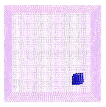
(a)

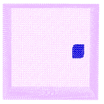
(b)

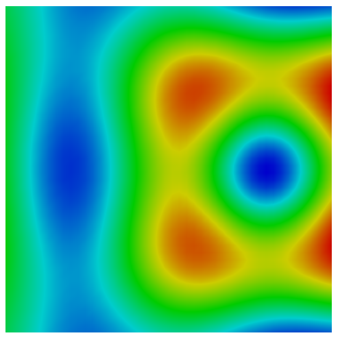
(c)

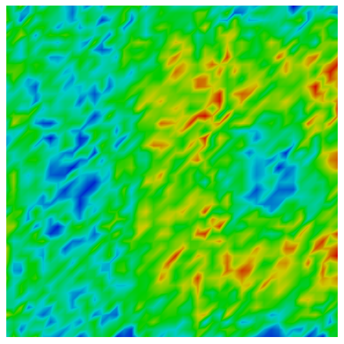
(d)

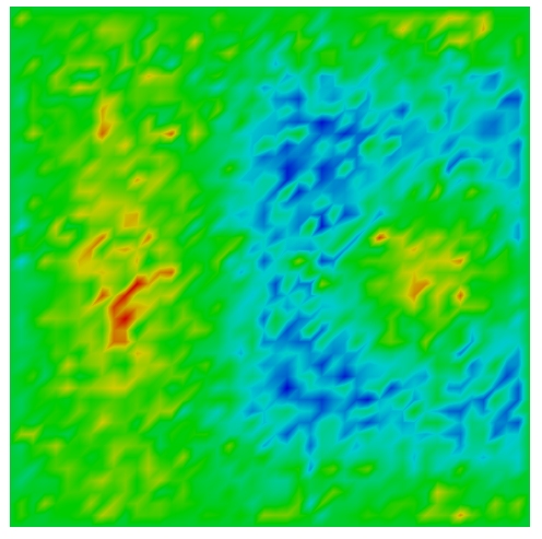
(e)

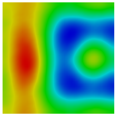
(f)

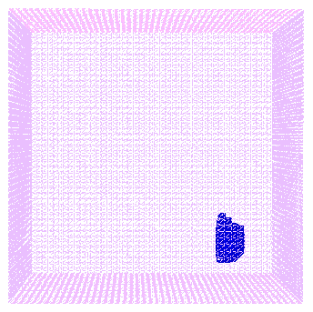
(g)

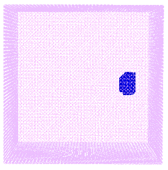
(h)

Figure 1: Case 1. $c_{comp}\left(x\right)=c_{7,2}\left(x\right),$ $\max c_{comp}\left(x\right)=2.99.$ The relative error in the maximal value is $\left(3/2.99-1\right)\cdot 100\%=0.33\%.$

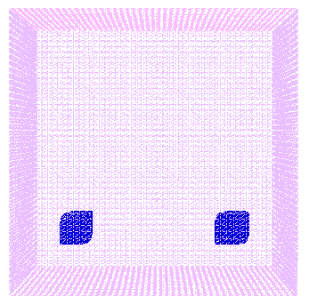
(a)

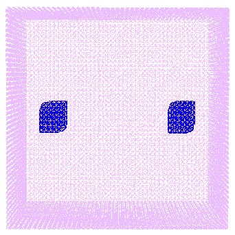
(b)

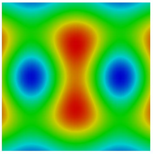
(c)

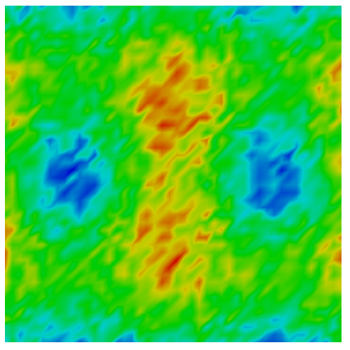
(d)

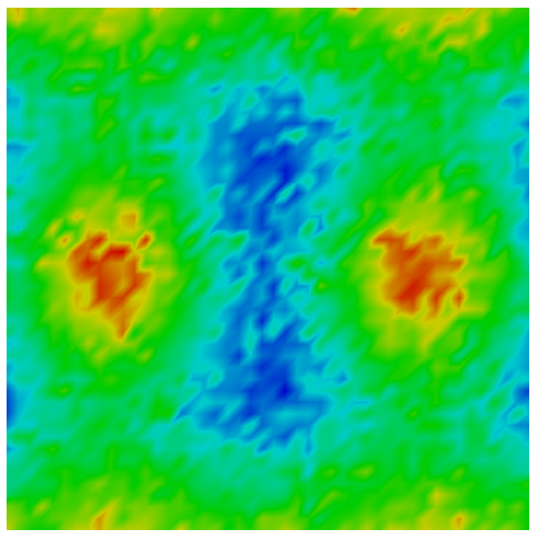
(e)

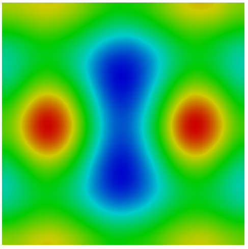
(f)

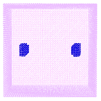
(g)

(h)

Figure 2: Case 2. $c_{comp}\left(x\right)=c_{7,2}\left(x\right),$ $\max c_{comp}\left(x\right)=3.11$. The relative error in the maximal value is $3.67\%.$.

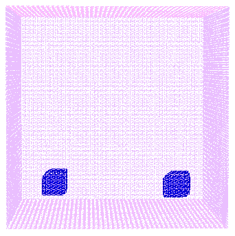
(a)

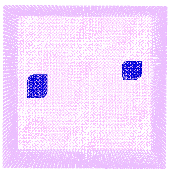
(b)

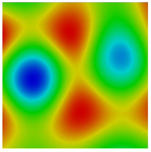
(c)

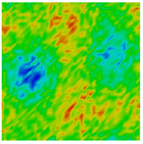
(d)

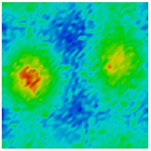
(e)

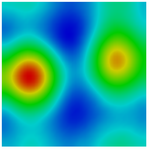
(f)

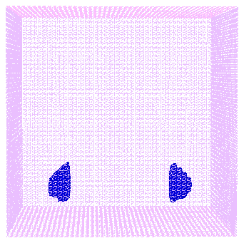
(g)

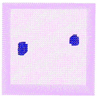
(h)

Figure 3: Case 3. $c_{comp}\left(x\right)=c_{7,2}\left(x\right),$ $\max c_{comp}\left(x\right)=3.00$. The relative error in the maximal value is $0\%.$

9 Summary

The globally convergent numerical method of the first type, which was previously developed in [2, 14, 19, 28, 29], is extended to the case of the frequency dependent data. The algorithm is developed and its global convergence is proved. Our method is numerically implemented and tested for the case of backscattering noisy data. Computational results demonstrate quite a good accuracy of this technique in imaging of locations of inclusions, maximal values of the target coefficient $c\left(x\right)$ in them and their shapes.

Acknowledgments

This work was supported by US Army Research Laboratory and US Army Research Office grant W911NF-15-1-0233 and by the Office of Naval Research grant N00014-15-1-2330.

References

- [1] G. Bao, P. Li, J. Lin and F. Triki, Inverse scattering problems with multi-frequencies, Inverse Problems, 31, 093001, 2015.
- [2] L. Beilina and M.V. Klibanov, Approximate Global Convergence and Adaptivity for Coefficient Inverse Problems, Springer, New York, 2012.
- [3] L. Beilina and M.V. Klibanov, Globally strongly convex cost functional for a coefficient inverse problem, Nonlinear Analysis: Real World Applications, 22, 272-288, 2015.
- [4] L. Beilina, Energy estimates and numerical verification of the stabilized domain decomposition finite element/finite difference approach for the Maxwell’s system in time domain, Central European Journal of Mathematics, 11, 702–733, 2013.
- [5] A.L. Bukhgeim and M.V. Klibanov, Uniqueness in the large of a class of multidimensional inverse problems, Soviet Mathematics Doklady, 17, 244-247, 1981.
- [6] D. Colton and R. Kress, Inverse Acoustic and Electromagnetic Scattering Theory, Springer, New York, 1992.
- [7] D. Gilbarg and N.S. Trudinger, Elliptic Partial Differential Equations of Second Order, Springer, New York, 1984.
- [8] F. Hecht, New development in FreeFem++, J. Numerical Mathematics, 20, 251–265, 2012.
- [9] O.Yu. Imanuvilov and M. Yamamoto, Global uniqueness and stability in determining coefficients of wave equations, Commun. in Partial Differential Equations, 26, 1409-1425, 2001.
- [10] S. I. Kabanikhin, A. D. Satybaev, and M. A. Shishlenin, Direct Methods of Solving Inverse Hyperbolic Problems, VSP, Utrecht, 2005.
- [11] S.I. Kabanikhin, K.K. Sabelfeld, N.S. Novikov and M. A. Shishlenin, Numerical solution of the multidimensional Gelfand-Levitan equation, J. Inverse and Ill-Posed Problems, 23, 439-450, 2015.
- [12] M. V. Klibanov, Inverse problems and Carleman estimates, Inverse Problems, 8, 575–596, 1992.
- [13] M.V. Klibanov, Carleman estimates for global uniqueness, stability and numerical methods for coefficient inverse problems, J. Inverse and Ill-Posed Problems, 21, 477-560, 2013.
- [14] M.V. Klibanov, M.A. Fiddy, L. Beilina, N. Pantong and J. Schenk, Picosecond scale experimental verification of a globally convergent numerical method for a coefficient inverse problem, Inverse Problems, 26, 045003, 2010.
- [15] M.V. Klibanov, Global convexity in a three-dimensional inverse acoustic problem, SIAM J. Math. Anal., 28, 1371-1388, 1997.
- [16] M.V. Klibanov and N.T. Thành, Recovering of dielectric constants of explosives via a globally strictly convex cost functional, SIAM J. Appl. Math., 75, 518-537, 2015.
- [17] M.V. Klibanov and V.G. Kamburg, Globally strictly convex cost functional for an inverse parabolic problem, Mathematical Methods in the Applied Sciences, 39, 930-940, 2016.
- [18] M.V. Klibanov and V.G. Romanov, Two reconstruction procedures for a 3-D phaseless inverse scattering problem for the generalized Helmholtz equation, Inverse Problems, 32, 015005, 2016.
- [19] A.V. Kuzhuget, L. Beilina, M.V. Klibanov, A. Sullivan, L. Nguyen and M.A. Fiddy, Blind backscattering experimental data collected in the field and an approximately globally convergent inverse algorithm, Inverse Problems, 28, 095007, 2012.
- [20] O.A. Ladyzhenskaya and N.N. Uralceva, Linear and Quasilinear Elliptic Equations, Academic Press, New York, 1969.
- [21] J. Li, H. Liu and J. Zou, Locating multiple multiscale acoustic scatterers, SIAM Multiscale Model. Simul., 12, 927–952, 2014.
- [22] J. Li, H. Liu and Q. Wang, Enhanced multilevel linear sampling methods for inverse scattering problems, J. Comput. Phys., 257, 554–571, 2014.
- [23] J. Li, H. Liu, Z. Shang and H. Sun, Two single-shot methods for locating multiple electromagnetic scattereres, SIAM J. Appl. Math., 73, 1721-1746, 2013.
- [24] R.G. Novikov, A multidimensional inverse spectral problem for the equation , Funct. Anal. Appl., 22, 263–272, 1988.
- [25] R.G. Novikov, The inverse scattering problem on a fixed energy level for the two-dimensional Schrödinger operator, J. Functional Analysis, 103, 409-463, 1992.
- [26] V.G. Romanov, Investigation Methods for Inverse Problems, VSP, Utrecht, 2002.
- [27] V.G. Romanov, Inverse problems for differential equations with memory, Eurasian J. of Mathematical and Computer Applications, 2, issue 4, 51-80, 2014.
- [28] N. T. Thành, L. Beilina, M. V. Klibanov and M. A. Fiddy, Reconstruction of the refractive index from experimental backscattering data using a globally convergent inverse method, SIAM Journal on Scientific Computing, 36, B273–B293, 2014.
- [29] N. T. Thành, L. Beilina, M. V. Klibanov and M. A. Fiddy, Imaging of buried objects from experimental backscattering time dependent measurements using a globally convergent inverse algorithm, SIAM J. Imaging Sciences, 8, 757-786, 2015.
- [30] A.N. Tikhonov, A.V. Goncharsky, V.V. Stepanov and A.G. Yagola, Numerical Methods for the Solution of Ill-Posed Problems, London: Kluwer, 1995.
- [31] R. Triggiani and Z. Zhang, Global uniqueness and stability in determining the electric potential coefficient of an inverse problem for Schrödinger equations on Riemannian manifolds, J. Inverse and Ill-Posed Problems, 23, 587-609, 2015.
- [32] B.R. Vainberg, Asymptotic Methods in Equations of Mathematical Physics, Gordon and Breach Science Publishers, New York, 1989.
- [33] M. Yamamoto, Carleman estimates for parabolic equations and applications. Topical Review. Inverse Problems, 25, 123013, 2009.